Fusing multi‑scale information
in convolution network for MR image
super‑resolution reconstruction
Chang Liu
1,2,3,4, Xi Wu
5*, Xi Yu
1,4, YuanYan Tang
6, Jian Zhang
7and JiLiu Zhou
5Background
A higher magnetic resonance image (MRI) resolution often results in fewer image artifacts, such as the partial volume effect (PVE), and a higher algorithm accuracy in the post-image processing steps (e.g., image registration and image segmentation). However, the MR resolution is affected by various physical, technological and eco-nomic limitations. Thus, increasing the spatial resolution is of considerable interest in the field of medical image processing. Conventional super-resolution (SR) methods
Abstract
Background: Magnetic resonance (MR) images are usually limited by low spatial resolution, which leads to errors in post-processing procedures. Recently, learning-based super-resolution methods, such as sparse coding and super-resolution convolu-tion neural network, have achieved promising reconstrucconvolu-tion results in scene images. However, these methods remain insufficient for recovering detailed information from low-resolution MR images due to the limited size of training dataset.
Methods: To investigate the different edge responses using different convolution kernel sizes, this study employs a multi-scale fusion convolution network (MFCN) to perform super-resolution for MRI images. Unlike traditional convolution networks that simply stack several convolution layers, the proposed network is stacked by multi-scale fusion units (MFUs). Each MFU consists of a main path and some sub-paths and finally fuses all paths within the fusion layer.
Results: We discussed our experimental network parameters setting using simulated data to achieve trade-offs between the reconstruction performance and computa-tional efficiency. We also conducted super-resolution reconstruction experiments using real datasets of MR brain images and demonstrated that the proposed MFCN has achieved a remarkable improvement in recovering detailed information from MR images and outperforms state-of-the-art methods.
Conclusions: We have proposed a multi-scale fusion convolution network based on MFUs which extracts different scales features to restore the detail information. The structure of the MFU is helpful for extracting multi-scale information and making full-use of prior knowledge from a few training samples to enhance the spatial resolution. Keywords: Super-resolution reconstruction, Multi-scale information fusion,
Convolution network, Magnetic resonance imaging
Open Access
© The Author(s) 2018. This article is distributed under the terms of the Creative Commons Attribution 4.0 International License (http://creat iveco mmons .org/licen ses/by/4.0/), which permits unrestricted use, distribution, and reproduction in any medium, provided you give appropriate credit to the original author(s) and the source, provide a link to the Creative Commons license, and indicate if changes were made. The Creative Commons Public Domain Dedication waiver (http://creat iveco mmons .org/publi cdoma in/zero/1.0/) applies to the data made available in this article, unless otherwise stated.
RESEARCH
in non-homogeneous areas and result in blurred images.
Super-resolution technologies have been implemented in the following two major categories. (1) During the acquisition stage, k-space data can be manipulated, and the parameters can be configured to improve the spatial resolution [3, 4]. (2) Dur-ing the post-processDur-ing stage, conventional image super-resolution methods can be adapted and applied to MRI. Peled and Yeshurun [5] and Greenspan [6] applied an iterative back-projection method to 2D and 3D MRI super-resolution. The resolution enhancement [7] and non-local method [8] were also implemented and extended to reconstruct a high-resolution image from corresponding low-resolution image with inter-modality priors from another HR image [9].
Recently, sparse coding (SC)-based super-resolution approaches have been shown to have good performance and accuracy in several applications, including de-nois-ing [10], and restoration [11]. Donoho [12] reconstructed MRI from a small subset of k-space samples to solve the super-resolution problem. Yang et al. [13] and Zeyed et al. [14] implemented sparse representations of natural images and successfully adapted these representations to MRI [15]. The sparse representation-based super-resolution method involves several steps. First, low-super-resolution and high-super-resolution dictionaries are trained by overlapping patches cropped from low- and high-reso-lution images, respectively. Based on this, the low-resohigh-reso-lution images are considered sparse combinations of patches in the low-resolution dictionary space. Finally, the solved sparse coefficients are mapped onto a high-resolution dictionary space and used to reconstruct the high-resolution version. Since the conventional sparse rep-resentation method trains a dictionary based on a gradient or Sobel features, the reconstructed high-resolution images are not robust and are sensitive to noise. Addi-tionally, the independent SC of the sequential patches cannot ensure the optimal reconstruction of entire dataset [16, 17].
In the literature, a few studies have addressed the MRI super-resolution problem using the deep CNN approach. A higher dimension (3D) MRI is associated with a huge com-putational burden and complicates the training more than a 2D version. In addition, a large amount of training data is not always available. To overcome these challenges, we were inspired by studies using multi-scale analyses and residual networks [15, 33]; we fused multi-scale information and propagated this information along the convolution network. Unlike conventional deep CNN learning, we observed that fusing multi-scale information in a convolution network makes it easier to achieve 3D MRI super-reso-lution using a limited amount of training data. In addition, the experiments indicated that the multi-scale fusion convolution network (MFCN) preserved detailed image information during the reconstruction procedure, which is essential for medical image applications.
The contributions of our work include the following three aspects:
• We illustrated different convolution responses using different convolution kernel sizes experimentally and demonstrated that fusing different responses was ben-eficial for recovering detailed information from a low-resolution image. Conven-tional CNNs can learn different scale information from different convolution lay-ers, but they are unable to integrate different scale information and decrease the error during the back-propagation procedure.
• To overcome the drawback of conventional CNNs and integrate multi-scale infor-mation induced by different convolution layers, we developed an MFCN. The proposed network, which is stacked by a multi-scale fusion unit (MFU), is a full convolution network that is capable of learning end-to-end mapping between low- and resolution images, makes full use of prior knowledge from high-resolution images, and uses multi-scale information to infer missed details in low-resolution images. This network exhibits an outstanding performance in MRI reconstruction. The proposed network also has a faster convergence speed than the traditional convolution network. This network is capable of learning feature maps and provides exact guidance for the design of network architecture.
• Contrary to the argument that “deeper is not better” [26], we found that a larger kernel size, an increased number of kernels, and a deeper structure are all ben-eficial for improving the reconstruction performance. However, these features increase the computational burden and converge more slowly. Considering the ideal trade-off between performance and speed, the adopted network structure has achieved a better performance with both simulated and real MRI data com-pared to some classical SR methods.
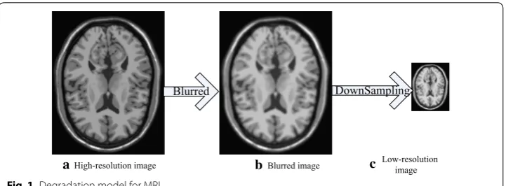
In the field of medical image analysis, a low-resolution MR image, L, can be presented as a blurred and down-sampled version of a high-resolution image, H, as follows:
where e is the noise, D is a down-sampling operator, and S is a blurring filter. The degra-dation procedure is shown in Fig. 1.
In Eq. (1), the high-resolution image can be estimated by minimizing the following cost function:
where H˜ is the reconstructed high-resolution image. However, the above problem is ill-posed, and it is difficult to find a perfect solution that satisfies Eq. (2). Normally, image patches are extracted to alleviate the ill-posed nature of the problem as follows:
where Hi and Li represent the i-th patch cropped from the high- and low-resolution
images, respectively, H˜i is the i-th reconstructed high-resolution patch and m is the number of patches. Therefore, the key issue becomes identifying the mapping relation-ship, DS, in Eq. (3) that maps the high-resolution images onto the low-resolution images.
MFCN for achieving MRI super‑resolution Analysis of the network architecture
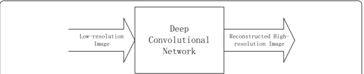
While implementing super-resolution reconstruction using deep learning, it is natural to acquire a mapping from the low- to high-resolution images. Generally, the low-reso-lution image is up-sampled to have the same size as the high-resolow-reso-lution image before SR. Previous studies [26] have successfully implemented natural image SR with convolution neural networks. The SR based on the deep convolutional network is easy to implement due to its end-to-end learning strategy. An overview of SR based on the deep convolu-tional network is shown in Fig. 2.
(1)
L=DSH+e
(2) ˜
H=arg min�DSH−L�2
(3) ˜
Hi=arg min m
i
�DSHi−Li�2
Blurred DownSampling
a b c
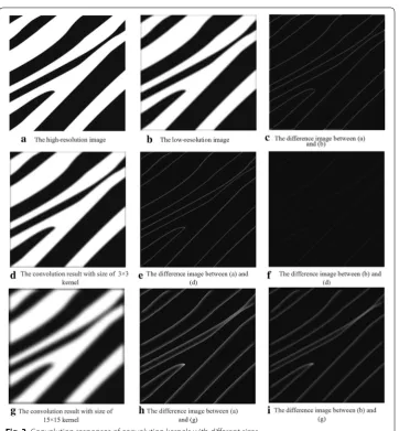
The success of convolution neural networks in SR mostly depends on the contribu-tion of the learned convolucontribu-tion kernels from the training samples. To investigate the effects of different convolution kernels in SR tasks, we generated two distinct kernels with sizes of 3×3 and 15×15 for a better visual representation. Then, the two kernels were applied to a simple low-resolution image. The convolution results and the differ-ence between the high-resolution and low-resolution images are shown in Fig. 3. As shown in the first row, the main difference between the high-resolution and low-resolu-tion images is at the edges. Therefore, the task of SR is to recover detailed informalow-resolu-tion, such as edges. Furthermore, the second and third rows in Fig. 3 show that convolution operations with different kernel sizes yield varying responses along the edges, and the strengths of the responses depend on the size of the convolution kernels. Due to the receptive field range of the convolution kernels with different sizes, the larger convolu-tion kernels induce stronger responses along the edges. Consequently, these convoluconvolu-tion responses are extracted as multi-scale information of the convolution kernels.
Design of multi‑scale network architecture
Due to the forward and back propagation mechanisms in the convolution neural net-work, we constructed a simple convolution network stacked by two convolution layers as shown in Fig. 4. Both convolution layers have only one convolution kernel. In the convolution network, the input low-resolution images are submitted to the network and convoluted using the following convolution layers sequentially to obtain the feature maps. This procedure is called forward propagation. After the final convolution layer, the errors in the feature maps and high-resolution images, and the difference images, are computed based on the Euclidean distance of the loss layer. The difference images are very important for adjusting the kernel parameters of the final convolution layer. All parameters of each layer are adjusted using stochastic gradient descent.
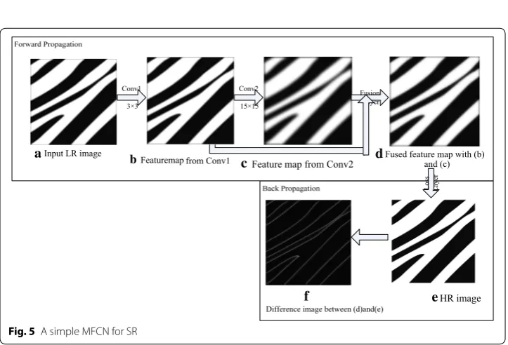
Due to the multi-scale properties of different kernel sizes, fusing different scale con-volution responses is assumed to accelerate the SR procedure. In the following study, we developed a simple MFCN as shown in Fig. 5. As depicted in Fig. 4, the MFCN has two convolution layers, and each layer has only one convolution kernel. We added a fusion layer to the network shown in Fig. 5. The function of the fusion layer is simply to add feature maps from (b) and (c). Initially, the fusion image had more details than the feature map in (c). Moreover, compared with the difference image I in Fig. 4, the difference image (f) in Fig. 5 is darker, which indicates less error between the recovered image and high-resolution image and is beneficial for accelerating the convergence in the training phase.
Therefore, it is desirable to design a convolution network that combines differ-ent scale information. Reconstructed images benefit from end-to-end learning of low/
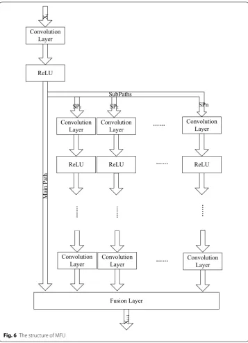
high-resolution images and multi-scale information propagation through the whole net-work structure. Inspired by residual netnet-works [33], we defined the following structure, i.e., the MFU, to fuse different convolution paths as shown in Fig. 6:
where f represents the convolution layer and ReLU. SPj(xi,W¯i) denotes the j-th sub-path in which input xi is convoluted by some convolution kernels. J is the number of
sub-paths. According to the main path and several sub-paths, different scale informa-tion is extracted by various convoluinforma-tion kernels, and then, the multi-scale informainforma-tion is combined in the fusion layer based on additional operations. Output xi+1 retains more
detailed information than the output from the traditional convolution network that is simply stacked by a convolution layer and helps accelerate the convergence. " Experi-ments" section provides a validation.
(4) xi+1=f(xi,W0)+
J
j=1
SPj(xi,W¯i)
Based on the above-mentioned MFU, we developed the MFCN shown in Fig. 7. This network is stacked by a few MFUs and a reconstruction layer, in which the reconstruc-tion layer is a convolureconstruc-tion layer with one kernel.
Conv1
3×3
Conv2
15×15
Loss Laye
r
a b c
d e
Input LR image Feature map from Conv1 Feature map from Conv2
Difference image between (c)and(d)
based on Euclidean distance HR image
Fig. 4 A simple convolution network for SR
Conv1
3×3
Conv2
15×15
Fusion Layer
Loss Layer
a b
c d
e f
Input LR image
Featuremap from Conv1 Feature map from Conv2 Fused feature map with (b) and (c)
Difference image between (d)and(e) HR image
Experiments
To evaluate the reconstruction performance of the proposed MFCN for structural MR images, we designed an extensive set of validation experiments using both simulated and real MR images. Furthermore, several methods were employed for comparison, includ-ing bicubic interpolation, non-local mean (NLM) [11], sparse coding [13], and super-resolution convolution neural network (SRCNN) [26].
Convolution Layer
ReLU
Main Path
SP1
Convolution Layer
ReLU
Convolution Layer
ReLU SP2
Convolution
Layer Convolution Layer
Fusion Layer
Convolution Layer
ReLU
Xi+
1
SubPaths
SPn
Convolution Layer
Experimental settings
The proposed MFCN was run on an Ubuntu 14.04 with an Intel Xeon E5-2620 processor at 2.4 GHz, K80 GPU and the 96 GB of RAM based on the Caffe deep learning frame-work [34].
Brain MR image sets
In this paper, the proposed MFCN was tested using different MR image sets, including both simulated and real images.
• Simulated MR images were generated using an MRI simulator and obtained from the BrainWeb brain database [35]. The simulation provides volumes acquired in the axial plane with dimensions of 181×217×181 pixels and 1 mm3 resolution.
• Real T1-weighted brain MR images were obtained from thirty subjects and were acquired using a GE MR750 3.0T scanner with two different spatial resolutions of 1 mm×1 mm×1 mm and 3 mm×3 mm×3 mm . For the high-resolution MR images, each anatomical scan had 156 axial slices with a size of 256×256 pixels. The low-resolution MR images only included 52 axial slices.
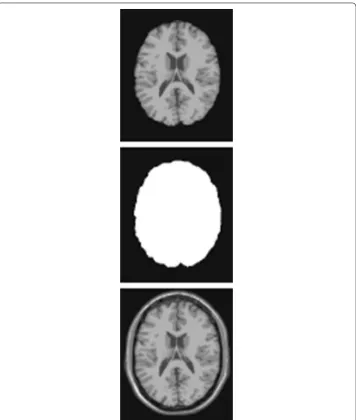
Similarly to the pre-processing step in [15], the skull and skin were removed from the MR images using a brain extraction tool (BET) [36] to eliminate the influence of the background. The resulting MR image is shown in Fig. 8. For the training set, high-res-olution patches were extracted from each slice of a brain region with a size of 33×33
pixels. To obtain low-resolution patches, a blurring and down-sampling operation was applied to the extracted brain regions. Then, a bi-cubic interpolator was implemented. Finally, low-resolution image patches were acquired from the interpolated brain region.
For the learning-based method, we constructed the same training set to ensure con-sistency. The sparsity regularization parameter was set to 0.01 for the sparse coding-based reconstruction as reported in the literature [15]. The learning rate was set to 0.001. The network was trained using mini-batches of size 32.
Quantitative performance measures
To quantitatively evaluate the performance of the reconstruction of different MR image sets, three different metrics were used to compare the original high-resolution images (x) with the reconstructed images (y).
• The signal-to-noise ratio (SNR) was used to compare the level of the recon-structed image with the level of the background noise:
Input LR
Image MFU MFU Reconstruction Layer Output HR Image
where xk and yk are the image intensities at position k.
• The peak SNR (PSNR) was used to measure the reconstruction accuracy between the reconstructed image and the original image:
(5) SNR(x,y)=10 log10
k|xk|2
k xk−yk
2
(6)
PSNR(x,y)=10 log10
R
�
1
|�| �
k∈� � �xk−yk
� �
2
where is the brain region, and R is the maximum pixel value in the low-resolution
image.
• The structural similarity index (SSIM) [37] was used to measure the similarity between the two images, which is more consistent with human visual systems and perception.
where c1=(k1L)2 , c2=(k2L)2 , and L are the dynamic range, k1=0.01 , and k2=0.03 . The terms µx and µy are the mean values of images x and y, respectively; σx and σy are the standard noise variance in images x and y, respectively; and σxy is the covariance of x and y.
Network architecture analysis
To achieve deep learning, a large number of parameters must be tuned, which affected the reconstruction performance of the proposed network. In this section, we discuss these various factors and investigate the best trade-off between performance and speed in the simulated data. For the simulated data, the training set was con-structed from the BrainWeb database using 30 real MR brain slices acquired by sam-pling 600 random image locations from each slice, and the test data were obtained from the slices excluded from the training set. For a baseline, the parameter configu-ration is listed in Tables 1, 2 and 3, where nMFU is the number of multi-scale fusion units, MFUn is the n-th multi-scale fusion units, sk is the size of convolution kernel,
nk is the number of convolution kernel, nSubPath is the number of sub-paths in each
MFU, and nLayer is the number of convolution layers in each sub-path.
(7) SSIM(x,y)= (2µxµy+c1)(2σxy+c2)
(µ2x+µ2y+c1)(σx2+σy2+c2)
Table 1 The network configurations of the baseline in MFCN
Network nMFU sk/nk in reconstruction layer
MFCNBL 2 5/1
Table 2 The MFU1 configurations in MFCNBL
sk/nk of main path in MFU nSubPath nLayer in each sub‑path sk/nk of in sub‑path
9/32 1 1 1/32
Table 3 The MFU2 configurations in MFCNBL
sk/nk of main path in MFU nSubPath nLayer in each sub‑path sk/nk of in sub‑path
Parameter discussion for main path
In this section, we develop several networks that have the same structure as MFCNBL , except for a different kernel size and number in the main path in the MFU, and a final reconstruction layer to examine the reconstruction performance.
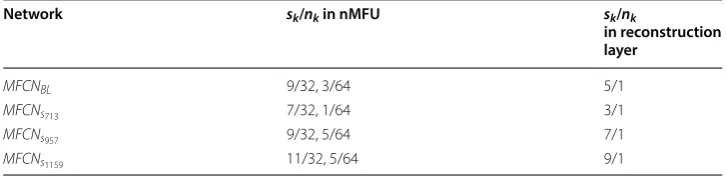
Kernel size Several image recognition and recognition experiments have demonstrated that if the number of kernels in each layer increases, the performance will improve. However, increasing the number of kernels also requires more time to train the network. Therefore, we compared the influence of the different kernel sizes on the reconstruction performance. The detailed parameter configuration is shown in Table 4.
The average PSNR with an upscaling factor of 3 is shown in Fig. 9. The proposed network with different kernel sizes always achieved a better performance than the bi-cubic interpolation and SC. Furthermore, the MFCNBL and MFCNs957 networks had a comparable PSNR, while the MFCNs713 network had a worse performance. One possible reason is that the MFCNs713 network had limited descriptive power for the super-resolution reconstruction due to the fewer parameters. However, we also observed that although the PSNR of the MFCNs1159 network increases as the
itera-tion number increases, it always performs worse than the MFCNBL and MFCNs957 networks within limited iterative numbers, which probably illustrated that the
layer
MFCNBL 9/32, 3/64 5/1
MFCNs713 7/32, 1/64 3/1
MFCNs957 9/32, 5/64 7/1
MFCNs1159 11/32, 5/64 9/1
0 2 4 6 8 10
x 104 35.5
36 36.5 37 37.5 38 38.5 39 39.5 40 40.5
Epoch
Average PSNR(dB)
Bicubic Sparse Coding MFCNs
713
MFCNs
BL
MFCNs
957
MFCNs
1159
networks with bigger kernel size need more training time to converge to achieve a better reconstruction performance, as shown in Table 5. Consequently, increasing the kernel size properly was helpful for achieving superior performance, but consid-ering the balance between the reconstruction performance and the computational efficiency, bigger kernel size is not always good.
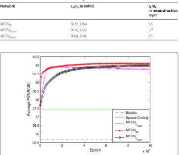
Kernel numbers Generally, increasing the kernel number will improve perfor-mance. Based on the baseline network with 32 and 64 kernel numbers in the main path in MFU, we increased the kernel number to 64 and 96 and maintained the ker-nel number in the last reconstruction layer 1, called MFCNn64961 . We also
investi-gated fewer kernel numbers in the main path in MFCN with 16 and 32, referred to as
MFCNn16321 . The detailed configuration is shown in Table 6.
Table 5 The average SNR, PSNR, SSIM and reconstruction time of each slice with a different kernel size in the main path in MFU and the final reconstruction layer at the 105 iteration
Network SNR PSNR SSIM Time (s)
MFCNs713 26.574 39.6064 0.9875 0.009123
MFCNBL 27.0741 40.1064 0.9891 0.019142
MFCNs957 27.0415 40.0738 0.989 0.020472
MFCNs1159 26.9858 40.0181 0.9885 0.027577
Table 6 The different kernel number configurations
Network sk/nk in nMFU sk/nk
in reconstruction layer
MFCNBL 9/32, 3/64 5/1
MFCNn16321 9/16, 3/32 5/1
MFCNn64961 9/64, 3/96 5/1
0 2 4 6 8 10
x 104 35.5
36 36.5 37 37.5 38 38.5 39 39.5 40 40.5
Epoch
Average PSNR(dB) Bicubic
Sparse Coding MFCNn
16321
MFCNBL MFCNn
64961
These results are shown in Fig. 10. The MFCNn16321 network had the worst
per-formance. In the initial iteration, the MFCNn64961 network had a worse performance
than the baseline MFCNBL network. The performance of the MFCNn64961 network
improved as the iteration number increased. It is possible to surpass the base-line network with additional training time likely because the MFCNn64961 network
requires more learning of the network parameters. This network fails to converge during the 105 epochs; therefore, it is not superior to MFCN
BL with 32 and 64 kernel numbers.
Sub‑path parameter discussion
In this section, we discuss the influence of the sub-paths (e.g., the kernel size and the number of convolution layers in each sub-path) and the effects of preserving an ReLU layer before its addition to the MFU.
Kernel size of convolutional layers in the sub‑paths
First, we discuss the kernel size of the convolution layers. As shown in Table 7, we attempted to enlarge the kernel size from 1×1 in the baseline network to 3×3 in the
convolution layers in the sub-path ( MFCNS3 ). The result is shown in Fig. 11. A superior performance was achieved in MFCNS3 . As discussed in "Sub-path parameter discussion" section, the same conclusion was reached, i.e., a wider kernel size is helpful for improv-ing performance.
within MFU
MFCNBL 1/32, 1/64
MFCNS3 3/32, 3/64
0 2 4 6 8 10
x 104 35.5
36 36.5 37 37.5 38 38.5 39 39.5 40 40.5
Epoch
Average PSNR(dB) Bicubic
Sparse Coding MFCNBL MFCNS
3
Number of convolution layers in the sub‑paths
In the MFCNBL , the sub-path in each MFU contains a convolution layer. Increasing the number of convolution layers in the sub-path is helpful for adding depth to the network. Therefore, we further examined networks with more convolution layers and set two convolution layers in the sub-path of each unit. The detailed configuration is shown in Table 8. Although the average PSNR shown in Fig. 12 demonstrated that the baseline network with one convolution layer ( MFCNBL ) was superior to the network with two convolution layers ( MFCNL2 ), the performance of MFCNL2 approached that of MFCNBL
near the 105 iteration and could potentially surpass the baseline networks with higher
iterative numbers. MFCNL2 may need to learn more parameters and converges more
slowly than MFCNBL . Consequently, a balance between the reconstruction performance and convergence speed is needed.
ReLU before the fusion layer
Previous studies [33] have shown that the “residual” unit should be in the range of
(−∞,+∞) and suggested removing the ReLU before the addition of the fusion layer to
achieve a lower error in the image classification. To confirm the performance of ReLU in MFU for MRI super-resolution reconstruction, we also investigated a network structure by adding ReLU before the addition of each MFU. The other settings remained the same as those in the baseline network ( MFCNBL ). As shown in Fig. 13, removing ReLU before add-ing the fusion layer exceeded the performance compared to when ReLU was maintained. Table 8 The different kernel number configurations
Network nLayer in each sub‑path
sk/nk of sub‑path within MFU1
sk/nk of sub‑path within MFU2
MFCNBL 1 1/32 1/64
MFCNL2 2 1/32, 1/32 1/64, 1/64
0 2 4 6 8 10
x 104 35.5
36 36.5 37 37.5 38 38.5 39 39.5 40 40.5
Epoch
Average PSNR(dB) Bicubic
Sparse Coding MFCNBL MFCNL
2
0 1 2 3 4 5 6 7 8 9 10 x 104 35.5
36 36.5 37 37.5 38 38.5 39 39.5
Epoch
Average PSNR(dB
)
Bicubic Sparse Coding Remove Relu Keep Relu
Fig. 13 Comparison of MFU with and without ReLU before adding the fusion layer
0 2 4 6 8 10
x 104 35.5
36 36.5 37 37.5 38 38.5 39 39.5 40 40.5
Epoch
Average PSNR(dB)
Bicubic Sparse Coding MFCNU
1
MFCN BL MFCNU
3
Fig. 14 The average PSNR with different numbers of MFUs
Table 9 The different MFUs configurations Network sk/nk of sub‑path
within MFU1
sk/nk of sub‑path within MFU2
sk/nk of sub‑path within MFU3
MFCNBL 1/32 1/64 N/A
MFCUU1 1/32 N/A N/A
MFCUU3 1/32 1/32 1/64
Number of MFUs
improved performance. In addition to increasing the number of convolution lay-ers in the sub-path in "Sub-path parameter discussion", we attempted to deepen the network by adding several MFUs. The detailed configuration is shown in Table 9. As shown in Fig. 14, a network with one MFU ( MFCUU1 ) had a worse performance than
the baseline network with two MFUs ( MFCNBL ). Initially, the networks with three
MFUs ( MFCUU3 ) were superior to the baseline network, but their performance
wors-ened after approximately 20K iterations, and the curve increased by nearly 105 iter-ative numbers. Therefore, it is difficult to achieve the same conclusion as [26]. We believe that this trend does not oppose the advantage of the network depth. Deeper
work from 2×10 to 10 iterations.
Learned feature maps
To investigate why the proposed network is capable of super-resolution reconstruc-tions, some feature maps were studied using different layers and are shown in Fig. 15. As shown in Fig. 15, different kernels in the main path extract distinct information from low-resolution images, such as different directions, as shown in the second row. Convolution layers in the sub-path recover different modalities based on the feature maps in the second row as shown in the third row. The feature maps in the second and third rows are complementary, and the final fusion layer with the addition opera-tion in MFU is helpful for combining the complementary informaopera-tion as shown in the fourth row. For a better understanding of MFU, we further compared MFCNBL
and the traditional convolution network (SRCNN) using the same configurations. The results are shown in Fig. 16. The MFCN was always superior to the SRCNN.
In summary, we investigated the parameter settings of the proposed network and decomposed MFU to visualize the feature maps of the main path and sub-path. Each of these experiments indicated that a larger kernel size, an increased kernel num-ber in the convolution layers, and a deeper network are helpful for improving the reconstruction performance. However, many parameters need to be learned, and the convergence is, therefore, slow. Consequently, we must compromise between perfor-mance and efficiency.
Comparisons to state‑of‑the‑art approaches
In previous experiments, the influence of different parameters on networks and reconstruction performance has been discussed. To balance the performance and
0 2 4 6 8 10
x 104 36
36.5 37 37.5 38 38.5 39 39.5 40 40.5
Epoch
Average PSNR(dB)
SRCNN MFCNBL
computational efficiency, we adopted the above-mentioned baseline network due to its good performance-speed trade-off. Once the network architecture was fixed, the super-resolution reconstruction experiments were carried out to validate the performance of the proposed method. In this section, quantitative and qualitative results of the pro-posed method were compared with results of certain classical methods for different up-sampling factors f, including f= 2, 3 and 4. The implementation of existing methods was achieved using publicly available codes provided by the authors. For the MFCN and SRCNN, we trained the network using 105 iterations.
Different up‑sampling factors
As shown in Table 10, the proposed method always yielded the best scores with different evaluation metrics. Figure 17 also illustrates the reconstructed MR images using differ-ent methods in a single slice. Notably, within the red circle of Fig. 17, it can be found that the reconstructions based on MFCN were able to restore more detailed information for the MR images than those based on the other classical methods.
Table 10 Quantitative evaluation (RMSE, SNR, PSNR, and SSIM) of different up‑sampling factors using BrainWeb MR images
Eval. met Scale Bicubic NLM Sparse coding SRCNN MFCN
RMSE 2 2.5077 2.1112 1.7747 1.4836 1.2026 3 4.2038 3.7707 3.4262 2.8937 2.5415 4 5.849 5.5588 5.0577 4.6946 4.5196 SNR 2 27.1376 28.636 30.1495 31.7244 33.5375 3 22.6394 23.5894 24.422 25.9595 27.0741 4 19.767 20.2123 21.0326 21.7213 22.0571 PSNR 2 40.1699 41.6684 43.1819 44.7567 46.5698 3 35.6717 36.6218 37.4262 38.9918 40.1064 4 32.7993 33.2446 34.056 34.7536 35.0895 SSIM 2 0.9891 0.9923 0.9945 0.9963 0.9975 3 0.9678 0.9743 0.9788 0.9864 0.9891 4 0.9375 0.9434 0.9529 0.9639 0.9662
Ground Truth Bicubic NLM Sparse Coding SRCNN MFCN
PSNR=34.89 PSNR=35.88 PSNR=36.85 PSNR=37.08 PSNR=38.18
Evaluation of real data
We further examined the performance of the MFCN using a real dataset. We selected fifteen subjects as the training data and the remaining subjects as the test data. Fig-ure 18 shows representative image reconstruction results using various methods. From left to right, the first row shows the high-resolution image, the corresponding low-resolution image, and the results of NLM, sparse coding, SRCNN, and MFCN. The close-up views of the selected regions are also shown for better visualization. The results of NLM show severe blurring artifacts, and the results of sparse coding are better than those of NLM. The contrast is enhanced in the SRCNN results, while the proposed MFCN is the best for preserving edges and achieving the highest PSNR value as shown in Fig. 18. The quantitative results using the real datasets are illus-trated in Fig. 19. As shown in Fig. 19, the total distribution of PSNRs for MFCN are better than others; The mean (small square in the box) and the median (the horizontal
PSNR=35.08 PSNR=35.85 PSNR=35.8 PSNR=36.56 Fig. 18 Visual comparison of the different methods using real data
NLM Sparse Coding SRCNN MFCN
32 34 36 38 40 42 44 46 48 50 52
Rang
e
NLM
Sparse Coding SRCNN MFCN
line in the box) of PSNR for MFCN are also greater than other one. Therefore, the proposed method significantly outperformed all compared methods.
Discussion
It is well known that the convolution neural network has a large number of network parameters and is needed for training with a large dataset to avoid over-fitting. However, due to limited MRI training data, it is difficult to achieve superior reconstruction using a standard convolution network. In this work, we developed an MFCN for MRI super-resolution reconstruction and achieving end-to-end (one-to-one) mapping between low and high-resolution images. Instead of a traditional convolution network, the network is stacked by MFUs. Each MFU consists of a main path and several sub-paths, and all paths are finally added to the fusion layer to fuse multi-scale information. We conducted several experiments and demonstrated that when the training data are limited, the pro-posed network always achieves superior reconstruction results using both simulated and real data compared with traditional SR methods, such as bi-cubic, NLM, sparse coding, and SRCNN.
An additional concern is the slow convergence speed caused by the traditional con-volution network structure. Regarding fusing multi-scale information from the main path and sub-paths in MFU, we found that the proposed network achieves faster conver-gence speed than the traditional convolution network SRCNN. As shown in Fig. 16, with the same parameter settings, the proposed network converges after 3000 epochs while SRCNN converges after 5000 epochs. Furthermore, the proposed network achieves a higher PSNR value in the same epoch. Moreover, the proposed network can recover more detailed information and has better visual effects as shown in Figs. 17 and 18.
Finally, currently used convolution networks for image super-resolution usually extract detailed information on a single scale, and the back propagation process fails to utilize prior knowledge of the high-resolution images.
According to previous research on SR [38], the extraction of multi-scale informa-tion improves the reconstrucinforma-tion results. Using the proposed convoluinforma-tion network, we also experimentally validated that differently sized convolution kernels can acquire multi-scale information as shown in Fig. 3. We found that multi-scale information can be merged and transmitted from one MFU to the next as shown in Fig. 15. Thus, the proposed network can recover detailed information and achieve better reconstruction performance.
to learn end-to-end mapping from low/high-resolution images. Simultaneously, due to the fusion of different paths in MFU, the network can extract multi-scale information to recover detailed information and accelerate the convergence speed. The extensive experiments using simulated and real data have also demonstrated that this approach is superior to other traditional methods. In addition, the proposed network architecture and experimental framework can be applied to other medical super-resolution recon-structions, such as in CT and diffusion-weighted MR imaging.
Authors’ contributions
CL conceived and designed this study and is responsible for the manuscript, XW participated in the analysis of the MRI dataset, XY, YT, JZ and JZ participated in the conception and design of this work and helped to draft the manuscript. All authors read and approved the final manuscript.
Author details
1 Department of Information Technology and Engineering, Chengdu University, Chengdu 610106, China. 2 The Clinical Hospital of Chengdu Brain Science Institute, MOE Key Lab for Neuroinformation, Center for Information in Medicine, University of Electronic Science and Technology of China, Chengdu 610054, China. 3 School of Life Science and Technol-ogy, University of Electronic Science and Technology of China, Chengdu 610054, China. 4 Key Laboratory of Pattern Rec-ognition and Intelligent Information Processing in Sichuan, Chengdu 610106, China. 5 Department of Computer Science, Chengdu University of Information Technology, Chengdu 610225, China. 6 Faculty of Science and Technology, University of Macau, Macau, China. 7 School of Physics and Electronic Engineering, Sichuan Normal University, Chengdu, China.
Acknowledgements
The authors would like to thank all participants for the valuable discussions regarding the content of this article.
Competing interests
The authors declare that they have no competing interests.
Availability of data and materials
The datasets analyzed in this study are available from the corresponding author on reasonable request.
Consent for publication
Each participant agreed that the acquired data can be further scientifically used and evaluated. For publication, we made sure that no individual can be identified.
Ethics approval and consent to participate
Written informed consent was obtained from the patient for the publication of this report and any accompanying images.
Funding
This work is supported by the National Natural Science Funds of China (Grant No. 61502059), the China Postdoctoral Science Foundation (Grant No. 2016M592656), Sichuan Science and Technology Program (Grant No. 2018JY0272), the Educational Commission of Sichuan Province of China (Grant No. 15ZA360).
Publisher’s Note
Springer Nature remains neutral with regard to jurisdictional claims in published maps and institutional affiliations.
Received: 5 May 2018 Accepted: 17 August 2018
References
1. Thévenaz P, Blu T, Unser M. Interpolation revisited medical images application. IEEE Trans Med Imag. 2000;19(7):739–58.
2. Lehmann TM, Gönner C, Spitzer K. Survey: interpolation methods in medical image processing. IEEE Trans Med Imag. 1999;18(11):1049–75.
3. Shilling RZ, Robbie TQ, Bailloeul T, Mewes K, Mersereau RM, Brummer ME. A super-resolution framework for 3-d high-resolution and high-contrast imaging using 2-d multislice MRI. IEEE Trans Med Imag. 2009;28(5):633–44. 4. Herment A, Roullot E, Bloch I, Jolivet O, De Cesare A, Frouin F, Bittoun J, Mousseaux E. Local reconstruction of
sten-osed sections of artery using multiple MRA acquisitions. Magn Reson Med. 2003;49(4):731–42.
5. Peled S, Yeshurun Y. Superresolution in MRI: application to human white matter fiber tract visualization by diffusion tensor imaging. Magn Reson Med. 2001;45(1):29–35.
7. Carmi E, Liu S, Alon N, Fiat A, Fiat D. Resolution enhancement in MRI. Magn Reson Imag. 2006;24(2):133–54. 8. Manjón JV, Coupé P, Buades A, Fonov V, Collins DL, Robles M. Non-local mri upsampling. Med Image Anal.
2010;14(6):784–92.
9. Rousseau F, Initiative ADN. A non-local approach for image super-resolution using intermodality priors. Med Image Anal. 2010;14(4):594–605.
10. Elad M, Aharon M. Image denoising via sparse and redundant representations over learned dictionaries. IEEE Trans Med Imag. 2006;15(12):3736–45.
11. Mairal J, Elad M, Sapiro G. Sparse representation for color image restoration. IEEE Trans Image Process. 2008;17(1):53–69.
12. Donoho DL. Compressed sensing. IEEE Trans Inform Theory. 2006;52(4):1289–306.
13. Yang J, Wright J, Huang TS, Ma Y. Image super-resolution via sparse representation. IEEE Trans Image Process. 2010;19(11):2861–73.
14. Zeyde R, Elad M, Protter M. On single image scale-up using sparse-representations. In: International conference on curves and surfaces. Berlin: Springer; 2010. p. 711–30.
15. Rueda A, Malpica N, Romero E. Single-image super-resolution of brain mr images using overcomplete dictionaries. Med Image Anal. 2013;17(1):113–32.
16. Wohlberg B. Efficient convolutional sparse coding. In: IEEE international conference on acoustics, speech and signal processing (ICASSP). New Jersey: IEEE; 2014 , p. 7173–77.
17. Bristow H, Eriksson A, Lucey S. Fast convolutional sparse coding. In: IEEE conference on computer vision and pattern recognition (CVPR). New Jersey: IEEE; 2013. p. 391–8.
18. Osendorfer C, Soyer H, van der Smagt P. Image super-resolution with fast approximate convolutional sparse coding. In: Neural information processing. Berlin: Springer; 2014. p. 250–7.
19. Krizhevsky A, Sutskever I, Hinton GE. Imagenet classification with deep convolutional neural networks. In: Advances in neural information processing systems; 2012. p. 1097–1105.
20. LeCun Y, Bengio Y, Hinton G. Deep learning. Nature. 2015;521(7553):436–44.
21. Cui Z, Chang H, Shan S, Zhong B, Chen X. Deep network cascade for image super-resolution. In: Computer vision– ECCV 2014. Berlin: Springer; 2014. p. 49–64.
22. Wang Z, Liu D, Yang J, Han W, Huang T. Deeply improved sparse coding for image super-resolution. arXiv preprint arXiv :1507.08905 . 2015.
23. Ji S, Xu W, Yang M, Yu K. 3d convolutional neural networks for human action recognition. IEEE Trans Patt Anal Mach Intell. 2013;35(1):221–31.
24. Bengio Y. Learning deep architectures for ai. Foundations and trends®in. Mach Learn. 2009;2(1):1–127.
25. Hinton GE, Osindero S, Teh Y-W. A fast learning algorithm for deep belief nets. Neural comput. 2006;18(7):1527–54. 26. Dong C, Loy CC, He K, Tang X. Image super-resolution using deep convolutional networks. In: IEEE transactions on
pattern analysis and machine intelligence; 2015.
27. Kim J, Lee JK, Lee KM. Accurate image super-resolution using very deep convolutional networks. arXiv preprint arXiv :1511.04587 . 2015.
28. LeCun Y, Jackel L, Bottou L, Brunot A, Cortes C, Denker J, Drucker H, Guyon I, Muller U, Sackinger E. Comparison of learning algorithms for handwritten digit recognition. In: International conference on artificial neural networks; 1995. p. 53–60.
29. LeCun Y, Jackel L, Bottou L, Cortes C, Denker JS, Drucker H, Guyon I, Muller U, Sackinger E, Simard P. Learning algo-rithms for classification: a comparison on handwritten digit recognition. Neural Netw. 1995;261:276.
30. Simonyan K, Zisserman A. Very deep convolutional networks for large-scale image recognition. arXiv preprint arXiv :1409.1556. 2014.
31. Girshick R, Donahue J, Darrell T, Malik J. Rich feature hierarchies for accurate object detection and semantic segmen-tation. In: Proceedings of the IEEE conference on computer vision and pattern recognition; 2014. p. 580–7. 32. Taigman Y, Yang M, Ranzato M, Wolf L. Deepface: closing the gap to human-level performance in face verification. In:
Proceedings of the IEEE conference on computer vision and pattern recognition; 2014. p. 1701–8.
33. He K, Zhang X, Ren S, Sun J. Identity mappings in deep residual networks. arXiv preprint arXiv :1603.05027 . 2016. 34. Jia Y, Shelhamer E, Donahue J, Karayev S, Long J, Girshick R, Guadarrama S, Darrell T. Caffe: convolutional architecture
for fast feature embedding. In: Proceedings of the ACM international conference on multimedia. New York: ACM; 2014. p. 675–8.
35. Cocosco CA, Kollokian V, Kwan RKS, Pike GB, Evans AC. Brainweb: online interface to a 3d MRI simulated brain data-base. In: NeuroImage. Kyoto: Citeseer; 1997.
36. Smith SM. Fast robust automated brain extraction. Hum Brain Map. 2002;17(3):143–55.
37. Wang Z, Bovik AC, Sheikh HR, Simoncelli EP. Image quality assessment: from error visibility to structural similarity. IEEE Trans Image Process. 2004;13(4):600–12.