An efﬁcient method to generate a perturbed parameter ensemble of a fully coupled AOGCM without ﬂux-adjustment

(1)

Geosci. Model Dev., 6, 1447–1462, 2013 www.geosci-model-dev.net/6/1447/2013/ doi:10.5194/gmd-6-1447-2013

EGU Journal Logos (RGB)

Advances in

Geosciences

Open Access

Natural Hazards

and Earth System

Sciences

Open Access

Annales

Geophysicae

Open Access

Nonlinear Processes

in Geophysics

Open Access

Atmospheric

Chemistry

and Physics

Open Access

Atmospheric

Chemistry

and Physics

Open Access

Discussions

Atmospheric

Measurement

Techniques

Open Access

Atmospheric

Measurement

Techniques

Open Access

Discussions

Biogeosciences

Open Access Open Access

Biogeosciences

Discussions

Climate

of the Past

Climate

of the Past

Discussions

Earth System

Dynamics

Earth System

Dynamics

Discussions

Geoscientific

Instrumentation

Methods and

Data Systems

Open Access

_{Geoscientific}

Instrumentation

Methods and

Data Systems

Open Access

Discussions

Geoscientific

Model Development

Geoscientific

Model Development

Discussions

Hydrology and

Earth System

Sciences

Open Access

Hydrology and

Earth System

Sciences

Open Access

Discussions

Ocean Science

Discussions

Solid Earth

Discussions

The Cryosphere

Discussions

Natural Hazards

and Earth System

Sciences

Open Access

Discussions

An efficient method to generate a perturbed parameter ensemble of

a fully coupled AOGCM without flux-adjustment

P. J. Irvine1, L. J. Gregoire2, D. J. Lunt2, and P. J. Valdes2

1_{Institute for Advanced Sustainability Studies IASS, Potsdam, Germany} 2_{School of Geographical Sciences, University of Bristol, UK}

Correspondence to: P. J. Irvine ([email protected])

Received: 9 January 2013 – Published in Geosci. Model Dev. Discuss.: 6 February 2013 Revised: 10 July 2013 – Accepted: 29 July 2013 – Published: 10 September 2013

Abstract. We present a simple method to generate a perturbed parameter ensemble (PPE) of a fully-coupled atmosphere-ocean general circulation model (AOGCM), HadCM3, without requiring flux-adjustment. The aim was to produce an ensemble that samples parametric uncertainty in some key variables and gives a plausible representation of the climate. Six atmospheric parameters, a sea-ice parame-ter and an ocean parameparame-ter were jointly perturbed within a reasonable range to generate an initial group of 200 mem-bers. To screen out implausible ensemble members, 20 yr pre-industrial control simulations were run and members whose temperature responses to the parameter perturbations were projected to be outside the range of 13.6±2◦_{C, i.e.}

near to the observed pre-industrial global mean, were dis-carded. Twenty-one members, including the standard unper-turbed model, were accepted, covering almost the entire span of the eight parameters, challenging the argument that with-out flux-adjustment parameter ranges would be unduly re-stricted. This ensemble was used in 2 experiments; an 800 yr pre-industrial and a 150 yr quadrupled CO2simulation. The

behaviour of the PPE for the pre-industrial control compared well to ERA-40 reanalysis data and the CMIP3 ensemble for a number of surface and atmospheric column variables with the exception of a few members in the Tropics. How-ever, we find that members of the PPE with low values of the entrainment rate coefficient show very large increases in upper tropospheric and stratospheric water vapour concentra-tions in response to elevated CO2and one member showed

an implausible nonlinear climate response, and as such will be excluded from future experiments with this ensemble. The outcome of this study is a PPE of a fully-coupled AOGCM

which samples parametric uncertainty and a simple method-ology which would be applicable to other GCMs.

1 Introduction

1.1 Background on perturbed parameter ensembles

(2)

the “parameter space” of all possible parameter combina-tions can be precisely defined. It is not possible to generate a large number of models with different structures without a long programme of model development, however it is possi-ble to generate a very large number of different versions of one model by perturbing parameters, with the availability of computing resources being the only effective limit. For these reasons, PPE experiments are a useful tool for assessing un-certainty in climate model projections.

As greater computing resources have become available, larger and more complex perturbed parameter ensembles of GCMs have become possible (Frame et al., 2009). There are many hundreds of uncertain parameters in a GCM and so expert elicitation is needed to select which parameters are important and to indicate a reasonable range for these pa-rameters (Murphy et al., 2004). The early perturbed parame-ter ensembles consisted of single-parameparame-ter perturbations, in effect a sensitivity test of parametric uncertainty (Murphy et al., 2004). However, many parameters in a GCM will interact in complex, nonlinear ways, and so parameters must be per-turbed simultaneously to explore the full range of response implied by the prior parametric uncertainty (Stainforth et al., 2005; Sanderson, 2011; Shiogama et al., 2012). The space of all uncertain parameters can be very large indeed for GCMs and so many studies have taken subsets of the most impor-tant parameters to achieve a more thorough coverage of the parameter space (Stainforth et al., 2005; Knight et al., 2007; Shiogama et al., 2012).

Most PPEs to date have used atmosphere-only or slab-ocean versions of GCMs as these take a few years or a few decades of model simulation to reach equilibrium respec-tively, as opposed to the millennia required to fully spin up a fully dynamic coupled atmosphere-ocean GCM, although some parametric sensitivity studies have used coupled oceans (Collins et al., 2007; Brierley et al., 2010; Shiogama et al., 2012). Most PPE studies with fully coupled models have used flux-adjustment to keep the ensemble members from drifting too far from observed climatology. This flux-adjustment is applied as either a heat, water or momentum flux into the ocean surface designed to correct for model bi-ases (Collins et al., 2006). Top-of-atmosphere (TOA) radia-tive balance is an emergent property in GCMs and the fact that the models of the IPCC Assessment Report 4 did not need flux-adjustment was seen as an improvement over ear-lier models (Solomon et al., 2007).

Numerous methods to test the “realism” of members of a perturbed parameter ensemble of a GCM have been devel-oped and these are often used to exclude or weight the mem-bers of a PPE for the purposes of making projections (Ed-wards et al., 2011; Murphy et al., 2004; Rodwell and Palmer, 2007). Murphy et al. (2004) analysed a perturbed parameter ensemble of the UK Met Office Hadley Centre Model version 3 (HadCM3) using the climate prediction index, a method which applies a set of comparisons to observational data that gives each member a weight, and which has also been applied

to other PPE studies (Collins et al., 2010). An alternative ap-proach is to run the GCM in forecast mode, i.e. starting from observed initial atmospheric conditions, and measure the de-viation of the simulated atmospheric column from observa-tions over the course of a few days of simulation (Rodwell and Palmer, 2007). If the PPE member changes the structure of the variables throughout the atmospheric column substan-tially from observations the member can be ruled unrealistic and excluded or down-weighted. Another, more simple, ap-proach is that of Edwards et al. (2011), who outlined a “pre-calibration” approach for testing the “plausibility” of model output; a set of lenient physical criteria are defined such that the member should be deemed implausible if it fails to satisfy any of these loose criteria and those members which remain should be considered plausible representations of the system. In this study we do not attempt to rank the ensemble mem-bers but we follow the spirit of the approach of Edwards et al. (2011) and test whether or not the ensemble members are “plausible” representations of the climate system.

1.2 Objectives of this study

In this study, we develop a perturbed parameter ensemble (PPE) using the fully-coupled AOGCM HadCM3 without applying flux adjustments. Our study follows on from the work of Gregoire et al. (2010) who used a Latin Hypercube sampling scheme to tune a low resolution GCM, the Fast Met Office/UK universities Simulator (FAMOUS). Here we adapted this approach to a more computationally expensive GCM, by estimating the equilibrium temperature response to the parameter perturbations using the method of Gregory et al. (2004). We test an efficient approach to initially se-lect members, which excludes ensemble members that are expected to deviate too far from the observed global mean temperature of the pre-industrial in response to their param-eter perturbations. The objective is to produce an ensemble of tens of members which have “plausible” behaviour when compared against the European Centre for medium-range weather forecasting atmospheric reanalysis dataset (ERA-40) for the period 1961–1990, and additional observational data. For comparison, we include results from members of the World Climate Research Program’s (WCRP’s) Cou-pled Model Intercomparison Project phase 3 (CMIP3) multi-model dataset. An application of the ensemble is made to a quadrupled CO2experiment. The methodology, selection

(3)

2 Methodology

2.1 HadCM3 model description

The fully coupled atmosphere-ocean general circulation model (AOGCM) used in this paper is HadCM3 (Gordon et al., 2000). HadCM3 has been used in the IPCC third and fourth assessment reports (Houghton et al., 2001; Solomon et al., 2007) and performs well in a number of tests rela-tive to other global GCMs (Solomon et al., 2007; Covey et al., 2003). The speed of HadCM3 compared to the newer state-of-the-art Met Office Hadley Centre Global Environ-mental Model version 2 (HadGEM2) (Collins et al., 2011), makes it a powerful tool for multi-millenial scale climate studies. It is also ideal for uncertainty analysis studies us-ing perturbed physics ensembles such as the one presented here. The horizontal resolution of the atmospheric model is 2.5◦ in latitude by 3.75◦in longitude, with 19 vertical lay-ers. The atmospheric model has a time step of 30 minutes and includes many parameterizations representing sub grid-scale effects, such as convection (Gregory and Rowntree, 1990) and boundary-layer mixing (Smith, 1993). The spa-tial resolution in the ocean is 1.25◦by 1.25◦, with 20 verti-cal layers. The ocean model component uses the Gent and McWilliams (1990) mixing scheme, and there is no explicit horizontal tracer diffusion. The sea-ice model uses a sim-ple thermodynamic scheme and contains parameterizations of sea-ice drift and leads (Cattle and Crossley, 1995). We employ the Met Office Surface Exchange Scheme (MOSES) 1 land surface scheme (Cox et al., 1999), which accounts for terrestrial surface fluxes of temperature, moisture and radiation. MOSES includes 4 soil layers recording temper-ature, moisture and phase changes, a canopy layer and a representation of lying snow. The representation of evap-oration includes the dependence of stomatal resistance on temperature, vapour pressure and CO2 concentration (Cox

et al., 1999). Each grid cell has surface properties; roughness length, snow-free albedo, etc., which reflect the vegetation cover present, as derived from the Wilson and Henderson-sellers (1985) dataset.

2.2 Ensemble design

A relatively small number of simulations will be possible as we are using a fully-coupled AOGCM which will require a considerable spinup. Therefore, to allow for a reasonable coverage of parameter space only a small number of pa-rameters are chosen. The greater the number of papa-rameters included in an ensemble the more aspects of the paramet-ric uncertainty in the model can be assessed; however, with a greater number of parameters there is a larger parameter space. One way to quantify the coverage of parameter space that a given ensemble represents is to imagine dividing each parameter range into two halves, “low” and “high”, thus there are 2pcombinations of “low” and “high” forpparameters. If

we start with an ensemble of 200 members, a number judged to be computationally feasible for short runs of this model, 78 % of the “halves” of an 8 parameter space can be covered but only 20 % of the “halves” of a 10 parameter space and only 5 % of a 12 parameter space. We chose to start with an initial ensemble of 200 members and chose to modify only 8 parameters to strike a balance between coverage of parameter space and the number of important parameters.

We chose to vary the atmospheric, oceanic and sea ice pa-rameters listed in Table 1. These include the 6 atmospheric parameters modified in Stainforth et al. (2005), the lateral en-trainment rate coefficient from the environment into convec-tive clouds (ENTCOEF), the ice-fall speed (VF1), the crit-ical relative humidity (RHCRIT), the droplet to rain con-version rate (CT), the droplet to rain concon-version threshold over land and sea (CW_LAND/SEA, two parameters that are perturbed as one), the empirically adjusted cloud fraction (EACF); the sea-ice minimum albedo at melting point (AL-PHAM); and the background vertical ocean diffusivity pa-rameter (VDIFF, consisting of two papa-rameters perturbed as one) used in Collins et al. (2007). The 6 parameters modified in Stainforth et al. (2005) were chosen for the large impact that these parameters have on climate sensitivity (Rougier et al., 2009). The sea-ice minimum albedo (ALPHAM) pa-rameter was added as it is expected that this ensemble will be used for paleo-climate simulations of glacial times where sea-ice parameters may play a more important role than in the modern day or future (Gregoire et al., 2011). The vertical ocean diffusivity parameter was added, as this was the ocean parameter found to have the most significant effect on the transient climate response of HadCM3 (Collins et al., 2007; Brierley et al., 2010).

The range for all parameters except for VDIFF were taken from the expert elicitation in Murphy et al. (2004); however, the lower ranges of EACF and ALPHAM were extended by 20 % as the standard version of HadCM3 sits at the lower limit for these parameters. It was reasoned that if the parame-ter values of the standard version of HadCM3 are reasonable, small deviations from these values should be reasonable too. The VDIFF parameter consists of the initial surface back-ground diffusivity and a rate of increase of diffusivity with depth which were varied together as in Collins et al. (2007) and Brierley et al. (2010). All parameters except one are sam-pled using a uniform prior on parameter value. For VDIFF the initial diffusivity and the rate of increase of diffusivity vary as 2x_{and 4}x_{respectively, where}_x_{varies uniformly from} −1 to 1. This choice for the VDIFF parameter was made af-ter discussions with the author of a study which presented an expert elicited range for this parameter (C. Brierley, personal communication, 2011).

(4)

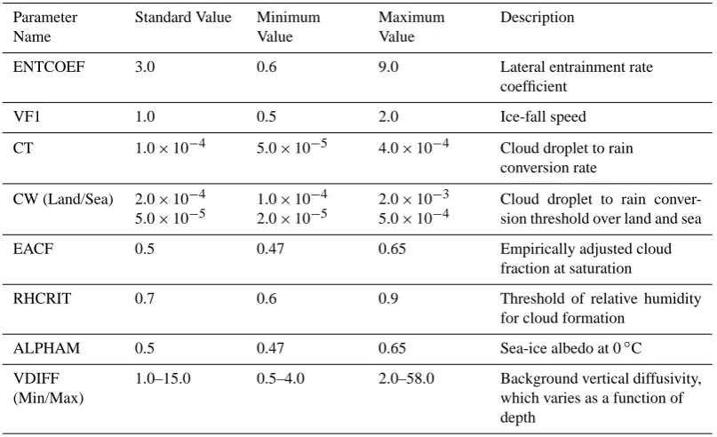
Table 1. Shows a list of the eight parameters perturbed in the experiment. Shown are the value of the parameter in the standard configuration,

the minimum and maximum for the parameter range, and a short description of that parameter.

Parameter Name

Standard Value Minimum Value

Maximum Value

Description

ENTCOEF 3.0 0.6 9.0 Lateral entrainment rate

coefficient

VF1 1.0 0.5 2.0 Ice-fall speed

CT 1.0×10−4 5.0×10−5 4.0×10−4 Cloud droplet to rain conversion rate

CW (Land/Sea) 2.0×10−4 5.0×10−5

1.0×10−4 2.0×10−5

2.0×10−3 5.0×10−4

Cloud droplet to rain conver-sion threshold over land and sea

EACF 0.5 0.47 0.65 Empirically adjusted cloud

fraction at saturation

RHCRIT 0.7 0.6 0.9 Threshold of relative humidity

for cloud formation

ALPHAM 0.5 0.47 0.65 Sea-ice albedo at 0◦C

VDIFF (Min/Max)

1.0–15.0 0.5–4.0 2.0–58.0 Background vertical diffusivity, which varies as a function of depth

the sections of each parameter, ensuring that there is no rep-etition, and giving good univariate separation between mem-bers. There are many possible latin hypercubes which satisfy these conditions and a better sampling is possible with the maximin latin hypercube approach. Maximin latin hypercube sampling adds the requirement that each point drawn must be as far from previous points as possible, thus ensuring a greater multivariate separation of the ensemble members. At this stage each point is defined as a small region of parame-ter space between the minima and maxima of its respective parameter sections. To get a definitive value for each of the point’s parameter co-ordinates a random value between the minimum and maximum of each section of each parameter is found in turn. Thus, we have 200 well-spaced parameter value drawn from across the 8 dimensional parameter space.

2.3 Experimental setup

To select members for our final ensemble, we applied a low-cost selection criterion to these initial 200 members. Instead of running each one of the 200 ensemble members for several hundred years to equilibrium, we only ran them for 20 yr. We then projected the equilibrium temperature of the model runs using the approach of Gregory et al. (2004) and discarded all ensemble members that had projected temperature outside a plausible temperature range. All simulations were started from the end of a many thousand years long pre-industrial spinup of the standard version of HadCM3 (standard model), i.e. with standard parameter values. Around half of the sim-ulations failed to complete these first 20 yr and these failed

members could not be used for further simulations. HadCM3 is known to be not entirely stable across its parameter space (Rougier et al., 2009), and without flux-adjustment some oth-erwise stable simulations have been found to give a simula-tion so unrealistic that they eventually became numerically unstable (Murphy et al., 2004).

To make the equilibrium temperature response projections, we assume that the change in parameters caused an instan-taneous change in radiative forcing, an approach which has previously been applied to perturbed parameter ensembles (Joshi et al., 2010; Shiogama et al., 2012). The projection of temperature and the initial radiative forcing is made from a linear regression of the change in temperature and the change in TOA radiative imbalance from the standard model’s con-trol mean, in the manner of Gregory et al. (2004). Note that not all models exhibit radiative balance in equilibrium, some members of the CMIP3 ensemble show persistent ra-diative imbalances of up to 4.0 W m−2, if so it is necessary to project the equilibrium temperature response using the TOA radiative imbalance anomaly from the standard model. HadCM3 has only a small persistent TOA radiative imbal-ance of−0.13 W m−2, and so we adopted the absolute TOA radiative imbalance. We kept only members which were pro-jected to have equilibrium pre-industrial global-mean tem-perature within 2◦_{C of the estimated pre-industrial}

tempera-ture of 13.6◦_{C (Jones et al., 1999; Brohan et al., 2006), which}

(5)

Projected Temperature and Radiative Forcing

-15 -10 -5 0 5 10 15 20 25 Projected Temperature Change (o_C)

-35 -30 -25 -20 -15 -10 -5 0 5 10 15

Estimated Intitial Radiative Forcing (Wm

-2)

Projected and Measured Temperature

-4 -3 -2 -1 0 1 2 3 4

Projected Temperature Change (o

C) -4

-3 -2 -1 0 1 2 3 4

-4 -3 -2 -1 0 1 2 3 4

Measured Temperature Change (

oC)

Projected Temperature and Radiative Forcing

-5 -4 -3 -2 -1 0 1 2 3 4 5 Projected Temperature Change (o_C)

-8 -7 -6 -5 -4 -3 -2 -1 0 1 2 3 4 5 6 7 8

Estimated Intitial Radiative Forcing (Wm

-2)

a b

c

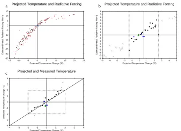
Fig. 1. Projections of equilibrium temperature and initial radiative forcing for the initial ensemble generated by applying the Gregory et

al. (2004) approach to 20 yr of pre-industrial simulation (a, b). Panel (b) shows the acceptable range of temperatures with dashed lines, i.e. within±2◦C of the observed pre-industrial temperature of 13.6◦C (Brohan et al., 2006; Jones et al., 1999). Panel (c) shows a comparison between the projected temperature and the simulated temperature at the end of the 800 yr control run. Simulations which completed the first 20 yr are shown in black and those which failed to complete are shown in red, the large green and black point is for the standard model, the crosses in (b) and (c) show runs which were too warm or cold. The projection method failed for some runs which are shown in blue where the blue dot shows the temperature and radiative imbalance of the last simulated year rather than the projection.

CMIP3 ensemble (i.e.−1.8◦C) and similar to the spread of 3.3◦C (Meehl et al., 2007b).

The members which passed this selection criterion formed the final PPE ensemble and were used for further simula-tions. As we are modifying the ocean and atmosphere of the model it will take thousands of years for the model to equi-librate fully. Due to computational constraints we cannot run the model this long, and so we follow Collins et al. (2007), and run a 500 yr spinup to allow some degree of adjustment to the altered conditions. After the spinup 2 further simula-tions were started, a 300 yr pre-industrial control run and a 150 yr simulation with an instantaneous quadrupling of CO2

(4*CO2).

3 Results

3.1 Initial selection on projected temperature response

The initial selection of the PPE was based on the projected temperature, Fig. 1a and b shows the projected temperature and estimated initial TOA radiative imbalance of the ini-tial 200 members. A large number of the simulations failed

to complete, but there was no clear relation between fail-ure to complete this first 20 yr and any individual param-eter. Around three quarters of the simulations which com-pleted the 20 yr pre-industrial control simulations had very large changes in TOA radiative balance and were projected to warm or cool rapidly, deviating greatly from the observed global-mean pre-industrial temperature. Figure 1c shows the projected temperature from the first 20 yr and the tempera-ture after 800 yr of pre-industrial control run for each of the 27 members which were projected to be within±2.0◦C of the observed pre-industrial temperature of 13.6◦C (Brohan et al., 2006; Jones et al., 1999). Most of the members of the PPE are close to their respective projected temperatures, but two warmer members, and a single cold member, are clearly outside of the range, with three further runs within 0.2◦C of the target range. Of the 27 members selected by the Gregory method≈80 % remained within the target window and most are within a few tenths of a degree of their projected values. The application of this approach avoided the need to run the tens of initially rejected members to equilibrium, saving sub-stantial amounts of computing time.

(6)

Surface Air Temperature

0 100 200 300 400 500 600 700 800 Year

10 11 12 13 14 15 16 17 18

Temperature (

oC)

Radiative Imbalance TOA

0 100 200 300 400 500 600 700 800 Year

-2.0 -1.5 -1.0 -0.5 0.0 0.5 1.0 1.5 2.0 2.5 3.0 3.5 4.0

Radiative Imbalance (Wm

-2)

Precipitation

0 100 200 300 400 500 600 700 800 Year

2.5 2.6 2.7 2.8 2.9 3.0 3.1 3.2 3.3 3.4 3.5

Precipitation (mmDay

-1)

Sea-Ice Area

0 100 200 300 400 500 600 700 800 Year

0.0 5.0 10.0 15.0 20.0 25.0 30.0 35.0 40.0

Sea-Ice Area (10

6 km 2)

a b

c d

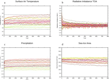
Fig. 2. Evolution over the course of the 800 yr pre-industrial control simulation of the global annual means of surface air temperature (a),

top-of-atmosphere radiative balance (b), precipitation (c) and annual-mean sea-ice area (d). The standard version of HadCM3 is plotted with a thick gray line.

additional 6 failed members. The failed members will be re-tained, but shown only in plots that illustrate the role of the parameters. Supplement Table 1 lists the parameter values and the pre-industrial temperature anomaly from observa-tions of each of the members of the PPE with the members which failed the selection criterion marked.

3.2 Pre-industrial spinup

Overall, we ran 800 yr of pre-industrial conditions with the final ensemble of 21 successful and 6 failed members. Fig-ure 2 shows the evolution of a number of variables over the course of the 800 yr pre-industrial control runs, note that the same colour scheme is used throughout this study to aid the identification of ensemble members across plots. Figure 2a and b show that most members of the PPE behave as if an instantaneous radiative forcing had been applied, in other words, they follow an asymptotic approach to a new equi-librium temperature and the radiative imbalance is decaying to zero. One member has a markedly higher radiative imbal-ance which is at 0.5 W m−2at the end of the control run but remains within the target temperature range after 800 yr. The change in precipitation, Fig. 2c, shows a rapid adjustment to the altered atmospheric conditions followed by a temperature driven change in precipitation (Bala et al., 2010). The sea-ice area, Fig. 2d, changes quite significantly, with the warmer

members losing up to a third of their sea-ice, and some mem-bers gaining sea-ice area.

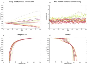
Figure 3a shows that the deep ocean has not adjusted fully to the parameter perturbations by the end of the pre-industrial control; all the members of the ensemble show deep-ocean temperature trends which change little over the 800 yr control run. In fact, even the standard HadCM3 simu-lation, still shows a slight cooling. Figure 3b shows the evo-lution of the maximum meridional overturning circulation in the Atlantic; most members remain close to the standard model’s condition with an overturning strength of≈18 Sv, but 3 of the members show increased overturning of around

(7)

Deep Sea Potential Temperature

0 100 200 300 400 500 600 700 800 Year

0.0 0.2 0.4 0.6 0.8 1.0 1.2 1.4 1.6 1.8 2.0

Temperature (

oC)

Max Atlantic Meridional Overturning

0 100 200 300 400 500 600 700 800 Year

10 15 20 25 30 35

Overturning (Sv)

Temperature

-5 0 5 10 15 20 25

Temperature (o

C) 0.0

0.5 1.0 1.5 2.0 2.5 3.0 3.5 4.0 4.5 5.0

0.0 0.5 1.0 1.5 2.0 2.5 3.0 3.5 4.0 4.5 5.0

Depth (km)

Salinity

-2.0 -1.5 -1.0 -0.5 0.0 0.5 1.0 Salinity (PSU-35)

0.0 0.5 1.0 1.5 2.0 2.5 3.0 3.5 4.0 4.5 5.0

Depth (km)

a b

c d

Fig. 3. Evolution of the global annual means of potential temperature at a depth of 2700 m (a), maximum Atlantic overturning (b) over the

course of the 800 yr pre-industrial control simulation. The figure also shows ocean depth profile of annual and area average temperature (c) and salinity (d), averaged over years 501 to 800 of the pre-industrial control. The standard version of HadCM3 is plotted with a thick gray line.

most strongly associated with the value of the VDIFF param-eter rather than the control temperature, with the members with the highest values of VDIFF showing a large increase in overturning whereas the members with a standard or low value of VDIFF showing little change. This strong response of Atlantic overturning to changes in VDIFF in HadCM3 was also found by Brierley et al. (2010).

The effect of the perturbed atmospheric and sea-ice pa-rameters on the HadCM3 model have been explored in detail by a number of other studies (Collins et al., 2006; Murphy et al., 2004; Sanderson et al., 2008a; Knight et al., 2007), as have the effects of the perturbed ocean parameter (Collins et al., 2007; Brierley et al., 2010), and so the interested reader should refer to these for further information. However, we note here a number of relevant correlations we find between some parameters and the resulting pre-industrial climate. We find that the ENTCOEF and VF1 parameters that have pre-viously been found to have the largest role in controlling cli-mate sensitivity in the HadCM3 model are also found to exert significant control over the equilibrium pre-industrial tem-perature (Rougier et al., 2009; Sanderson et al., 2008a), with low values of both parameters tending to give warmer con-ditions. We also find that higher values of ocean vertical dif-fusivity (VDIFF) are associated with more positive radiative imbalance in the pre-industrial control, despite not directly

affecting the global energy budget. For high values of the VDIFF parameter more energy is absorbed by the ocean (up to≈1.4 W m−2compared with≈0.6 W m−2in the standard model), absorbing energy that would otherwise have warmed the model surface, and vice versa for low values of VDIFF. It seems likely that this association between high values of VD-IFF and higher pre-industrial temperatures is due to VDVD-IFF mitigating the initial rate of temperature change (C. Brier-ley, personal communication, 2011). It has been found that high values of VDIFF cause an increase in the flux of en-ergy into the oceans in the initial years and so may act to keep members, that would have otherwise warmed too fast, close to the observed pre-industrial temperature (Brierley et al., 2010). We also note that the sea-ice minimum albedo pa-rameter (ALPHAM) has a much smaller effect than surface air temperature on the pre-industrial sea-ice fraction.

3.3 Comparison of the PPE with ERA-40 and the CMIP3 ensemble

(8)

PPE - Surface Air Temperature

-90 -80 -70 -60 -50 -40 -30 -20 -10 0 10 20 3040 50 60 7080 90 Latitude

-50 -40 -30 -20 -10 0 10 20 30

Temperature (Celsius)

PPE - Precipitation

-90 -80 -70 -60 -50 -40 -30 -20 -10 0 1020 30 4050 60 70 8090 Latitude

0.0 1.0 2.0 3.0 4.0 5.0 6.0 7.0 8.0 9.0

Precipitation (mmday

-1)

PPE - ERA-40 anomaly - Surface Air Temperature

-90 -80 -70 -60 -50 -40 -30 -20 -10 0 10 20 3040 50 60 7080 90 Latitude

-14.0 -12.0 -10.0 -8.0 -6.0 -4.0 -2.0 0.0 2.0 4.0 6.0 8.0 10.0

Temperature (Celsius)

PPE - ERA-40 anomaly - Precipitation

-90 -80 -70 -60 -50 -40 -30 -20 -10 0 1020 30 4050 60 70 8090 Latitude

-3.5 -3.0 -2.5 -2.0 -1.5 -1.0 -0.5 0.0 0.5 1.0 1.5 2.0 2.5 3.0

Precipitation (mmday

-1)

a b

c d

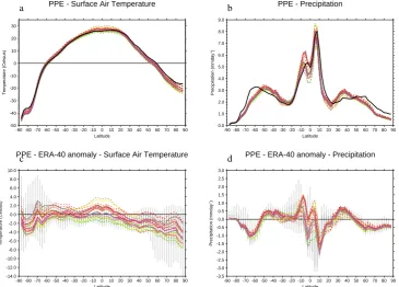
Fig. 4. The zonal-mean surface air temperature (a) and precipitation (b) for the PPE simulations with the ERA-40 1961–1990 mean plotted

for comparison. The zonal-mean anomaly between each member of the PPE and the ERA-40 mean for surface air temperature (c) and precipitation (d). The standard version of HadCM3 is plotted in dark gray and the ERA-40 mean is plotted in black. In (c) and (d) the range for the CMIP3 ensemble is plotted with light gray bars and the standard deviation of the CMIP3 ensemble around the ensemble mean is plotted with darker gray bars.

broadly similar to the ERA-40 dataset, however there are no-ticeable differences south of the equator and polewards of the sub-tropical dry regions. To put the differences between the PPE and the ERA-40 dataset in context, Fig. 4c and d show the anomaly from the ERA-40 dataset for both the PPE en-semble and the CMIP3 enen-semble for SAT and precipitation, respectively. Most members of both ensembles are colder than the ERA-40 dataset, particularly at high northern lati-tudes, as one would expect from the warming that occurred between the pre-industrial and the late 20th century. Some members of the PPE are up to 4.0◦C warmer than the ERA-40 dataset in the Tropics, substantially warmer than any of the CMIP3 members. The low-latitude ocean heat transport in HadCM3 has been found to be relatively ineffective and on long timescales this can effectively act as a positive feedback on radiative imbalances at low-latitudes (Vellinga and Wu, 2008), which could explain why the anomalous behaviour is limited to this region. Both the PPE and CMIP3 ensembles show reduced precipitation at high latitudes compared with the ERA-40 dataset, which again fits with the changes ex-pected between the pre-industrial and the late 20th century.

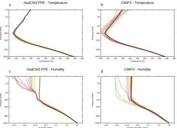
Most of the parameters that were perturbed in the PPE were related to uncertain atmospheric processes, particularly convective and cloud processes, and so one would expect dif-ferences throughout the atmospheric column. Figure 5 shows

a comparison between the ERA-40 1961–1990 mean verti-cal temperature and specific humidity profiles and both the PPE and the CMIP3 ensemble (Meehl et al., 2007b). The PPE follows the vertical temperature profile of the ERA-40 dataset, with all members remaining within≈5◦C through-out whereas the CMIP3 ensemble shows a wider spread par-ticularly at higher altitudes where models differ by up to 10◦C, see Fig. 5a and b. Both the PPE and the CMIP3 ensem-ble follow the ERA-40 humidity profile with humidity de-clining with altitude until it reaches around a few ppm at the tropopause. The ERA-40 dataset and many CMIP3 members show almost constant humidity throughout the stratosphere whereas some CMIP3 members and all PPE members show a continuing decline in humidity with altitude. All members of the PPE thus have a stratospheric water vapour content that is of the order of one tenth of the ERA-40 value.

(9)

HadCM3 PPE - Temperature

200 210 220 230 240 250 260 270 280 290 300 Temperature (K)

1000 500 200 100 50 20 10

Pressure (hPa)

CMIP3 - Temperature

200 210 220 230 240 250 260 270 280 290 300 Temperature (K)

1000 500 200 100 50 20 10

Pressure (hPa)

HadCM3 PPE - Humidity

1e-5 1e-4 1e-3 1e-2 0.1 1.0 10 Humidity (g/Kg)

1000 500 200 100 50 20 10

Pressure (hPa)

CMIP3 - Humidity

1e-5 1e-4 1e-3 1e-2 0.1 1.0 10 Specific Humidity (g/Kg)

1000 500 200 100 50 20 10

Pressure (hPa)

a b

c d

Fig. 5. The temperature (a, b) and specific humidity (c, d) throughout the atmospheric column for the PPE simulations and the CMIP3

ensemble. The standard version of HadCM3 is plotted in dark gray for the PPE simulations and the ERA-40 1961–1990 mean is plotted in black. Note that for the PPE cells below ground level, the values are extrapolated using an average lapse rate and included in the level mean.

difference (i.e. the average from 60◦N to 90◦N and be-tween 30◦_{S and 30}◦_{N), global mean precipitation,}

maxi-mum overturning strength in the Atlantic, and global-mean pre-industrial humidity at 100 hPa and at 10 hPa. After 800 yr of pre-industrial control 6 of the PPE members were found to fall outside the target temperature of 13.6±2◦C. The av-erage pole to equator temperature difference for the PPE is 42.0◦C which is greater than the ERA-40 average of 39.6 for the period 1961–1990, however this may be partly due to the warming of the 20th century which will be greatest at high latitudes reducing the pole to equator temperature range. For the Atlantic overturning circulation we find a number of members show a substantially stronger overturning than the observed value of 18.7 Sv reported by Rayner et al. (2011), but only 2 accepted members of the PPE exceed the range of 12 to 24 Sv, given as the largest observational range in the IPCC Assessment Report 4 (Meehl et al., 2007a).

As was shown in Fig. 5 the specific humidity of the PPE is fairly close to the ERA-40 reanalysis at 100 hPa with an average value that is 70 % of the ERA-40 value but at 10 hPa the PPE has between 30 % and less than 1 % of the ERA-40 value. As absorption of longwave radiation scales ap-proximately with the logarithm of the concentration of wa-ter vapour (Forswa-ter and Shine, 2002; IPCC, 2007), one could expect large changes in the water vapour greenhouse ef-fect in the PPE (Held and Soden, 2000; Forster and Shine,

2002; Joshi et al., 2010). However, the absolute water vapour content is extremely low and major changes in the strato-spheric radiation budget would be reflected in the upper at-mospheric temperatures (Forster and Shine, 2002), but these have changed little from the standard model values, see Fig. 5a. Furthermore, the CMIP3 ensemble also includes many models with very dry stratospheres and this does not seem to be a critical shortcoming in these models.

Finally, as was shown in Fig. 4, the zonal mean clima-tology of the PPE generally compares well to the ERA-40 reanalysis, although some exceptions to this are found in the zonal temperature where some accepted members stand out clearly from the ERA-40 reanalysis and are well beyond the CMIP3 ensemble range. It is clear that the PPE shows a narrower range of behaviour than the CMIP3 ensemble and that the PPE shares many biases with the standard HadCM3 model configuration. Overall, we judge that the 21 accepted members of the PPE are plausible representations of the pre-industrial climate, and we retain all members which passed the initial temperature selection criterion.

3.4 Elevated CO2experiments

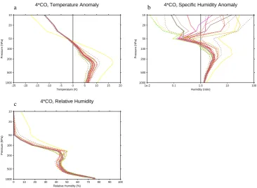
Figure 6 shows the change in the vertical profile of some atmospheric variables at the end of the 150 yr 4*CO2

(10)

4*CO2 Temperature Anomaly

-25 -20 -15 -10 -5 0 5 10 15 20 Temperature (K)

1000 500 200 100 50 20 10

Pressure (hPa)

4*CO2 Specific Humidity Anomaly

1e-2 0.1 1.0 10 100

Humidity (ratio) 1000

500 200 100 50 20 10

1000 500 200 100 50 20 10

Pressure (hPa)

4*CO2 Relative Humidity

0 10 20 30 40 50 60 70 80 90 100 Relative Humidity (%)

1000 500 200 100 50 20 10

Pressure (hPa)

a b

c

Fig. 6. The response of the PPE at 4*CO2throughout the atmospheric column; the anomaly between 4*CO2and the pre-industrial control

for temperature (a); the ratio of specific humidity between 4*CO2and the pre-industrial control (b); and the absolute relative humidity at

4*CO2(c). The standard version of HadCM3 is shown in dark gray. Note that FOR cells below ground level the values are extrapolated using

an average lapse rate and included in the level mean.

(IPCC, 2007), i.e. a warming in the troposphere, a rise of the tropopause, and a cooling of the stratosphere. There is a wide spread of temperature response, but all members show a peak warming in the mid-troposphere which is roughly 50 % greater than the surface warming. At higher altitudes most members of the PPE show the same cooling of≈12◦_C

despite a broader range of surface temperature responses,

≈6±1.5◦C; however, one accepted member shows a sur-face warming of around 11◦C and a high altitude cooling of around 18◦C, much greater than any other model. Figure 6b shows the change in specific humidity; up to 100 hPa the hu-midity increases for all members in a similar way, with the warmer runs showing a greater increase in humidity. How-ever, at higher altitudes there is a very broad range of re-sponse with many members, including the standard model, showing humidity decreasing to a tenth, or even a hundredth, of the pre-industrial value and others showing a ten to a hun-dred fold increase in humidity. However, it is the absolute hu-midity that determines the magnitude of the radiative contri-bution of high altitude humidity and all but the two warmest PPE members remain below the ERA-40 1961–1990 strato-spheric value of≈3 ppm. The warmest PPE member shows a specific humidity of≈10 ppm, i.e. more than three times greater than the 1961–1990 ERA-40 stratospheric humidity. For most members over most of the atmospheric column the

absolute change in relative humidity is less than 5 %, exclud-ing around 150 hPa, where changes in tropopause height are evident. The warmest and second warmest accepted mem-bers (the solid yellow and dashed dark brown lines) stand out in the specific and relative humidity plots at altitudes above 100 hPa, showing specific humidity levels of order 100 and 10 times greater than the mean response and relative humidi-ties of order 10 % and 1 % where other models show effec-tively 0 % relative humidity, see Fig. 6c.

(11)

Pre-Industrial 1 2 3 4 5 6 7 8 9

1011142224231925182017 1613 12 21 15 26

0

ENTCOEF < 2.0 2.0 < ENTCOEF < 2.5 ENTCOEF > 2.5 Standard

0.6 1.2 1.8 2.4 3.0 3.6 4.2 4.8 5.4 6.0 6.6 7.2 7.8 8.4 9.0

ENTCOEF 0.0 2.0 4.0 6.0 8.0 10.0 12.0 14.0 16.0 0.0 2.0 4.0 6.0 8.0 10.0 12.0 14.0 16.0

Specific Humidity at 30 hPa (ppm)

4*CO2 1 2 3 4 5 6 7 8 9 10 11 12 13 14 15 16 17 18

19 20 21 222423

25 26

0

0.6 1.2 1.8 2.4 3.0 3.6 4.2 4.8 5.4 6.0 6.6 7.2 7.8 8.4 9.0

ENTCOEF 0.0 2.0 4.0 6.0 8.0 10.0 12.0 14.0 16.0 0.0 2.0 4.0 6.0 8.0 10.0 12.0 14.0 16.0

Specific Humidity at 30 hPa (ppm)

4*CO2 1 2 3 4 5 6 7 8 9 10 11 12 13 14 15 16 17 18

1920 21 222423 25

26

0

0.6 1.2 1.8 2.4 3.0 3.6 4.2 4.8 5.4 6.0 6.6 7.2 7.8 8.4 9.0

ENTCOEF 0.0 2.0 4.0 6.0 8.0 10.0 12.0 14.0 16.0 18.0 20.0 22.0 0.0 2.0 4.0 6.0 8.0 10.0 12.0 14.0 16.0 18.0 20.0 22.0

Relative Humidity at 30 hPa (%)

4*CO2 Anomaly 1 2 3 4 5 6 7 8 9 10 11 12 13 14

15171816 1922202321

24 25

26

0

0.0 1.0 2.0 3.0 4.0 5.0 6.0 7.0 8.0 9.0 10.0 11.0 12.0

Temperature Change (o_C) -2.0 0.0 2.0 4.0 6.0 8.0 10.0 12.0 14.0 -2.0 0.0 2.0 4.0 6.0 8.0 10.0 12.0 14.0

Specific Humidity Change at 30 hPa (ppm)

a b

c d

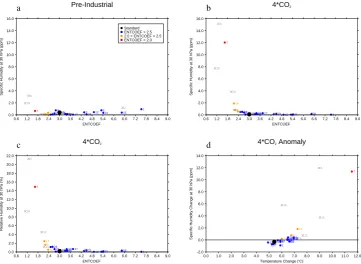
Fig. 7. The specific humidity at 30 hPa for the pre-industrial (a) and 4*CO₂(b) as a function of ENTCOEF, the relative humidity at 30 hPa for

4*CO2as a function of ENTCOEF (c), and the change in specific humidity at 30 hPa and temperature between the 4*CO2and pre-industrial

simulations (d). The standard model is shown as a larger black dot and failed runs were included in this plot as gray crosses to make clearer the role of the parameter. Values of ENTCOEF are also indicated with colours as indicated in the legend.

4*CO2simulation; members with a value of ENTCOEF

be-low about 2.5 show specific humidities of between 0.5 and 15 ppm whereas others show very low specific humidities of less than 0.5 ppm (Joshi et al., 2010; Sanderson et al., 2008a; Sanderson, 2011). ENTCOEF also affects the relative humid-ity of the stratosphere which increases sharply for values of ENTCOEF below about 2.5 in the 4*CO2 experiment, see

Fig. 7c. Figure 7d shows that generally the members with the largest changes in high altitude humidity also show the largest increases in temperature at 4*CO2.

Figure 8a shows how TOA radiative imbalance and tem-perature change evolve over the course of the 4*CO2

ex-periment for the PPE ensemble. The method of Gregory et al. (2004) involves carrying out a regression on the joint evolution of temperature and radiative imbalance and is ex-pected to provide an estimate of the initial radiative forc-ing perturbation and a final equilibrium temperature after only a few years or decades of such an instantaneous forc-ing experiment. Most ensemble members roughly follow the expected linear trend, although there is a common drift to higher temperatures towards the end of the runs as was seen by Gregory et al. (2004) for coupled models. The warmest ensemble member does not follow a linear evolution of TOA radiative imbalance and temperature at all, instead after a number of years the radiative imbalance ceases to reduce whilst temperature continues to rise at≈0.4 K per decade

over the last 50 yr. This nonlinear climate response is also seen in a number of the failed ensemble members, i.e. those which fell outside of the temperature limits after 800 yr of pre-industrial control. The projected equilibrium tempera-tures of the 4*CO2simulations (4*CS) are shown in Fig. 8b,

these are found by applying the Gregory method to the entire 150 yr timeseries. This long fitting period was applied to cap-ture some of the deviation that the members with the great-est warming show. Most accepted ensemble members have a 4*CS in the range of 6.5–10.5◦C, with the warmest accepted member having an estimated 4*CS of 35◦C, although this is likely an underestimate due to the breakdown of the lin-ear relation between increasing temperatures and decreasing TOA radiative imbalance. We also note a weak correlation between high pre-industrial temperature and climate sensi-tivity.

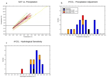
Figure 9a shows how precipitation and temperature evolve over the course of the 4*CO2 experiment for the PPE

(12)

SAT vs. TOA Radiative Imbalance

0.0 1.0 2.0 3.0 4.0 5.0 6.0 7.0 8.0 9.0 10.0 11.0 12.0 Temperature (o

C) 0.0

1.0 2.0 3.0 4.0 5.0 6.0 7.0

0.0 1.0 2.0 3.0 4.0 5.0 6.0 7.0

Radiative Imbalance (Wm

-2)

4*CO2 - Projected Temperature Change

6.0 6.5 7.0 7.5 8.0 8.5 9.0 9.5 10.0 10.5 11.0 11.5 12.0 >12 Temperature Change (o

C) 0

1 2 3 4 5 6

0 1 2 3 4 5 6

Number

a b

Fig. 8. The evolution of the TOA radiative imbalance and temperature over the full 150 yr of the 4*CO2simulation (a) and a histogram of

projections of the equilibrium temperature for the 4*CO2simulation (b). The projections of equilibrium temperature are made using the

Gregory method for all 150 yr of the simulations. The members which failed the pre-industrial temperature selection are included as gray lines in panel a. All changes are relative to the pre-industrial control simulations.

SAT vs. Precipitation

0.0 1.0 2.0 3.0 4.0 5.0 6.0 7.0 8.0 9.0 10.0 11.0 12.0 Temperature (o

C) -6.0

-4.0 -2.0 0.0 2.0 4.0 6.0 8.0 10.0 12.0 14.0

-6.0 -4.0 -2.0 0.0 2.0 4.0 6.0 8.0 10.0 12.0 14.0

Precipitation (%)

4*CO2 - Precipitation Adjustment

-7.4 -7.2 -7.0 -6.8 -6.6 -6.4 -6.2 -6.0 -5.8 -5.6 -5.4 -5.2 -5.0 -4.8 -4.6 -4.4 Precipitation Change (%)

0 1 2 3 4 5 6

Number

4*CO2 - Hydrological Sensitivity

1.0 1.1 1.2 1.3 1.4 1.5 1.6 1.7 1.8 1.9 2.0 2.1 2.2 2.3 2.4 2.5 Hydrological Sensitivity (%o

C-1

) 0

1 2 3 4 5 6

0 1 2 3 4 5 6

Number

a b

c

Fig. 9. The evolution of percentage precipitation change and temperature change over the full 150 yr of the 4*CO2simulation relative to

the pre-industrial averages (a), and histograms of the estimated precipitation adjustment (b) and hydrological sensitivity (c) for the 4*CO2

simulation. Linear fits to the first 50 yr of each simulation are used to calculate the precipitation adjustments, which are found from the intercept where1SAT=0, and the hydrological sensitivities, which are found from the gradients of the linear fits.

type of forcing, and a more or less independent slow compo-nent, that depends on the global mean temperature (Andrews et al., 2010; Bala et al., 2010). This slow, temperature-driven, component has been called the “hydrological sensitivity” and is measured in percentage change per degree of warming (%◦C−1)(Bala et al., 2010; Andrews et al., 2010). Calcu-lating these values by applying a linear fit to the first 50 yr of the 4*CO2experiment we find that the PPE shows a range

of both fast and slow behaviour to the 4*CO2 forcing with

a precipitation adjustment of between−4.8 to−7.0 %, and a hydrological sensitivity of between 1.8 to 2.3 %◦C−1 (ex-cepting the warmest accepted member which has a value of less than 1.6 %◦C−1), see Fig. 9b and c. At 2*CO2Andrews

(13)

with our HadCM3 PPE results they find a hydrological sensi-tivity of 2.2 %◦_C−1_{and a precipitation adjustment of 3.0 %}

(roughly half the 4*CO2value shown here) for the HadSM3

model.

4 Discussion

To produce this non-flux adjusted perturbed parameter en-semble of HadCM3, an initial enen-semble was produced us-ing a maximin latin hypercube samplus-ing approach and then a simple selection criteria was applied, based on the pro-jected temperature response of the members from a 20 yr pre-industrial simulation. This approach allowed a large num-ber of initial parameter combinations to be screened to ex-clude ensemble members that would produce an unrealisti-cally warm or cold pre-industrial climate. This projection ap-proach, based on the Gregory method (Gregory et al., 2004), was largely successful. Only 6 of the 27 members of the ensemble members failed to remain within the target tem-perature range of 13.6±2.0◦C after 800 yr of pre-industrial simulation (see Fig. 1c), corresponding to a success rate of 80 %, and those that failed were mostly within a few tenths of a degree of the target range. To aid future applications of this approach we highlight a number of issues with this approach. Firstly, many GCMs do not have a perfect radia-tive balance in equilibrium as they contain energy sources or sinks of up to a few W m−2and so we suggest using the anomaly in TOA radiative imbalance rather than absolute ra-diative imbalance for making these projections (Mauritsen et al., 2012). Secondly, internal variability affects projections based on short timeseries, but longer runs or additional short simulations obviously increase computational cost and we judge that 20 yr was a good compromise. Thirdly, we as-sumed that a change in parameter values would be realised as an instantaneous change in radiative forcing and a change in the feedback processes of the model, but this is not neces-sarily the case. Analysis by Joshi et al. (2010), indicate that perturbations of the ENTCOEF parameter induce changes in the climate that do not follow the linear relation between temperature and radiative forcing that is commonly assumed (Gregory et al., 2004). Finally, if ocean parameters are per-turbed the energy balance between atmosphere and ocean can change independently of the TOA radiative imbalance (Brierley et al., 2010). Our results suggest that the perturba-tion of the vertical ocean diffusivity parameter lead to an ad-justment of the ocean-atmosphere energy balance, which af-fected our short-term temperature projections. Despite these difficulties, we believe our use of short-term projections us-ing the Gregory et al. (2004) approach has been very success-ful, as running all 200 initial members for 800 yr would have required≈160 000 model years as opposed to the≈25 000 model years required with our approach.

The pre-industrial climates of the PPE were evaluated on the basis of a comparison to the ERA-40 dataset and by

consideration of the spread of the CMIP3 ensemble, see Sect. 3.3. Most PPE members show behaviour that is rea-sonably close to the ERA-40 data, but a number of mem-bers showed tropical temperatures up to 4◦C warmer than the ERA-40 data and some showed high values for the Atlantic overturning circulation. All members of the PPE seemed to share some biases with the standard version of the HadCM3 model. This under-dispersion in the range of behaviour in the PPE is a common problem for PPEs, particularly those which perturb only a limited number of parameters (Yoko-hata et al., 2012). Overall, the initial selection criteria ap-pears to have been very successful in that it removed all the members of the PPE which exhibited pre-industrial climatic conditions that are clearly implausible, but the small number of perturbed parameters has limited the range of behaviour within the PPE.

We find very high climate sensitivities for PPE mem-bers with low values of the ENTCOEF parameter, includ-ing one accepted member, and a number of the members which failed the temperature selection criterion, which show a clearly nonlinear response with unchecked warming in the later years of the 4*CO2experiment, see Fig. 8. The

mech-anism behind this unchecked warming has not been defini-tively identified, but one plausible hypothesis presented in Sanderson (2011) is that the large increases in upper atmo-spheric humidity in response to warming in the warmest member constitutes a very large, positive, clear-sky longwave feedback which comes to dominate at higher temperatures. The climate sensitivity of HadCM3 has been found to rise rapidly for ENTCOEF values below the standard value of 3.0 (see Fig. 6 of Sanderson et al., 2008a and Fig. 6 of Rougier et al., 2009), and here we find that the stratospheric humidity response to elevated CO2also rises rapidly below ENTCOEF

values of about 2.5. Most GCMs simulate a weak strato-spheric humidity response to warming and small changes in relative humidity throughout the atmospheric column (Col-man, 2001; Stuber et al., 2005), which is backed up by ob-servations of recent warming (IPCC, 2007).

(14)

question of how should a nonlinear climate response be in-terpreted? Are such runaway climate responses plausible? Or should PPE methods include a test of the climate response to elevated CO2concentrations which screens out members

with nonlinear climate responses? We would suggest that the PPE members which produced climate sensitivity estimates towards the extreme upper end may be suspect; either under-estimating climate sensitivity if such nonlinear climate re-sponses in HadCM3 are plausible or over-estimating climate sensitivity if they are implausible and should be excluded. We thus agree with the conclusion of Joshi et al. (2010) that the very high climate sensitivities found for low values of ENTCOEF are very unlikely in light of the observed re-sponse to warming. We suggest that future PPEs of HadCM3 should test whether a linear climate response best describes the response of the ensemble members and should consider restricting the range of ENTCOEF from 0.6–9.0 to 2.0–9.0 to mitigate these issues.

5 Conclusions

This study presents the methodology and some initial results from a perturbed parameter ensemble (PPE) of a non-flux adjusted, fully-coupled CMIP3-era GCM. The purpose has been to create a modestly-sized PPE to explore the effects of parametric uncertainty on climate and paleo-climate exper-iments. 200 different versions of the HadCM3 model were generated with 8 continuous parameters varied. 21 ensemble members of the HadCM3 model (Gordon et al., 2000), in-cluding the standard configuration, were selected from these 200 using an estimation of the equilibrium pre-industrial temperature to constrain the ensemble, i.e. models with pro-jected temperatures within 13.6±2◦C were kept (Brohan et al., 2006; Jones et al., 1999). However, an additional 6 members which were projected to be within the target tem-perature range were either warmer or colder after the 800 yr control than the target temperature range and thus were ex-cluded from the ensemble. Despite the ocean not reaching equilibrium after 800 yr the pre-industrial control surface cli-matology of the ensemble compares well on the whole to the ERA-40 dataset and the CMIP3 ensemble, except in the Tropics for some members (Meehl et al., 2007b). We find that not using flux-adjustment and instead constraining our en-semble on the pre-industrial equilibrium temperature has not led to a serious curtailment of parameter space as has been suggested previously (Collins et al., 2006). Applying the en-semble to a quadrupled CO2 experiment reinforced earlier

findings of links between low values of the entrainment rate coefficient, large increases in high altitude humidity and high climate sensitivities in HadCM3 (Joshi et al., 2010). In fact, one member with a low value of the entrainment rate coeffi-cient exhibited a clearly nonlinear climate response at 4*CO2

after a few decades, showing a rapid warming without a re-duction in TOA radiative imbalance. This raises the question

of whether the plausibility of ensemble members’ response to elevated CO2 concentrations should be evaluated

along-side historical performance in perturbed parameter ensemble studies.

Supplementary material related to this article is available online at http://www.geosci-model-dev.net/6/ 1447/2013/gmd-6-1447-2013-supplement.zip.

Acknowledgements. P. J. Irvine acknowledges support in the form of a NERC PhD studentship. We acknowledge the CMIP3 mod-elling groups for making their model output available for analysis, the Program for Climate Model Diagnosis and Intercomparison (PCMDI) for collecting and archiving this data, and the WCRP’s Working Group on Coupled Modelling (WGCM) for organising the model data analysis activity. The WCRP CMIP3 multi-model dataset is supported by the Office of Science, US Department of Energy. ECMWF ERA-40 data used in this study have been obtained from the ECMWF Data Server.

Edited by: R. Redler

References

Andrews, T., Forster, P. M., and Gregory, J. M.: A Surface En-ergy Perspective on Climate Change, J. Climate, 22, 2557–2570, doi:10.1175/2008jcli2759.1, 2009.

Andrews, T., Forster, P. M., Boucher, O., Bellouin, N., and Jones, A.: Precipitation, radiative forcing and global temperature change, Geophys. Res. Lett., 37, L14701, doi:10.1029/2010gl043991, 2010.

Bala, G., Caldeira, K., and Nemani, R.: Fast versus slow response in climate change: implications for the global hydrological cy-cle, Clim. Dynam., 35, 423–434, doi:10.1007/s00382-009-0583-y, 2010.

Brierley, C. M., Collins, M., and Thorpe, A. J.: The impact of perturbations to ocean-model parameters on climate and cli-mate change in a coupled model, Clim. Dynam., 34, 325–343, doi:10.1007/s00382-008-0486-3, 2010.

Brohan, P., Kennedy, J. J., Harris, I., Tett, S. F. B., and Jones, P. D.: Uncertainty estimates in regional and global observed tem-perature changes: A new data set from 1850, J. Geophys. Res.-Atmos., 111, D12106, doi:10.1029/2005jd006548, 2006. Cattle, H. and Crossley, J.: MODELING ARCTIC

CLIMATE-CHANGE, Philos. T. Roy. Soc. London Series a, 352, 201–213, 1995.

Collins, M., Booth, B. B. B., Harris, G. R., Murphy, J. M., Sex-ton, D. M. H., and Webb, M. J.: Towards quantifying uncer-tainty in transient climate change, Clim. Dynam., 27, 127–147, doi:10.1007/s00382-006-0121-0, 2006.

(15)

Collins, M., Booth, B., Bhaskaran, B., Harris, G., Murphy, J., Sex-ton, D., and Webb, M.: Climate model errors, feedbacks and forc-ings: a comparison of perturbed physics and multi-model ensem-bles, Clim. Dynam., 36, 1737–1766, doi:10.1007/s00382-010-0808-0, 2010.

Collins, W. J., Bellouin, N., Doutriaux-Boucher, M., Gedney, N., Halloran, P., Hinton, T., Hughes, J., Jones, C. D., Joshi, M., Lid-dicoat, S., Martin, G., O’Connor, F., Rae, J., Senior, C., Sitch, S., Totterdell, I., Wiltshire, A., and Woodward, S.: Develop-ment and evaluation of an Earth-System model – HadGEM2, Geosci. Model Dev., 4, 1051–1075, doi:10.5194/gmd-4-1051-2011, 2011.

Colman, R. A.: On the vertical extent of atmospheric feedbacks, Clim. Dynam., 17, 391–405, doi:10.1007/s003820000111, 2001. Covey, C., AchutaRao, K. M., Cubasch, U., Jones, P., Lam-bert, S. J., Mann, M. E., Phillips, T. J., and Taylor, K. E.: An overview of results from the Coupled Model In-tercomparison Project, Global Planet. Change, 37, 103–133, doi:10.1016/s0921-8181(02)00193-5, 2003.

Cox, P. M., Betts, R. A., Bunton, C. B., Essery, R. L. H., Rown-tree, P. R., and Smith, J.: The impact of new land surface physics on the GCM simulation of climate and climate sensitivity, Clim. Dynam., 15, 183-203, 1999.

Edwards, N. R., Cameron, D., and Rougier, J.: Precalibrating an in-termediate complexity climate model, Clim. Dynam., 37, 1469– 1482, 2011.

Forster, P. M. D. and Shine, K. P.: Assessing the climate impact of trends in stratospheric water vapour, Geophys. Res. Lett., 29, 1086, doi:10.1029/2001gl013909, 2002.

Frame, D. J., Aina, T., Christensen, C. M., Faull, N. E., Knight, S. H. E., Piani, C., Rosier, S. M., Yamazaki, K., Yamazaki, Y., and Allen, M. R.: The climateprediction.net BBC climate change experiment: design of the coupled model ensemble, Philos. T. Roy. Soc. a, 367, 855–870, doi:10.1098/rsta.2008.0240, 2009. Gent, P. R. and McWilliams, J. C.: Isopycnal mixing in ocean

cir-culation models, J. Phys. Oceanogr., 20, 150–155, 1990. Gordon, C., Cooper, C., Senior, C. A., Banks, H., Gregory, J. M.,

Johns, T. C., Mitchell, J. F. B., and Wood, R. A.: The simulation of SST, sea ice extents and ocean heat transports in a version of the Hadley Centre coupled model without flux adjustments, Clim. Dynam., 16, 147–168, 2000.

Gregoire, L., Valdes, P., Payne, A., and Kahana, R.: Optimal tuning of a GCM using modern and glacial constraints, Clim. Dynam., 37, 705–719, doi:10.1007/s00382-010-0934-8, 2010.

Gregory, D. and Rowntree, P. R.: A Mass Flux Convection Scheme with Representation of Cloud Ensemble Characteristics and Stability-Dependent Closure, Mon. Weather Rev., 118, 1483– 1506, 1990.

Gregory, J. M., Ingram, W. J., Palmer, M. A., Jones, G. S., Stott, P. A., Thorpe, R. B., Lowe, J. A., Johns, T. C., and Williams, K. D.: A new method for diagnosing radiative forc-ing and climate sensitivity, Geophys. Res. Lett., 31, L03205, doi:10.1029/2003gl018747, 2004.

Held, I. M. and Soden, B. J.: Water vapour feedback and global warming, Annu. Rev. Energ. Environ., 25, 441–475, doi:10.1146/annurev.energy.25.1.441, 2000.

Houghton, J. T., Ding, Y., Griggs, D. J., Noguer, M., van der Lin-den, P. J., Dai, X., Maskell, K., and Johnson, C.: Climate change 2001: the scientific basis, Cambridge University Press

Cam-bridge, 2001.

IPCC: Climate Change 2007: The Physical Science Basis, in: Cli-mate Change 2007: The Physical Science Basis. Contribution of working Group 1 to the Fourth Assesment Report of the Intergov-ernmental Panel on Climate Change edited by: Solomon, S., Qin, D., Manning, M., Chen, Z., Marquis, M., Averyt, K. B., Tignor, M., and Miller, H. L., Cambridge University Press, Cambridge, 996 pp., 2007.

Jackson, L., Vellinga, M., and Harris, G.: The sensitivity of the meridional overturning circulation to modelling uncertainty in a perturbed physics ensemble without flux adjustment, Clim. Dy-nam., 39, 277–285, doi:10.1007/s00382-011-1110-5, 2012. Jones, P. D., New, M., Parker, D. E., Martin, S., and Rigor, I. G.:

Surface air temperature and its changes over the past 150 years, Rev. Geophys., 37, 173–199, 1999.

Joshi, M. M., Webb, M. J., Maycock, A. C., and Collins, M.: Strato-spheric water vapour and high climate sensitivity in a version of the HadSM3 climate model, Atmos. Chem. Phys., 10, 7161– 7167, doi:10.5194/acp-10-7161-2010, 2010.

Klocke, D., Pincus, R., and Quaas, J.: On Constraining Es-timates of Climate Sensitivity with Present-Day Observa-tions through Model Weighting, J. Climate, 24, 6092–6099, doi:10.1175/2011JCLI4193.1, 2011.

Knight, C. G., Knight, S. H. E., Massey, N., Aina, T., Christensen, C., Frame, D. J., Kettleborough, J. A., Martin, A., Pascoe, S., Sanderson, B., Stainforth, D. A., and Allen, M. R.: Association of parameter, software, and hardware variation with large-scale be-haviour across 57„000 climate models, P. Natl. Acad. Sci. USA, 104, 12259–12264, doi:10.1073/pnas.0608144104, 2007. Masson, D. and Knutti, R.: Climate model genealogy, Geophys.

Res. Lett., 38, L08703, doi:10.1029/2011gl046864, 2011. Mauritsen, T., Stevens, B., Roeckner, E., Crueger, T., Esch, M.,

Giorgetta, M., Haak, H., Jungclaus, J., Klocke, D., Matei, D., Mikolajewicz, U., Notz, D., Pincus, R., Schmidt, H., and Tomassini, L.: Tuning the climate of a global model, J. Adv. Model. Earth Syst., 4, M00A01, doi:10.1029/2012MS000154, 2012.

Meehl, G., Stocker, T., Collins, W., Friedlingstein, P., Gaye, A., Gregory, J., Kitoh, A., Knutti, R., Murphy, J., and Noda, A.: Global climate projections. Chapter 10 in: Climate Change 2007: The Physical Science Basis. Contribution of Working Group I to the Fourth Assessment Report of the Intergovernmental Panel on Climate Change, edited by: Solomon, S. and Qin, D. M., Cam-bridge University Press, CamCam-bridge, United Kingdom, and New York, NY, USA, 996 pp., 2007a.

Meehl, G. A., Covey, C., Delworth, T., Latif, M., McAvaney, B., Mitchell, J. F. B., Stouffer, R. J., and Taylor, K. E.: The WCRP CMIP3 multimodel dataset – A new era in climate change re-search, B. Am. Meteorol. Soc., 88, 1383, doi:10.1175/bams-88-9-1383, 2007b.

Murphy, J. M., Sexton, D. M. H., Barnett, D. N., Jones, G. S., Webb, M. J., and Collins, M.: Quantification of modelling uncertainties in a large ensemble of climate change simulations, Nature, 430, 768–772, doi:10.1038/nature02771, 2004.

(16)

Rayner, D., Hirschi, J. J. M., Kanzow, T., Johns, W. E., Wright, P. G., Frajka-Williams, E., Bryden, H. L., Meinen, C. S., Baringer, M. O., Marotzke, J., Beal, L. M., and Cunningham, S. A.: Moni-toring the Atlantic meridional overturning circulation, Deep-Sea Res. II, 58, 1744–1753, doi:10.1016/j.dsr2.2010.10.056, 2011. Rodwell, M. J. and Palmer, T. N.: Using numerical weather

predic-tion to assess climate models, Q. J. Roy. Meteorol. Soc., 133, 129–146, doi:10.1002/qj.23, 2007.

Rougier, J., Sexton, D. M. H., Murphy, J. M., and Stainforth, D.: Analysing the Climate Sensitivity of the HadSM3 Climate Model Using Ensembles from Different but Related Experiments, J. Cli-mate, 22, 3540–3557, doi:10.1175/2008jcli2533.1, 2009. Sanderson, B. M.: A Multimodel Study of Parametric

Un-certainty in Predictions of Climate Response to Rising Greenhouse Gas Concentrations, J. Climate, 24, 1362–1377, doi:10.1175/2010jcli3498.1, 2011.

Sanderson, B. M., Knutti, R., Aina, T., Christensen, C., Faull, N., Frame, D. J., Ingram, W. J., Piani, C., Stainforth, D. A., Stone, D. A., and Allen, M. R.: Constraints on model response to green-house gas forcing and the role of subgrid-scale processes, J. Cli-mate, 21, 2384–2400, doi:10.1175/2008jcli1869.1, 2008a. Sanderson, B. M., Piani, C., Ingram, W. J., Stone, D. A., and Allen,

M. R.: Towards constraining climate sensitivity by linear analy-sis of feedback patterns in thousands of perturbed-physics GCM simulations, Clim. Dynam., 30, 175–190, doi:10.1007/s00382-007-0280-7, 2008b.

Shiogama, H., Watanabe, M., Yoshimori, M., Yokohata, T., Ogura, T., Annan, J., Hargreaves, J., Abe, M., Kamae, Y., O’ishi, R., Nobui, R., Emori, S., Nozawa, T., Abe-Ouchi, A., and Kimoto, M.: Perturbed physics ensemble using the MIROC5 coupled atmosphere-ocean GCM without flux corrections: ex-perimental design and results, Clim. Dynam., 39, 3041–3056, doi:10.1007/s00382-012-1441-x, 2012.

Smith, R. N. B.: Experience and developments with the layer cloud and boundary layer mixing schemes in the UK Meteorologi-cal Office Unified Model, Proc. ECMWF/GCSS workshop on parameterisation of the cloud-topped boundary layer, ECMWF, Reading, England, 1993.

Solomon, S., Qin, D., Manning, M., Chen, Z., Marquis, M., Averyt, K. B., Tignor, M., and Miller, H. L.: Climate Change 2007: The Physical Science Basis, in: Climate Change 2007: The Physical Science Basis. Contribution of working Group 1 to the Fourth Assesment Report of the Intergovernmental Panel on Climate Change edited by: Solomon, S., Qin, D., Manning, M., Chen, Z., Marquis, M., Averyt, K. B., Tignor, M., and Miller, H. L., Cambridge University Press, Cambridge, 996 pp., 2007.

Stainforth, D. A., Aina, T., Christensen, C., Collins, M., Faull, N., Frame, D. J., Kettleborough, J. A., Knight, S., Martin, A., Mur-phy, J. M., Piani, C., Sexton, D., Smith, L. A., Spicer, R. A., Thorpe, A. J., and Allen, M. R.: Uncertainty in predictions of the climate response to rising levels of greenhouse gases, Nature, 433, 403–406, doi:10.1038/nature03301, 2005.

Stuber, N., Ponater, M., and Sausen, R.: Why radiative forcing might fail as a predictor of climate change, Clim. Dynam., 24, 497–510, doi:10.1007/s00382-004-0497-7, 2005.

Tang, B. X.: A theorem for selecting oa-based Latin Hypercubes using a distance criterion, Commun. Stat.-Theory Methods, 23, 2047–2058, doi:10.1080/03610929408831370, 1994.

Taylor, K. E., Stouffer, R. J., and Meehl, G. A.: An overview of CMIP5 and the experiment design, B. Am. Meteorol. Soc., 93, 485–498, 2012.

Vellinga, M. and Wu, P.: Relations between northward ocean and atmosphere energy transports in a coupled climate model, J. Cli-mate, 21, 561–575, 2008.

Wilson, M. F. and Henderson-Sellers, A.: A global archive of land cover and soils data for use in general-circulation climate models, J. Climatol., 5, 119–143, 1985.

Yamazaki, K., Rowlands, D. J., Aina, T., Blaker, A. T., Bowery, A., Massey, N., Miller, J., Rye, C., Tett, S. F. B., Williamson, D., Ya-mazaki, Y. H., and Allen, M. R.: Obtaining diverse behaviours in a climate model without the use of flux adjustments, J. Geophys. Res.-Atmos., doi:10.1002/jgrd.50304, 2013.

Yokohata, T., Webb, M. J., Collins, M., Williams, K. D., Yoshi-mori, M., Hargreaves, J. C., and Annan, J. D.: Structural Similar-ities and Differences in Climate Responses to CO(2) Increase be-tween Two Perturbed Physics Ensembles, J. Climate, 23, 1392– 1410, doi:10.1175/2009jcli2917.1, 2010.