www.geosci-model-dev.net/7/1803/2014/ doi:10.5194/gmd-7-1803-2014
© Author(s) 2014. CC Attribution 3.0 License.
Formulation, calibration and validation of the DAIS model
(version 1), a simple Antarctic ice sheet model sensitive to
variations of sea level and ocean subsurface temperature
G. Shaffer1,2,3,*
1Center for Advanced Research in Arid Zones, La Serena, Chile 2Center for Climate and Resilience Research, Santiago, Chile
3Niels Bohr Institute, University of Copenhagen, Copenhagen, Denmark
*previously at: Department of Geophysics, University of Concepcion, Concepcion, Chile Correspondence to: G. Shaffer ([email protected])
Received: 23 February 2014 – Published in Geosci. Model Dev. Discuss.: 18 March 2014 Revised: 13 July 2014 – Accepted: 24 July 2014 – Published: 27 August 2014
Abstract. The DCESS (Danish Center for Earth System Sci-ence) Antarctic Ice Sheet (DAIS) model is presented. Model hindcasts of Antarctic ice sheet (AIS) sea level equivalent are forced by reconstructed Antarctic temperatures, global mean sea level and high-latitude, ocean subsurface temper-atures, the latter calculated using the DCESS model forced by reconstructed global mean atmospheric temperatures. The model is calibrated by comparing such hindcasts for differ-ent model configurations with paleoreconstructions of AIS sea level equivalent from the last interglacial, the last glacial maximum and the mid-Holocene. The calibrated model is then validated against present estimates of the rate of AIS ice loss. It is found that a high-order dependency of ice flow at the grounding line on water depth there is needed to cap-ture the observed response of the AIS at ice age terminations. Furthermore, it is found that a dependency of this ice flow on ocean subsurface temperature by way of ice shelf demise and a resulting buttressing decrease is needed to explain the con-tribution of the AIS to global mean sea level rise at the last interglacial. When forced and calibrated in this way, model hindcasts of the rate of present-day AIS ice loss agree with recent, data-based estimates of this ice loss rate.
1 Introduction
The Antarctic ice sheet is a major player in the earth’s cli-mate system and is by far the largest depository of fresh wa-ter on the planet. Ice stored in the Antarctic ice sheet (AIS) contains enough water to raise sea level by about 58 m, and ice loss from Antarctica contributed significantly to sea level high stands during past interglacial periods (Vaughan et al., 2013; Kopp et al., 2009; Naish et al., 2009). There is consid-erable uncertainty as to the amount the AIS will contribute to future sea level change in response to ongoing global warm-ing (Church et al., 2013).
A broad hierarchy of AIS models have been developed and applied to try to understand the workings of the AIS and to form a robust basis for future projections of the AIS contribution to sea level change (e.g., Huybrechts, 1990; Huybrechts and de Wolde, 1999; Oerlemans, 2003; Pollard and De Conto, 2009; Whitehouse et al., 2012). In some cases, AIS models have been coupled to global climate models (e.g., Pollard and DeConto, 2005; Vizcaíno et al., 2010). A common feature of many of these models is an increase in AIS ice mass in response to warming. This is a consequence of increased snowfall as warming leads to more precipitable water in the atmosphere that falls as snow for cold Antarc-tic temperatures. However, observations show that the AIS is losing mass at present (Vaughan et al., 2013).
boundary layer theory with high-resolution numerical mod-eling showed that ice flux at the grounding line increases sharply with ice thickness there (Schoof, 2007). Second, ob-servations show that ice stream flow increases substantially when an adjoining ice shelf disintegrates, removing associ-ated buttressing of the ice stream (Rignot et al., 2004). Ice shelf disintegration appears to be mainly associated with in-creased basal melting from increasing subsurface tempera-tures of the adjoining ocean (Shepherd et al., 2004). This chain of processes has been proposed as a trigger for Hein-rich events, explaining why they occur during cold phases of millennial-scale climate variations when the North At-lantic warms at intermediate depths due to shutdowns of the Atlantic meridional overturning circulation (Shaffer et al., 2004). There is considerable support for this interpretation in the ocean sediment record (Marcott et al., 2011).
Here, I take a simple modeling approach with recent work by Johannes Oerlemans as my point of departure (Oerlemans, 2003, 2004, and 2005). First, I consider the mass balance formulations in these publications whereby I correct some errors and make several parameter value adjustments that follow from the consequences of the corrections. Then, I consider formulations within this modeling context of the two recent advances discussed above. The DCESS (Danish Center for Earth System Science) Antarctic Ice Sheet (DAIS) model is then forced by reconstructed time series of Antarctic temperature, global sea level and ocean subsurface tempera-ture over the last two glacial cycles. Values for the parame-ters used in the model formulations of the effect on ice flux of grounding line ice thickness and basal melting are then calibrated by comparing model hindcasts with reconstruction targets from the last interglacial period, the last glacial max-imum and the mid-Holocene. Finally, the calibrated DAIS model is validated against observations of recent AIS ice loss, and the future applicability of the calibrated and vali-dated model is discussed.
2 Model formulation and characteristics
The DAIS model builds upon the simple Oerlemans AIS model (Oerlemans, 2003, 2004, and 2005, referred to hence-forth as O3, O4 and O5). The point of departure here is O5; a more detailed description is found in O3.
2.1 Mass balance
The Oerlemans model considers the mass budget of an ax-isymmetrical ice sheet with ice sheet radiusR resting on a bed with a constant slope, s, before ice loading. The undis-turbed bed profile,b, is
b(r)=b0−sr, (1)
wherer is the radial coordinate andb0is the (undisturbed) height at the center of the continent (all model parameters
and their standard values are listed in Table 1). Ice loading depresses the bed to immediate isostatic equilibrium. Con-stant stress is assumed at the ice sheet base leading to a parabolic profile for the ice sheet surface heighth in this perfect-plasticity limit:
h(r)=b0−sR+ {µ(R−r)}0.5, (2) whereµis a profile parameter related to ice stress (O3). Ice sheet evolution follows from conservation of mass:
dV
dt =Btot(Ta, R)+F (SL, R), (3)
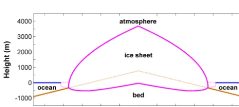
whereV is ice volume,Btot is the total mass accumulation rate on the ice sheet andF is the total ice flux across the grounding line. The mean annual air temperature reduced to sea level and averaged over Antarctica,Ta, and sea level, SL (relative to its 1961–1990 mean), are the only forcings in the original model. As in O5, I take present-dayTa= −18◦C (in the following, present day refers to a 1961–1990 mean). The second term on the right-hand side of Eq. (3) is only con-sidered for a marine ice sheet, that is, forR>rcwherercis the distance from the continent center to where the ice sheet enters the sea. From Eq. (1),rc=(b0−SL)/s, I adopt the O5 approximation of equating the distance from the conti-nent center to the grounding line with the ice sheet radius. Figure 1 shows a cross section of a steady-state solution of the model with standard parameter values and present-day forcing.
The mass balanceBat any height on the ice sheet surface is specified as
B=P forh≥hRand
B=P−β (hR−h)forh < hR, (4)
wherehR(Ta)is the height of the runoff line above which precipitation,P (Ta), is assumed to accumulate as snow and β(P )is a rate of mass balance increase with height. Subli-mation has been disregarded here. The value ofβ depends on a combination of (1) height variations of precipitation and (2) height variations in summertime melting coupled to the atmospheric lapse rate (Oerlemans, 2008). The problem can be easily reformulated in terms of an equilibrium height,he, where the yearly mean mass balance is zero: from Eq. (4)
he=hR−P /β. Likewise, total accumulation and total
ab-lation can be calculated by integratingB over the ice sheet surface above and belowhe, respectively. Results from such a calculation will be presented below. However, integration ofB over the whole surface to obtainBtotis more straight-forward for obtaining problem solutions (O3).
The mass balance part of the problem is closed by choos-ing appropriate expressions forhR,P andβ. For the runoff
line height,
Table 1. Model constants and parameters.
Model and forcing constants
Symbol Description Value
Tf Freezing temperature of seawater −1.8◦C
ρi Ice density 917 kg m−3
ρw Seawater density 1030 kg m−3
ρm Rock density 4000 kg m−3
Ta,0 Present-dayTareduced to sea levela −18◦C
SL0 Present-day sea levela 0 m
To,0 Present-day, high-latitude ocean subsurface temperaturea 0.72◦C
R0 Reference ice sheet radius 1.864×10⁶m
Model parameters
Symbol Description Standard value
b0 Undisturbed bed height at the continent center 775 m
s Slope of the undisturbed bed 6×10⁻⁴
µ Profile parameter for parabolic ice sheet surface 8.7 m0.5 h0 Runoff line height for mean Antarctic temperature reduced to sea level (Ta)equal to 0◦C 1471 m c Proportionality constant for the dependency of runoff line height onTa 95 m (◦C)−1
P0 Annual precipitation forTaequal to 0◦C 0.35 m ice
κ Coefficient for the exponential dependency of precipitation onTa 4×10⁻²(◦C)−1 ν Proportionality constant relating the runoff decrease with height to precipitation 1.2×10⁻²m−0.5yr−0.5 f0 Proportionality constant for ice flow at the grounding line 1.2 m yr−1
γ Power for the relation of ice flow speed to water depth 1/2–17/4b α Partition parameter for effect of ocean subsurface temperature on ice flux 0–1b
aPresent day refers to the mean for the period AD 1961–1990.bRanges over which values are chosen to configure specific model hindcasts.
Figure 1. Cross section of the steady-state DAIS model solution for present-day Antarctic temperature, sea level and ocean subsurface temperature.
whereh0is the runoff line height forTa=0. The values in Table 1 forh0 and the coefficientc were taken from mass balance studies (O4). For precipitation,
P =P0exp(κTa), (6)
whereP0is the (ice equivalent) precipitation at 0◦C and the value of the coefficientκ is chosen assuming a relationship between columnar water content (that increases exponen-tially with temperature) and precipitation (O5). No attempt is made here (nor in O5) to deal with decreasing precipitation
toward the center of the continent. This feature was included in O4 but at the cost of one extra free parameter. For the mass balance gradientβ,
β=P12, (7)
where this relationship and the value of the parameterν in O5 were also based on mass balance observations that reflect in part larger vertical precipitation gradients for greater pre-cipitation (Oerlemans, 2008). Integration ofB over the ice sheet surface yields
Btot=π P R2−πβ(hR−b0+sR)(R2−rR2)
−4πβµ
1 2
5 (R−rR)
5
2+4πβµ
1 2
3 R(R−rR)
3
2, (8)
where rR=R−µ−1(hR−b0+sR)2 is the distance from the continent center to where the runoff line intersects the ice sheet surface. The last three terms in Eq. (8) are consid-ered only whenTa is warm enough for runoff to occur, i.e., forhR> 0. For parameter values of Table 1, this occurs for Ta>−15.48◦C, about 2.5◦C warmer than present day.
the last three terms of Eq. (8) follow from Eq. (2) and the integration of the runoff term in Eq. (4) fromrRtoRby the
use of R
r(R−r)12dr=2
(R−r)52
5 −
R(R−r)32 3
. I also con-firmed the validity of Eq. (8) by comparing with numerical integration of Eq. (4).
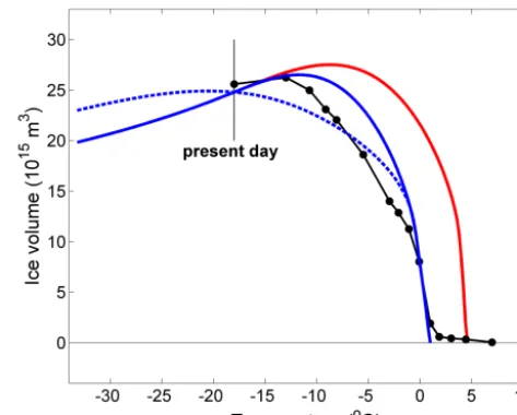
This correction to the original work leads to much reduced runoff and, for the O5 parameter values, an AIS model much less sensitive to climate at warm temperatures. In the cor-rected model, complete Antarctic deglaciation occurs at aTa of about 8◦C higher than in the original model (O4) and about 4◦C higher than in a 3-D thermomechanical model (Fig. 2; Huybrechts, 1993). One possible explanation for this behavior is theβvalue of∼0.001 m ice m−1yr−1for O5 pa-rameter values (calculated at 0◦C). This is a low value for the balance gradient compared to observations, even for dry polar climates (Oerlemans, 2008). To address this I doubled the O5 value ofνfrom 0.006 to 0.012 m−0.5yr−0.5yielding a climate sensitivity at warm temperatures similar to the 3-D model (Fig. 2). 3-Detailed agreement of the idealized 3-DAIS model with the 3-D model cannot be expected since the latter includes a representation of real Antarctic topography. Fur-ther improvements/adjustments of the model runoff formu-lation/calibration will be undertaken in future work. For the present I will concentrate on revised formulations of the other main component of the model: ice flux across the grounding line. This has been the dominant process for ice loss from Antarctica over ice age cycles and will continue to be so in the near future (Pollard and DeConto, 2009).
2.2 Ice flux at the grounding line
In the following, I retain the above O5 mass balance treat-ment (but with the sign corrections) as well as all O5 pa-rameter values except for the revised value ofνand a slight increase of b0 from 760 to 775 m. As in O5, the parame-ter values are chosen to reproduce present-day AIS volume, area, mean surface elevation and mass throughput (Table 1). The ice flux at the grounding line,F, is
F = −(2π Rρw ρi
H )S, (9)
whereρwandρiare water and ice densities,H is the water depth, andSis the ice speed.HandSshould be thought of as some average around the ice sheet periphery over all ice streams. To the grounding line/ice sheet radius approxima-tion menapproxima-tioned above,
H=b0−sR+SL. (10)
The ice flux problem was closed in O5 by assuming that the ice speed is related linearly to the water depth:S=f0H where the value of constant of proportionalityf0was chosen to reproduce present-day AIS throughput (Table 1).
The two recent advances in our understanding of ice flow at the grounding line discussed in the Introduction call for a
Figure 2. Sensitivity of equilibrium solutions of DAIS model ice volume to Antarctic temperature reduced to sea level. Shown are solutions for the original (but corrected) Oerlemans (2005) model (case 1, Table 2) for present-day sea level (SL) and values forν (Table 1) of 0.006 and 0.012 m−0.5yr−0.5(red and blue solid line, respectively) and for a preferred model configuration (case 4, Ta-ble 2) for present-day SL and ocean subsurface temperature (blue dashed line). The black dots are comparable 3-D thermomechanical model solutions (Huybrechts, 1993).
revision of the model ice speed formulation. First, I take ice flux at the grounding line to depend on water depth there raised to a power (Schoof, 2007). Second, I take melting at the base of a marine ice shelf to depend on the temper-ature difference between subsurface tempertemper-ature of the ad-jacent ocean and temperature at the ice shelf base, the lat-ter anchored to the freezing temperature of seawalat-ter. Model-ing studies have yielded a range of such dependencies from linear to quadratic (e.g., Williams et al., 2002; Holland et al., 2008). Below, I am guided mainly by the comprehen-sive, 3-D ocean general circulation model study of Holland et al. (2008), who find a quadratic dependency on this tem-perature difference for a wide range of shelf-slope topogra-phies: they find the melt rate to be proportional to the product of ocean flow speed and ocean temperature beneath the ice shelf, both of which increase linearly with ocean warming. However, I also touch upon results for a model version with a linear dependency on this temperature difference.
With the above motivations I choose to formulate the ice speed as follows:
S=f0 h
(1−α)+α{(To−Tf)/(To,0−Tf)}2 i
Hγ/(b0−sR0)γ−1, (11)
ToandR0is a reference R. In the following, the parameter αwill be taken to vary from 0 to 1 (but values become non-physical toward the upper limit of this range as there will be flow at the grounding line even whenToapproachesTf). The parameterγ will be taken to vary from 1/2 to 17/4. This can be compared to an O5 value of 1 and a value of 15/4 from the results of Schoof (2007; his preferred value forpis 19/4 whereF ∝Hp, therefore from Eqs. (9) and (11),γ=p−1). The value forTo,0was obtained as described in Appendix A, and the value for R0 was taken from the steady-state solu-tion of the O5 model (α=0;γ=1) with present-day forcing (Ta= −18◦C; SL = 0; see below and Table 1). The scaling in Eq. (11) by present-day ocean–ice shelf temperature dif-ference and water depth at the grounding line anchors the present-day ice speed values to the reference solution ice speed for allαandγ values. In the spirit of the original work (O3, O4, O5), the ice speed formulation in Eq. (11) is meant to capture the bulk effect of all individual ice streams and associated embayed ice shelves around the AIS periphery.
The conservation of mass is now dV
dt =Btot(Ta, R)+F (SL, To, R). (12)
The ice sheet is now also forced by ocean subsurface tem-peratureTothat is determined by a combination of local and remote conditions. Model formulation in terms of the inde-pendent variableRis completed by relating ice volume toR, taking into account immediate isostatic adjustment and the effect on this adjustment of the displacement of seawater by ice (O3):
V =π(1+ε1) 8
15µ
1 2R52 −1
3sR 3
−π ε2 2
3s
R3−rc3−b0
R2−rc2
, (13)
where ε1 is ρi(ρm−ρi)−1, ρm is rock density and ε2 is ρw(ρm−ρi)−1. The term multiplied by ε2 in Eq. (13) is only considered for a marine ice sheet (R>rc). Finally, from Eq. (13),
dV
dt =
π (1+ε1) 4
3µ
1 2R
3 2 −sR2
−2π ε2
sR2−b0R dR
dt
−2π ε2
rc2−b0
s rc
d(SL)
dt , (14)
where the terms multiplied by ε2are only considered for a marine ice sheet. Note the sign correction in the last term in curly brackets as well as the extra term at the end of the equa-tion when compared with the original derivaequa-tion in Eq. (13) of O3.
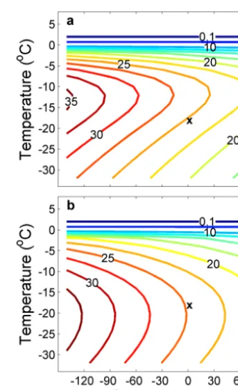
Figure 3. Sensitivity of equilibrium solutions of DAIS model ice volume to Antarctic temperature (Ta)and sea level (SL). Solutions for the original (but corrected) Oerlemans (2005) model and stan-dard parameter values (Table 1; case 1 in Table 2) (a). Solutions for a preferred model configuration (case 4 of Table 2) that also includes sensitivity to high-latitude, ocean subsurface temperature (To)as calculated from Eq. (15) (b). The black crosses mark solu-tions for present-dayTa, SL andTo(Table 1).
2.3 Steady-state solution properties
Figure 3 shows the distribution of AIS ice volume for two different steady-state model solutions as functions of Antarctic temperature and sea level for large ranges ofTa and SL that span past and possible future conditions. The steady-state model ice volume for present-day, yearly mean Antarctic temperature and sea level (Ta= −18◦C, SL = 0) is 24.78×10¹⁵m3(marked by “x” in the figure). Present-day ice volumes for transient model solutions slightly exceed this steady-state value since these solutions are still responding to past temperature and sea level rises. This will be discussed in more detail in Sect. 3.
day, due to increased snowfall and accumulation. Volumes decrease rapidly for still warmer temperatures as melting be-comes important. For very warm temperatures, ice volume isolines become horizontal as the ice sheet recedes out of the ocean, eliminating the dependency on sea level. Ice volume is greater during maximum glacial conditions withTaabout 10◦C colder and SL about 130 m lower than present. Due to the reduced snowfall, increased ice sheet area is needed to balance the ice flux at the grounding line.
Figure 3b shows the steady-state distribution of AIS ice volume for a preferred model configuration from the cali-bration in Sect. 4 (case 4 of Table 2; γ=2, α=0.35 in Eq. 11). This configuration exhibits enhanced ice flux at the grounding line from (1) a higher-order ice flow dependency on water depth there and (2) ice flow increase from ice shelf demise by way of basal melting. In this case, high-latitude, ocean subsurface temperature,To, also comes into play. For the calculations upon which this figure is based, I related
Toto Ta by applying a second-order polynomial fit to val-ues of these temperatures from reconstructions over the past 240 000 years (Appendix A). A best fit with a RMSE of 0.16◦C was found for
To=0.00690(Ta2)+0.439(Ta)+6.39. (15) For example, this yields To= −0.50, 0.72 and 3.32◦C for Ta= −28,−18 and−8◦C, respectively. During colder pe-riods, greater model dependency on sea level leads to less relative dependency of ice volume on temperature (isolines more vertical). Furthermore, ice volume now decreases with warming above present-day values. The increase in ice flux at the grounding line from warmer ocean subsurface tem-peratures, increased basal melting and increased ice shelf demise balances increased snowfall and accumulation from warmer atmospheric temperatures without the need for ice sheet growth. Rather, ice sheet contraction is now needed for equilibrium as temperatures warm.
Figure 4 provides a closer look at ice conservation terms for steady-state solutions of this preferred model configura-tion. The sum of total accumulation (a), total ablation (b) and total ice flux at the grounding line (c) add up to zero for each
Ta–SL combination. As mentioned above, there is a balance between total accumulation and total ice flux forTa of less than−15.5◦C. Likewise, there is a balance between total ac-cumulation and ablation forTaof greater than about−1◦C, at which point the ice sheet has receded out of the ocean. Total accumulation is greatest for Ta of about−5.5◦C, the temperature around which ablation and ice flux are of compa-rable importance. Ablation and ice flux are greatest forTaof about−2 and−13◦C, respectively. All these terms increase as sea level decreases, illustrating the effect of increased ice sheet area and circumference for a lower sea level.
Figure 4. Sensitivity of total equilibrium volume fluxes (1012m3ice yr−1) to Antarctic temperature, sea level and high-latitude, ocean subsurface temperature for the preferred model configuration (case 4 in Table 2). The volume fluxes are (a) accumulation, (b) ablation and (c) ice flux at the grounding line. The black crosses mark solutions for present-dayTa, SL andTo (Table 1).
3 Model calibration and validation
Table 2. Results for specific model configurations.
Present- Remaining 1993–2010 day SL rise to SL rise rate Parameter volume steady-state from AIS
Case Description values (1015m3) (m) (10−3m yr−1)
1 Original Oerlemans model (with corrections)
γ=1,α=0 25.28 1.15 0.15
2 Increased sensitivity of ice flow to sea level
γ=2,α=0 24.97 0.44 0.07
3 Increased sensitivity of ice flow to ocean subsurface temperature
γ=1,α=0.35 25.54 1.75 0.42
4 Increased sensitivity of ice flow to sea level and ocean subsurface temperature
γ=2,α=0.35 25.01 0.53 0.24
5 High sensitivity of ice flow to sea level and ocean subsurface temperature
γ=3.5,α=0.45 24.82 0.09 0.17
interglacial (LIG), the last glacial maximum (LGM) and the mid-Holocene (HOL) at about 6000 BP.
Maximum LIG sea level was considerably higher than present. Recent estimates converge on a range of about 6–9 m above present for this maximum (Kopp et al., 2009; Dutton and Lambeck, 2012). Potential sources for the LIG sea level rise are ocean warming, melting mountain glaciers and ice caps and ice loss from Greenland and Antarctica. DCESS model calculations of ocean warming in Appendix A yield an LIG steric sea level rise of about 0.65 m. Sea level would rise about 0.4 m for melting of all extant mountain glaciers and ice caps (Vaughan et al., 2013); their contribution to LIG sea level rise was probably less than this given that, dur-ing the LIG, global mean temperatures were no more than 2◦C above present day (Fig. A1). Taken together, these two sources can explain an LIG sea level rise of at most 1 m. The Greenland contribution to LIG sea level rise may have been in the range 2.0–2.5 m (Kopp et al., 2009; NEEM, 2013). The sum of these contributions leaves a remaining 2.5–5.5 m to be explained by ice loss from Antarctica. I adopt this range as my LIG constraint.
The AIS was larger during the LGM. Ice sheet and glacial isostatic adjustment (GIA) modeling a decade ago indicated a range of 14–21 m SLE for this size increase (Clark and Mix, 2002; Peltier, 2004; Huybrechts, 2002). However, more recent modeling and GIA studies using local GPS observa-tions show lower values of 8–10 m (Ivins and James, 2005; Whitehouse et al., 2012). This issue needs to be resolved, but for present purposes, I assume the range of 8–17 m SLE for my LGM constraint. By the mid-Holocene, the Northern Hemisphere ice sheets had melted and mean sea level had risen to about 2–3 m below present (Lambeck et al., 2010). Since temperatures had been slightly warmer than present for thousands of years by the mid-Holocene (Marcott et al., 2013), the ocean may have been warmer and less ice than present may have been found in mountain glaciers and ice caps and perhaps also on Greenland (Vinther et al., 2009). These effects would have raised sea level to or slightly above
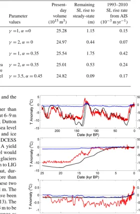
Figure 5. Forcing for DAIS model hindcasts, reconstructed for the period 240 kyr BP to AD 2010 (see Appendix A for details). Shown are the anomalies of Antarctic temperature reduced to sea level (red lines), sea level (black lines) and high-latitude, ocean subsur-face temperature (blue lines), all relative to their present-day values (−18◦C, 0 m and 0.72◦C, respectively). The actual forcings are the anomalies with the addition of these present-day values. The lower two panes are enlarged sections of the full series (top pane). The dashed black line in the top pane shows the original Waelbroeck et al. (2002) sea level reconstruction for the period 140–122 kyr BP (see discussion in Appendix A).
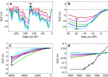
Figure 6. Hindcasts of sea level equivalent (SLE) from changes in AIS ice volume for the five model configurations in Table 2 and for the period 240 kyr BP to AD 2010. The hindcasts are plotted relative to present-day values (means for AD 1961–1990). Shown are results for the original (but corrected) Oerlemans (2005) model (case 1; red lines), for increased sensitivity of ice flow to sea level (case 2, magenta lines), for increased sensitivity of ice flow to ocean subsurface temperature (case 3, green lines), for increased sensitivity of ice flow to sea level and ocean subsurface temperature (case 4, blue lines) and for high sensitivity of ice flow to sea level and ocean subsurface temperature (case 5, cyan lines). Frames (b–d) are enlarged sections of the full hindcasts shown in (a). Paleoreconstruction targets for the last interglacial, the last glacial maximum and the mid-Holocene are shown as vertical bars in (a–c), respectively (see text in Sect. 3 for details). Also shown is reconstructed global mean sea level from 6000 BP to the present (black dashed lines in (c) and (d); see Appendix A for details).
3.1 Hindcasts over the last two glacial cycles
Here, I integrate the time-dependent equations for ice sheet radius, R, from 240 kyr BP to AD 2010 for the forcing in Fig. 5 and for five different model configurations (cases 1–5 in Table 2). The integrations start from the initial condition of
R=R0(1.8636×10⁶m), the radius of the steady-state model solution for present-dayTa, SL andTo. This is a reasonable initial condition for 240 kyr BP during an interglacial period not unlike the present one. Tests with other reasonable ini-tial conditions varying by up to 10 % from the above value produced identical hindcasts from about 220 kyr BP onward. With the use of Eq. (13), ice sheet volume was then calcu-lated and converted to SLE: an SLE of 57 m was taken to correspond to the ice volume of the steady-state model so-lution, 24.78×10¹⁵m3(assuming ice and seawater densities from Table 1 and seawater replacing ice below sea level).
The model hindcast with the original (but corrected) Oer-lemans model (case 1) exhibits a slow, low-amplitude re-sponse to the forcing whereby maximum SLE occurs about 30 kyr after the LIG (red lines in Fig. 6). In this configura-tion the AIS continues to respond significantly at present to sea level rise over the last deglaciation and would continue
to lose mass equivalent to more than 1 m SLE if present-day temperature and sea level were maintained (Table 2). A model hindcast with increased sensitivity of ice flow to sea level rise (case 2) shows a more rapid, higher amplitude response, more in accord with the data constraints (maroon lines in Fig. 6). In this case, the timing but not the ampli-tude of the SLE target at the LIG is achieved. As the model now responds more rapidly to sea level change, much less sea level rise remains from continuing model response to the last deglaciation (Table 2). A model hindcast with increased sen-sitivity of ice flow to ocean subsurface temperature (case 3) shows a still higher amplitude, a good agreement with the SLE target at the LIG but a slow response to the last deglacia-tion (green lines in Fig. 6). Here, almost all the AIS ice loss occurs after 10 kyr BP, the AIS ice volume is too large during the mid-Holocene and there is a remaining sea level rise of nearly 2 m for present-day forcing (Fig. 6; Table 2).
during the LIG was 3.07 m. When rerun using a double-peak structure for LIG sea level rise (Kopp et al., 2009), case 4 yields a very similar maximum with a 500–1000-year extension of high SLE. When rerun using the original Waelbroeck et al. (2002) sea level curve across the LIG (Ap-pendix A; Fig. 5), case 4 yields a slightly lower maximum of 2.31 m. The results of cases 3 and 4 show that the key model feature for simulating an LIG-like ice loss is ocean subsurface warming leading to ice flow acceleration. AIS ice loss during the last deglaciation now occurs mainly after 15 kyr BP and includes a SLE ice loss of less than 1 m at meltwater pulse 1A, forced by ocean subsurface warming and sea level rise across the pulse. This result is consistent with a mainly Northern Hemisphere source of this meltwa-ter event (e.g., Gregoire et al., 2012). The case 4 hindcast is also consistent with a reconstruction of the 220 kyr BP sea level high stand several meters below present-day sea level (Waelbrocke et al., 2002). A model hindcast with higher sen-sitivity of ice flow to sea level rise and to ocean subsurface temperature (case 5) barely meets all three reconstruction tar-gets (cyan lines in Fig. 6). This rapid response of this config-uration to forcing leads to a more rapid AIS shrinking at the last deglaciation. Furthermore, by the Medieval Warm Pe-riod around 1000 years ago, the model AIS has receded to a smaller size than present day.
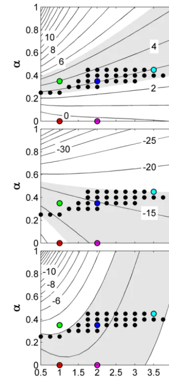
3.2 Comparison with past and present-day estimates Figure 7 shows the results of a more systematic search for the degree to which increased sensitivity of ice flow to sea level rise (as characterized by the parameterγ) and to ocean subsurface temperature (as characterized by the parameter
α) lead to model hindcasts that satisfy all three reconstruc-tion targets. From top to bottom panes, the figure shows iso-lines of Antarctic ice sheet SLE for the last interglacial, the last glacial maximum and the mid-Holocene, respectively, for model hindcasts spanning the ranges of γ and α. The five cases considered in Sect. 3.1 are plotted as colored dots with the coloring scheme as in Fig. 6. The isoline ranges of SLE defined by the reconstruction targets are shaded. Of the 336 hindcasts tested, 29 meet all three reconstruction targets (black dots in the figure). Acceptable values forαare 0.25– 0.45 with the lower values constrained mainly by the LIG get and the higher values mainly constrained by the LGM tar-get. Acceptable values forγ are 1–3.75 and are mainly con-strained by the HOL target. However, most of the acceptable solutions are grouped in theγ range of 1.75–3. These val-ues are somewhat lower than expected from boundary layer theory (3.75; see above), but it should be remembered that they represent some mean of all ice streams around Antarc-tica with varying degrees of ice shelf buttressing. The low-value outliers forγ are coupled to low-value outliers forα.
The above results show some promise for the use of such well-calibrated versions of DAIS in other future applications. After all, the model captured well the timing and amount of
Figure 7. Model hindcasts in specific time slices of sea level equiv-alent (m) from AIS ice volume changes, as functions of model pa-rametersγ and α. These parameters enter in the dependency of ice speed on water depth at the grounding line and on ocean sub-surface temperature, respectively (see Eq. 11). The time slices are (a) the last interglacial period, (b) the last glacial maximum and (c) the mid-Holocene. Reconstruction targets for each time slice are shaded. The black dots mark hindcasts that meet all three paleo-reconstruction targets. The colored dots mark the five hindcasts of Table 2 and Fig. 6 with the Fig. 6 coloring scheme.
0.27±0.11 mm yr−1(Vaughan et al., 2013). Figure 8 shows isolines of this rate for this period as calculated from the same model hindcasts as in Fig. 7. The isoline range de-fined by the recent IPCC estimate is shaded, and the well-calibrated model configurations from Fig. 7 are plotted in Fig. 8. There is a large overlap between the rate of ongoing sea level rise from AIS ice loss for these model combina-tions and the IPCC estimate. For example, the rise for case 4 is 0.24 mm yr−1 (Table 2). Only a few well-calibrated con-figurations with low values of α and high values of γ fall outside the IPCC range.
I also tested a model version identical to the present one except for a linear, rather than quadratic, dependence of basal melting on the temperature difference between the subsur-face temperature of the adjacent ocean and the temperature at the ice shelf base. With this version it was also possible to satisfy all three reconstruction targets but in a much nar-rower parameter space with acceptable values forαof 0.65– 0.7 and forγ of 1.5–2. These few acceptable hindcasts pro-duced rates of ongoing sea level rise from AIS ice loss in the range of 0.24–0.31 mm yr−1, also in good agreement with the recent IPCC estimate.
4 Discussion
Here, I formulated a simple Antarctic ice sheet model by first adopting and making corrections to a published mass balance approach (Oerlemans, 2003, 2004, and 2005) and then by advancing a new treatment of ice flow at the grounding line based on recent advances in our understanding of the controls on this flow. It was then possible to calibrate the resulting DAIS model, as forced by reconstructed Antarctic tempera-ture, sea level and ocean subsurface temperatempera-ture, to simul-taneously satisfy reconstructions of AIS contributions to sea level during the last interglacial, the last glacial maximum and the mid-Holocene. Finally, it was shown that the well-calibrated model hindcasts also reproduced best estimates of the present rate of ongoing sea level rise from AIS ice loss. These results lend some support for the use of the present DAIS model for hindcasts farther back into the past as well as for projections into the future. However, the question arises of how much confidence can be placed in the results of such a simple model. On one hand, well-calibrated simple models have proven useful in many contexts in the past (Shaffer et al., 2009; Meinhausen et al., 2009). On the other hand, there are key questions regarding the AIS that cannot be addressed in detail with the simple DAIS model. Perhaps the most em-blematic of such questions regards the collapse of the West Antarctic Ice Sheet.
Analyses of sea level rise during the last interglacial pe-riod indicate that, during this pepe-riod, the AIS was 2.5–5.5 m SLE smaller than present day (Kopp et al., 2009; Dutton and Lambeck, 2012). The lower end of this estimate coincides with a recent estimate of how much sea level would rise
Figure 8. Model hindcasts of the mean rate of sea level rise (mm yr−1)from ice loss from the AIS for the period AD 1993– 2010 as functions of model parametersγ andα. The present IPCC best estimate for the range of this mean rate is shaded (Vaughan et al., 2013). The black dots mark hindcasts that meet all three paleo-reconstruction targets (from Fig. 7). The colored dots mark the five hindcasts of Table 2 and Fig. 6 with the Fig. 6 coloring scheme.
from the collapse of the present-day West Antarctic Ice Sheet (WAIS) (3.3 m; Bamber et al., 2009). The upper end of this estimate would require some additional contribution from East Antarctica. Basal melting in combination with a high-order dependency of ice flow on grounding thickness facili-tates marine ice sheet instability, such as would likely be ac-tive in a WAIS collapse, but would also increase flow in East Antarctic ice streams (Schoof, 2007; Joughin et al., 2012). Both basal melting and the high-order ice flow dependency were included, albeit schematically, in the DAIS model and made it possible for this simple model to simulate observed AIS ice loss during the LIG when forced by reconstructed ocean subsurface temperatures. Marine ice sheet instability also requires complex bed geometry with the bed sloping downwards in the inland direction. As shown in Fig. 1, the depressed bed of the DAIS model slopes in this manner at the periphery of the ice sheet. However, assumed immediate isostatic adjustment in this highly idealized model immedi-ately restores the initial upward slope. While the model has been calibrated to produce observed LIG ice loss of the size of a WAIS collapse when forced with some realism, it can therefore not be expected to capture detailed timing of a ma-rine ice sheet instability nor high, short-term ice loss rates that would be associated with one. Still, when calibrated with paleo-constraints the model was successful in reproducing the present, short term rate of ice loss from the AIS.
interglacial and a smaller one in the last interglacial, in con-flict with sea level reconstructions (Waelbroeck et al., 2002; Kopp et al., 2009). The well-calibrated hindcasts of the DAIS model presented above (Fig. 6) captured correctly the rela-tive amplitudes of AIS ice loss for these last two interglacials. Perhaps this difference in model behavior can be explained in that the Pollard and DeConto model used deep-sea-coreδ18O and orbital insolation variations to parameterize ocean forc-ing whereas the DAIS model used actual ocean hindcasts, albeit simplified, for this forcing.
I conclude that the DAIS model can be used profitably with care in a number of possible applications. This very fast, semi-analytical model is well suited for very long hindcasts that would not be feasible with 3-D models. One such pos-sibility would be a study of AIS emergence and subsequent evolution over the Cenozoic Era. The DAIS model is also well positioned to be a component in integrated assessment
Appendix A: Forcing reconstructions for the last two glacial cycles
For annual and area mean Antarctic temperature reduced to sea level,Ta, I use temperature anomaly reconstructions ad-justed to a present-day mean temperature of−18◦C (present day refers to a mean of the period AD 1961–1990). For the period 240 000–1500 BP, I adopt temperature anomaly esti-mates from the Dome C ice core (Jouzel et al., 2007) as ref-erenced to 1.2 times the mean global temperature anomaly in the period 1500–500 BP from Mann et al. (2008). The fac-tor 1.2 is an estimated interglacial polar amplification facfac-tor for Antarctica. This referencing led to a small adjustment of
−0.1◦C relative to the published anomalies. For the periods AD 500–1850 and AD 1851–2010, I used the global mean temperature anomaly from Mann et al. (2008) and Morice et al. (2012), respectively, multiplied by 1.2. These two time series have already been referenced to present-day global means. The composite time series forTa was then interpo-lated to 1-year time steps (Fig. 5).
There are no detailed and reliable time series for sea level around Antarctica, so I fall back upon global mean esti-mates. Reconstruction of a specific Antarctic sea level time series would require knowledge of the sources of sea level change over the two glacial cycles and application of non-eustatic corrections for changes in ice mass (e.g., Mitrovica et al., 2001). This is beyond the scope of the present pa-per. For the period 240–21 kyr BP, I adopt SL values from Waelbroeck et al. (2002) but with an adjustment for the last interglacial period (LIG). In this work, the transition of LIG sea level to levels above present day took place at about 124 kyr BP. However, subsequent work put that tran-sition earlier, at 126±1.7 kyr BP (Waelbroeck et al., 2008) and around 130 kyr BP (Dutton and Lambeck, 2012). I ad-just the LIG transition to occur at about 127.5 kyr BP, based on the more recent work, and also adjust the Waelbroeck et al. (2002) curve by a corresponding amount back to the preceding glacial maximum (Fig. 5). For the period 21 000– 7000 BP, I adopt SL values from Clark et al. (2012) that include representations of meltwater events during the last deglaciation. For SL in the period 6000 BP to AD 1869, I use the curve of Lambeck et al. (2010). For 7000–6000 BP, I interpolated linearly between values from the above two sources. Finally, for AD 1870–2010, I adopt SL values of Church and White (2011) adjusted to a present-day value of zero. The composite time series for SL was then interpolated to 1-year time steps (Fig. 5).
High-latitude, ocean subsurface temperature, To, enters the model as a forcing that ultimately modulates ice flow at the grounding line (see Sect. 2). It is a major challenge to construct a realistic time series for To since it will de-pend on some combination of local and remote processes like wind-driven upwelling/downwelling and Atlantic merid-ional overturning circulation strength. Furthermore,To will vary around Antarctica. For this task I take a very simple
Figure A1. Input time series and DCESS model results used in the construction of a high-latitude, ocean subsurface temperature time series for forcing DAIS model hindcasts. Shown are (a) Antarctic and Greenland temperature anomalies (red and blue curves, respec-tively), a target time series for global mean temperature anomaly (short magenta line in upper right-hand corner) and calculated global mean temperature (black line) and (b) low- to middle-latitude and high-latitude zone atmospheric temperatures used to force the DCESS model ocean (red and blue lines, respectively) and calcu-lated high-latitude, ocean subsurface temperature (black line). The thin horizontal black lines in (b) mark present-day values (means for the period 1961–1990) for the respective time series. See Ap-pendix A for details.
vertical mixing in the low-to-middle latitude zone and en-hanced vertical mixing in the high-latitude zone. Parameter values were calibrated by fitting to ocean temperature and carbon 14 observations (Shaffer et al., 2008). The model has only one high-latitude zone, but the poleward extent of that ocean zone matches the equatorward extent of Antarctica. TheToused for the forcing of the DAIS model is then taken to be the average temperature in the depth range 200–800 m of the high-latitude ocean zone (Figs. A1b and 5). The value forTo,0in Table 1 is the meanTofor the period 1961–1990.
For the period 122 400–1500 BP temperature estimates are available from Antarctic and Greenland ice cores (Jouzel et al., 2007; Masson-Delmotte et al., 2006). The GMATA time series for this period is calculated as a mean of the two esti-mates after each is (1) referenced to the 1961–1990 period by referencing to the mean temperature anomaly in the period 1500–500 BP from Mann et al. (2008) and (2) divided by appropriate polar amplification factors. These factors were found to be 3 and 6 for Antarctica and Greenland, respec-tively, by fitting to the Shakun et al. (2012) temperature re-construction for the period 22 000–11 000 BP after referenc-ing that reconstruction to the 1961–1990 period by refer-encing to a common period with the results of Marcott et al. (2013) (Fig. A1a). Lower amplification factors of 1.2 and 2.4, respectively, were adopted for the interglacial part of the 122 400–1500 BP period.
The temperature estimates for the Greenland ice core used above are not available before 122 400 BP. GMATA time se-ries were constructed as above for earlier times but using other estimates for Greenland temperature. For the period 240 000–128 700 BP, this temperature was estimated from
a proxy based on methane data from an Antarctic ice core (Spahni et al., 2005). Global atmospheric methane increases during glacial times are due largely to enhanced emissions from boreal wetlands in response to boreal warming (Fischer et al., 2008). A linear regression of Greenland temperature on Antarctic methane for the period 122 400–150 BP results in the relationT = −51.5+0.0802 [CH4(ppb)]. I also tried several more sophisticated approaches included non-linear regression and applying the simple DCESS model module for atmospheric methane (Shaffer et al., 2008) but found no significant improvement over the simple linear regression in terms of modeled versus observed Greenland temperature for this calibration period.
Code availability
Matlab codes for the DAIS model, the forcing data from 240 kyr BP to the present and instructions for using the model can be downloaded from www.dcess.dk under “DCESS model”.
Acknowledgements. I thank the following people for discus-sions and/or for supplying data: Peter Clark, Robert Kopp, Valerie Masson-Delmotte, Johannes Oerlemans, Mark Siddall, and Claire Waelbroeck. I included the non-linear dependency of ice flow on grounding thickness in response to a comment by Catherine Ritz on an earlier version of the model. This work was supported by Chilean FONDAP 15110009/ICM Nucleus NC120066.
Edited by: D. Goldberg
References
Applegate, P. J., Kirchner, N., Stone, E. J., Keller, K., and Greve, R.: An assessment of key model parametric uncertainties in projec-tions of Greenland Ice Sheet behavior, The Cryosphere, 6, 589– 606, doi:10.5194/tc-6-589-2012, 2012.
Bamber, J. L., Riva, R. E. M., Vermeersen, B. L. A., and LeBrocq, A. M.: Reassessment of the potential sea-level rise from a col-lapse of the West Antarctic Ice Sheet, Science, 324, 901–903, 2009.
Church, J. A. and White, N. J.: Sea-level rise from the late 19th to the early 21st century, Surv. Geophys., 32, 585–602, 2011. Church, J. A., Clark, P. U., Cazenave, A., Gregory, J., Jevrejeva, S.,
Levermann, A., Merrifield, M. A., Milne, G. A., Nerem, R. S., Nunn, P. D., Payne, A. J., Pfeffer, W. T., Stammer, D., and Un-nikrishnan, A. S.: Sea Level Change, in: Climate Change 2013: The Physical Science Basis. Contribution of Working Group I to the Fifth Assessment Report of the Intergovernmental Panel on Climate Change, edited by: Stocker, T. F., Qin, D., Plattner, G.-K., Tignor, M., Allen, S. G.-K., Boschung, J., Nauels, A., Xia, Y., Bex, V., and Midgley, P. M., Cambridge University Press, Cam-bridge, United Kingdom and New York, NY, USA, 2013. Clark, P. U. and Mix, A. C.: Ice sheets and sea level of the Last
Glacial Maximum, Quaternary Sci. Rev., 21, 1–7, 2002. Clark, P. U., Shakun, J. D., Baker, P. A., Bartlein, P. J., Brewr, S.,
Brook, E., Carlson, A. E., Cheng, H., Kaufman, D. S., Liu, Z., Marchitto, T. M., Mix, A. C., Morrill, C., Otto-Bliesner, B. L., Pahnke, K., Russell, J. M., Whitlok, C., Adkins, J. F., Blois, J. L., Clark, J., Colman, S. M., Curry, W. B., Flower, B. P., He, F., Johnson, T. C., Lynch-Stieglitz, J., Markgraf, V., McManus, J., Mitrovica, J. X., Moreno, P. I., and Williams, J. W.: Global climate evolution during the last deglaciation, P. Natl. Acad. Sci. USA, 109, 1134–1142, 2012.
Dutton, A. and Lambeck, K.: Ice volume and sea level during the last interglacial, Science, 337, 216–219, 2012.
Fischer, H., Behrens, M., Bock, M., Richter, U., Schmitt, J., Louler-gue, L., Chappellaz, J., Spahni, R., Blunier, T., Leuenberger, M., and Stocker, T. F.: Changing boreal methane sources and con-stant biomass burning during the last termination, Nature, 452, 864–867, 2008.
Gregoire, L. J., Payne, A. J., and Valdes, P. J.: Deglacial rapid sea level rises caused by ice-sheet saddle collapses, Nature, 487, 219–222, 2012.
Hargreaves, J. C. and Annan, J. D.: Assimilation of paleo-data in a simple Earth system model, Clim. Dynam., 19, 371–381, 2002. Holland, P. R., Jenkins, A., and Holland, D. M.: The response of ice
shelf basal melting to variations of ocean temperature, J. Climate, 21, 2558–2572, 2008.
Huybrechts, P.: The Antarctic ice sheet during the last glacial– interglacial cycle: a three dimensional experiment, Ann. Glaciol., 11, 52–59, 1990.
Huybrechts, P.: Glaciological modelling of the Late Cenozoic East Antarctic ice sheet: stability or dynamism?, Geogr. Ann. A, 75, 221–238, 1993.
Huybrechts, P.: Sea-level changes at the LGM from ice-dynamic re-construction of Greenland and Antarctic ice sheets during glacial cycles, Quaternary Sci. Rev., 21, 203–231, 2002.
Huybrechts, P. and de Wolde, J.: The dynamic response of the Greenland and Antarctic ice sheets to multiple-century climatic warming, J. Climate, 12, 2169–2188, 1999.
Ivins, E. R. and James, T. S.: Antarctic glacial adjustment: a new assessment, Antarct. Sci., 17, 541–553, 2005.
Joughin, I., Alley, R. B., and Holland, D. M.: Ice-sheet response to oceanic forcing, Science, 338, 1172–1176, 2012.
Jouzel, J., Masson-Delmotte, V., Cattani, O., Dreyfus, G., Falourd, S., Hoffmann, G., Minster, B., Nouet, J., Barnola, J. M., Chap-pellaz, J., Fischer, H., Gallet, J. C., Johnsen, S., Leuenberger, M., Loulergue, L., Luethi, D., Oerter, H., Parrenin, F., Raisbeck, G., Raynaud, D., Schilt, A., Schwander, J., Selmo, E., Souchez, R., Spahni, R., Stauffer, B., Steffensen, J. P., Stenni, B., Stocker, T. F., Tison, J. L., Werner, M., and Wolff, E. W.: Orbital and mil-lennial Antarctic climate variability over the past 800,000 years, Science, 317, 793–796, 2007.
Kopp, R. E., Simons, F. J., Mitrovica, J. X., Maloof, A. C., and Oppenheimer, M.: Probabilistic assessment of sea level during the last interglacial stage, Nature, 462, 863–867, 2009.
Lambeck, K., Woodroffe, C. D., Antonioli, F., Anzidei, M., Gehrels, W. R., Laborel, J., and Wright, A. J.: Paleoenvironmental records, geophysical modelling, and reconstruction of sea level trends and variability on centennial and longer timescales, in: Understanding Sea Level Rise and Variability, edited by: Church, J. A., Woodworth, P. L., Aarup, T., and Wilson, W. S., Wiley-Blackwell, Hoboken, NJ, USA, 61–121, 2010.
Mann, M. E., Zhang, Z. H., Hughes, M. K., Bradley, R. S., Miller, S. K., Rutherford, S., and Ni, F. B.: Proxy-based reconstructions of hemispheric and global surface temperature variations over the past two millennia, P. Natl. Acad. Sci. USA, 105, 13252–13257, 2008.
Masson-Delmotte, V., Dreyfus, G., Braconnot, P., Johnsen, S., Jouzel, J., Kageyama, M., Landais, A., Loutre, M.-F., Nouet, J., Parrenin, F., Raynaud, D., Stenni, B., and Tuenter, E.: Past tem-perature reconstructions from deep ice cores: relevance for future climate change, Clim. Past, 2, 145–165, doi:10.5194/cp-2-145-2006, 2006.
Wael-broeck, C.: Abrupt change of Antarctic moisture origin at the end of Termination II, P. Natl. Acad. Sci. USA, 107, 12091–12094, 2010.
Marcott, S. A., Clark, P. U., Padman, L., Klinkhammer, G. P., Springer, S. R., Liu, Z., Otto-Bliesner, B. L., Carlson, A. E., Un-gerer, A. Padman, J., Hee, F., Cheng, J., and Schmittner, A.: Ice-shelf collapse from subsurface warming as a trigger for Heinrich eventsc, P. Natl. Acad. Sci. USA, 108, 13415–13419, 2011. Marcott, S. A., Shakun, J. D., Clark, P. U., and Mix, A. C.: A
recon-struction of regional and global temperature for the past 11,300 years, Science, 339, 1198–1201, 2013.
Meinhausen, M., Meinhausen, N., Hare, W., Raper, S. C. B., Frieler, K., Knutti, R., Frame, D. J., and Allen, M.: Greenhouse-gas emis-sion targets for limiting global warming to 2◦C, Nature, 458, 1158–1162, 2009.
Mitrovica, J. X., Tamisiea, M. E., Davis, J. L., and Milne, G. A.: Recent mass balance of polar ice sheets inferred from patterns of global sea-level change, Nature, 409, 1026–1029, 2001. Morice, C. P., Kennedy, J. J., Rayner, N. A., and Jones, P.
D.: Quantifying uncertainties in global and regional temper-ature change using an ensemble of observational estimates: the HadCRUT4 dataset, J. Geophys. Res., 117, D08101, doi:10.1029/2011JD017187, 2012.
Naish, T., Powell, R., Levy, R., Wilson, G., Scherer, R., Talarico, F., Krissek, L., Niessen, F., Pompilio, M., Wilson, T., Carter, L., DeConto, R., Huybers, P., McKay, R., Pollard, D., Ross, J., Win-ter, D., Barrett, P., Browne, G., Cody, R., Cowan, E., Crampton, J., Dunbar, G., Dunbar, N., Florindo, F., Gebhardt, C., Graham, I., Hannah, M., Hansaraj, D., Harwood, D., Helling, D., Henrys, S., Hinnov, L., Kuhn, G., Kyle, P., Läufer, A., Maffioli, P., Ma-gens, D., Mandernack, K., McIntosh, W., Millan, C., Morin, R., Ohneiser, C., Paulsen, T., Persico, D., Raine, I., Reed, J., Riessel-man, C., Sagnotti, L., Schmitt, D., Sjunneskog, C., Strong, P., Ta-viani, M., Vogel, S., Wilch, T., and Williams, T.: Obliquity-paced Pliocene West Antarctic ice sheet oscillations, Nature, 458, 322– 328, 2009.
NEEM community members: Eemian interglacial reconstructed from a Greenland folded ice core, Nature, 493, 489–494, 2013. Oerlemans, J.: A quasi-analytical ice-sheet model for climate
stud-ies, Nonlinear Proc. Geophys., 10, 441–452, 2003.
Oerlemans, J.: Antarctic ice volume and deep-sea temperature dur-ing the last 50 Myr: a model study, Ann. Glaciol., 39, 13–19, 2004.
Oerlemans, J.: Antarctic ice volume for the last 740 ka calculated with a simple ice sheet model, Antarct. Sci., 17, 281–287, 2005. Oerlemans, J.: Minimal Glacier Models, Utrecht Publishing & Archiving Services, Universiteitsbibliotheek Utrecht, 91 pp., 2008.
Peltier, W. R.: Global glacial isostasy and the surface of the ice-age earth: the ICE-5G (VM2) model and GRACE, Annu. Rev. Earth Planet. Sc., 32, 111–149, 2004.
Pollard, D. and DeConto, R. M.: Hysteresis in Cenozoic Antarctic ice-sheet variations, Global Planet. Change, 45, 9–21, 2005. Pollard, D. and DeConto, R. M.: Modelling West Antarctic ice sheet
growth and collapse through the past five million years, Nature, 458, 329–332, 2009.
Pritchard, H. D., Ligtenberg, S. R. M., Gricker, H. A., Vaughan, D. G., van den Broeke, M. R., and Padman, L.: Antarctic ice-sheet
loss driven by basal melting of ice shelves, Nature, 484, 502–505, 2012.
Rignot, E., Casassa, G., Goginemi, P., Krabill, W., Rivera, A., and Thomas, R.: Accelerated ice discharge from the Antarctic Penin-sula following the collapse of Larsen B ice shelf, Geophys. Res. Lett., 31, L18401, doi:10.1029/2004GL020697, 2004.
Schoof, C.: Ice sheet grounding line dynamics: Steady states, stability, and hysteresis, J. Geophys. Res., 112, F03S28, doi:10.1029/2006JF000664, 2007.
Shaffer, G., Olsen, S. M., and Bjerrum, C. J.: Ocean subsurface warming as a mechanism for coupling Dansgaard-Oeschger cli-mate cycles and ice-rafting events, Geophys. Res. Lett., 31, L24202, doi:10.1029/2004GL020968, 2004.
Shaffer, G., Malskær Olsen, S., and Pepke Pedersen, J. O.: Pre-sentation, calibration and validation of the low-order, DCESS Earth System Model (Version 1), Geosci. Model Dev., 1, 17–51, doi:10.5194/gmd-1-17-2008, 2008.
Shaffer, G., Olsen, S. M., and Pedersen, J. O. P.: Long-term ocean oxygen depletion in response to carbon dioxide emissions from fossil fuels, Nat. Geosci., 2, 105–109, 2009.
Shakun, J. D., Clark, P. U., He, F., Marcott, S. A., Liu, Z., Otto-Bliesner, B., Schmittner, A., and Bard, E.: Global warming pre-ceded by increasing carbon dioxide concentrations during the last deglaciation, Nature, 484, 49–54, 2012.
Shepherd, A., Wingham, D., and Rignot, E.: Warm ocean is erod-ing West Antarctic Ice Sheet, Geophys. Res. Lett., 31, L23402, doi:10.1029/2004GL021106, 2004.
Spahni, R., Chappellaz, J., Stocker, T. F., Loulergue, L., Hausam-mann, G., Kawamura, K., Flückiger, J., Schwander, J., Raynaud, D., Masson-Delmotte, V., and Jouzel, J.: Atmospheric methane and nitrous oxide of the late Pleistocene from Antarctic ice cores, Science, 310, 1317–1321, 2005.
Vaughan, D. G., Comiso, J. C., Allison, I., Carrasco, J., Kaser, G., Kwok, R., Mote, P., Murray, T., Paul, F., Ren, J., Rig-not, E., Solomina, O., Steffen, K., and Zhang, T.: Observations: Cryosphere, in: Climate Change 2013: The Physical Science Ba-sis. Contribution of Working Group I to the Fifth Assessment Re-port of the Intergovernmental Panel on Climate Change, edited by: Stocker, T. F., Qin, D., Plattner, G.-K., Tignor, M., Allen, S. K., Boschung, J., Nauels, A., Xia, Y., Bex, V., and Midgley, P. M., Cambridge University Press, Cambridge, United Kingdom and New York, NY, USA, 2013.
Vinther, B. M., Buchardt, S. L., Clausen, H. B., Dahl-Jensen, D., Johnsen, S. J., Andersen, K. K., Blunier, T., Rasmussen, S. O., Steffensen, J. P., Svensson, A., Fisher, D. A., Koerner, R. M., Raynaud, D., and Lipenkov, V.: Holocene thinning of the Green-land ice sheet, Nature, 461, 385–388, 2009.
Vizcaíno, M., Mikolajewicz, U., Jungclaus, J., and Schurgers, G.: Climate modification by future ice sheet changes and conse-quences for ice sheet mass balance, Clim. Dynam., 34, 301–324, 2010.
Waelbroeck, C., Labeyrie, L., Michel, E., Duplessy, J. C., Mc-Manus, J. F., Lambeck, K., Balbon, E., and Labracherie, M.: Sea-level and deep water temperature changes derived from benthic foraminifera isotopic records, Quaternary Sci. Rev., 21, 295–305, 2002.
the last interglacial sea level high stand to marine and ice core records, Earth Planet. Sc. Lett., 265, 183–195, 2008.
Whitehouse, P. L., Bentley, M. J., and Le Brocq, A. M.: A deglacial model for Antarctica: geological constraints and glaciological modelling as a basis for a new model of Antarctic glacial iso-static adjustment, Quaternary Sci. Rev., 32, 1–24, 2012.