RESEARCH
Bayesian optimization for seed germination
Artyom Nikitin
1*, Ilia Fastovets
1,2, Dmitrii Shadrin
1, Mariia Pukalchik
1and Ivan Oseledets
1Abstract
Background: Efficient seed germination is a crucial task at the beginning of crop cultivation. Although boundaries of environmental parameters that should be maintained are well studied, fine-tuning can significantly improve the efficiency, which is infeasible to be done manually due to the high dimensionality of the parameter space.
Results: Traditionally seed germination is performed in climatic chambers with controlled environmental conditions. In this study, we perform a set of multiple-day seed germination experiments in the controllable environment. We use up to three climatic chambers to adjust humidity, temperature, water supply and apply machine learning algorithm called Bayesian optimization (BO) to find the parameters that improve seed germination. Experimental results show that our approach allows to increase the germination efficiency for different types of seeds compared to the initial expert knowledge-based guess.
Conclusion: Our experiments demonstrated that BO could help to identify the values of the controllable param-eters that increase seed germination efficiency. The proposed methodology is model-free, and we argue that it may be useful for a variety of optimization problems in precision agriculture. Further experimental studies are required to investigate the effectiveness of our approach for different seed cultures and controlled parameters.
Keywords: Seed germination, Machine learning, Gaussian process, Bayesian optimization, Agriculture
© The Author(s) 2019. This article is distributed under the terms of the Creative Commons Attribution 4.0 International License (http://creat iveco mmons .org/licen ses/by/4.0/), which permits unrestricted use, distribution, and reproduction in any medium, provided you give appropriate credit to the original author(s) and the source, provide a link to the Creative Commons license, and indicate if changes were made. The Creative Commons Public Domain Dedication waiver (http://creat iveco mmons .org/ publi cdoma in/zero/1.0/) applies to the data made available in this article, unless otherwise stated.
Introduction
Seed germination has been an interesting subject of study for many years. On the one hand, it is the topic for basic research since many biochemical processes occur dur-ing dormancy and different stages of seed germination. On the other hand, the problem is also of great practi-cal importance: finding the optimal parameters such as substrate material, amount of water supply, air tempera-ture, the proportion of plant growth promoters, etc. is a challenging task. Seed germination comprises many processes, and relationships of factors affecting termina-tion of seed dormancy are very diverse. For example, the aforementioned water and temperature combined with light and nitrate level influence seed germination, how-ever, their effect does depend on the level of dormancy of the seeds [1].
The problem becomes even more challenging when multiple parameters must be considered together, and
specific sets of parameters are supposed to be optimized for each time step. Dynamic models of seed germination have been developed [1–3] to address this issue. These models may be helpful in understanding the underlying processes of seed germination. However, to achieve sat-isfactory optimization results using model-based tech-niques, comprehensive prior knowledge of the problem structure is required [4]. Moreover, particular dynamic models may not be appropriate for the specific condi-tions that these models were not developed for, e.g., dif-ferent plant species, substrates or growth stimulators.
A more adaptive approach, based on machine learning (ML) methods, seems to be promising to tackle this issue. Among those methods the Bayesian optimization (BO) [5, 6] algorithm based on the Gaussian process regres-sion (GPR) is one of the most attractive. It is a black-box optimization algorithm that does not require knowl-edge of the system intrinsics. It is widely used in the ML community for hyperparameter optimization and was even successfully applied in culinary arts [7]. Similarly, an approach based on Genetic Algorithms and GPR has been previously proposed for precision agriculture [8].
Open Access
*Correspondence: [email protected]
1 CDISE, Skolkovo Institute of Science and Technology, Nobelya 3, Moscow, Russia 121205
In this paper, we apply BO to simplified seed germina-tion process in the controllable environment in order to identify the values of the controlled parameters that yield the best germination efficiency. First, we select the num-ber of tunable parameters that we can control during the germination period (several days) with the help of cli-matic chambers, e.g., humidity, temperature, amount of water supply provided and choose the reasonable bounds for these parameters based on the expert knowledge. Then, we iteratively apply BO algorithm, to find the val-ues of parameters that maximize the number of germi-nated seeds. We show that starting with an initial expert knowledge-based guess our approach allows to find such values of parameters that yield solid improvement both when initial germination efficiency is low (first experi-ment) and high (second experiexperi-ment).
Materials and methods
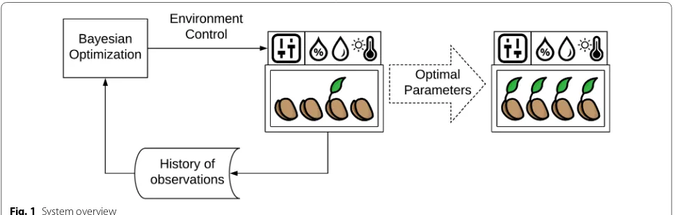
In this section, we describe the methodology and the algorithms used to build our framework. Figure 1 shows a schematic overview of the proposed system.
Seed germination
We conducted two experiments, first, using pea seeds (Pisum sativum L.) and, second, using radish seeds (Raphanus sativa L.) in different settings. Seeds were purchased from Federal Scientific Center of Vegetable (Odintsovo, Russia). The weight of 100 seeds showed an average of 0.751±0.01 g for radish, and of 19.95±1.31 g for pea. All seeds were presterilized in 0.5% of KMnO4 solution for 10 min and then rinsed for several times with deionized water. Three climatic chambers (Binder KBWF 240, KBF 240, KMF 240) allowed to control air temperature ( ±0.1◦C ) and humidity ( ±1% ), which was maintained at 80%. No light sources were used in the chambers during the experiments.
The first experiment was conducted in the form of sequential trials with each trial comprising three concur-rent germination processes and lasting for 72 h (3 days in total). One hundred pea seeds were placed on a dish covered with sterile cheesecloth and put in each of the three climate chambers to germinate. Totally, 7 control-lable parameters were selected: air temperature and the amount of water supplied at 0, 24, 48, 72 and 0, 24, 48 h steps, respectively. The temperature in the chambers was changed smoothly between the selected values during the trials.
During the second experiment, only two climatic cham-bers were used (KBF 240, KMF 240) to set 4 controllable parameters, namely temperatures at 0, 12, 24, 36 h. Seeds were placed in containers of size 21×15.5×0.8 cm with two sections (each accommodating 16 seeds) on the cloth and watered once at the beginning of a trial with a fixed amount of 6 ml. Figure 2 depicts a single container at the beginning (left) and the end (right) of a trial.
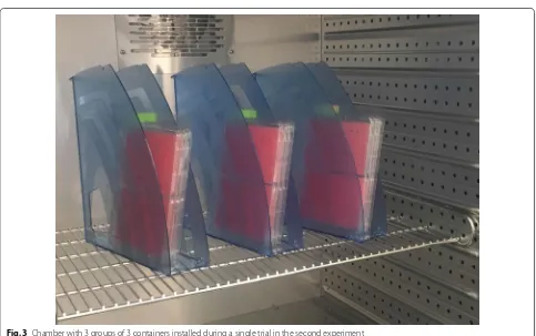
These containers, then, were grouped by 3, giving 96 seeds in a group. Three such groups then were placed almost vertically in each of two climatic chambers with the same controllable parameters set, thus, for each trial giving 6 repetitions with a total amount of seeds equal to 96 in each of them. Figure 3 shows how containers with seeds were installed in the chambers during the second experiment.
After the seeds were germinated, the number of ger-minated and well-gerger-minated seeds were counted in each chamber. In the first experiment, we considered the seeds germinated when only the radicle emerged and could be visibly separated from the seed. If not only radicle but also the hypocotyl emerged and could be visibly separated, the seed was classified as well-germinated. For the second experiment, we considered seeds germinated if radicle emerged and its length is less than 17.5 mm, and well-germinated if it is larger.
Figure 4 shows an example of not germinated (left), germinated (middle) and well-germinated (right) radish seeds according to our methodology.
Bayesian optimization framework
In this section, we describe the Bayesian optimization framework based on the Gaussian process regression that we used in our work.
Fig. 2 Container with radish seeds before germination (left) and after (right)
Fig. 3 Chamber with 3 groups of 3 containers installed during a single trial in the second experiment
where x∈Rd is a vector of d input parameters.
Let consider the GP model with an additive normal noise:
where ǫ∼N(0,σ2). Given the training data X=(x1,. . .,xn)⊺∈Rn×d , y=
y1,. . .,yn ⊺
∈Rn , where
n is the number of available measurements and (·)⊺ denotes the transpose, the predictive distribution at an unobserved point x∗ is given by
where K(X,X) is a matrix of the form
Kij=k(xi,xj),i,j=1,. . .,n. Particular choice of the
kernel function depends on the assumptions about the model and a particular application, however, there exist commonly used kernels, such as Radial basis func-tion (RBF) and Mateŕn that work well in general. Kernel hyperparameters are usually optimized using Maximum Likelihood Estimation (MLE) [10] or its variations.
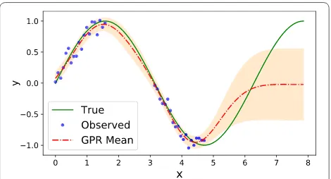
Figure 5 shows an example of GPR using RBF kernel over the sine function with noisy measurements, where predictive variance increases at points with missing measurements. Outside of the interpolation region pre-dictive variance significantly increases with the mean failing to capture the true function trend.
Bayesian optimization
An advantageous property of GPR is that it provides not only the prediction of the value at unobserved points but the complete probabilistic distribution determined by the mean and variance. The general idea behind BO algorithms is to use such distribution to explore param-eter space and select values of x∗ in a way that it will most probably maximize target function f(x) . The common
approach is to select a particular acquisition function that takes parameters of the predictive distribution of the
(1) y(x)=f(x)+ǫ,
f∗∼Nµˆ,σˆ2,
ˆ
µ(x∗)=m(x∗)+K(x∗,X)[K(X,X)+σ2I](y−m(X)),
ˆ
σ2(x∗)=k(x∗,x∗)−K(x∗,X)[K(X,X)+σ2I]−1K(X,x∗),
fitted model as an input and outputs some value which is maximized instead. There exist multiple strategies, for example, using the probability of improvement, expected improvement or integrated expected improvement over the current best value, entropy search or upper confidence bound (UCB) [6]. We have selected the UCB acquisition function in our work as it is easy to evaluate and was shown to be effective in practice. It is expressed using the predictive mean and variance as follows:
Exploration–exploitation trade-off is managed by the parameter κ , where for small κ regions with a high mean (exploitation) and large κ regions with high uncertainty (exploration) are preferred, respectively. We will further omit κ from the arguments of the UCB function where it is assumed fixed.
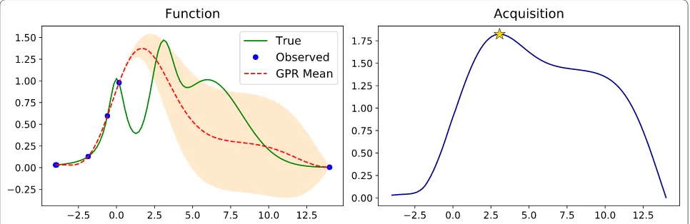
Figure 6 shows the 4th step (with 2 initial data points at the boundaries) of the BO algorithm on an example func-tion with several local maximums using UCB acquisifunc-tion function with the fixed κ=2.
It is critical to note that BO performance is profoundly affected by the dimensionality of the input data due to the exponential growth of the parameter space. It may start to perform poorly when the number of controlled parameters becomes larger than ten [11].
Noise estimation
We defined the target function that we aim to optimize as the sum of averages of germinated and well-germi-nated seeds (see “Seed germination” section). First, let N denote the number of seeds used in the experi-ment. Second, due, to the stochasticity, we model the success of a single seed germination for the fixed values of parameters x as a Bernoulli trial. Then, the probabil-ity that a single seed is germinated equals to p(x)=p , (2)
aUCB(x,κ)= ˆµ(x)+κ· ˆσ (x)
whereas probability that a single seed is well-germi-nated, given that it has germiwell-germi-nated, equals to q(x)=q .
If Ng and Nwg denote the number of germinated and
well-germinated seeds in the experiment, respectively, then, it can be shown that for sufficiently large N (for details, see “Appendix” section) our target function is
where µ=p(1+q) and σ2=p(1+3q)−p2(1+q)2 .
Due to the normality of the obtained distribution, its var-iance can be interpreted as an input-dependent Gaussian noise in the Eq. (1). Therefore, we can simplify hyper-parameter optimization by setting a lower bound of the noise variance with the following value:
Alternatively, for each obtained observation yi a
lower-bound of the noise variance can be estimated as (for details, see “Appendix” section)
in order to incorporate the dependence on the values of observations.
Concurrent experiments
Aforementioned BO formulation assumes that the opti-mization process is sequential, i.e., only a single x∗ is
selected at each step. However, it may be necessary to be able to select several vectors of parameters to explore, e.g., if there are multiple CPU cores for computations or several experimental setups available (climate chambers
y(x)= Ng+Nwg
N ∼ N
µ, 1
Nσ 2
,
(3)
1
N maxp,q σ
2(p,q)= 1
N.
1
N ·yi(2−yi), i=1,. . .,n
in our case). This is referred in the literature as batch set-ting [12, 13] or setting with a delayed feedback [14]. In this work we consider the following approach from [12] to tackle this problem: for each trial comprising the selec-tion of multiple vectors of parameters, we find the maxi-mizer of acquisition function and “observe” the target function using the predictive mean of GPR instead of the real outcome (see Algorithm 1).
Exploration–exploitation control
It may happen when performing exploitation that the algorithm could propose parameters that are very close to the already explored data points, e.g., try 22.001◦C
temperature after 22.000◦C , which yields a change
beyond the controllable precision. In order to cope with this problem and reduce the manual labor of an operator in the selection of κ from Eq. (2) that will give a reason-able exploitation, we propose an additional optimization procedure. First, we formulate the notion of a reasonable exploitation as the following constraint:
(4) min
i=1,...,n
arg maxx aUCB(x,κ)−xi ∞
≥ǫxploit,
where xi is taken from a subset of size s≤n of already
observed points, e.g., one may like to ignore manu-ally initialized data (see “Data preparation” section) and prefer exploration around knowingly good regions. This constraint means that the selected parameters must be at most as ǫxplore far in total form the closest already
observed data point. Algorithm 2 describes the explora-tion–exploitation control procedure.
Experimental evaluation
In this section, we describe the details of our experimen-tal setup and provide the obtained results.
Selecting parameters
We implemented1 our solution with Python 3
program-ming language using the Bayesian optimization library.2
As the covariance function we selected the composition of constant, isotropic Mateŕn (with ν=2.5 , assuming
sufficient smoothness) and white noise kernels with tun-able hyperparameters:
where δij is a Kronecker-delta, α,ρ∈R+ .
Optimiza-tion of the hyperparameters is performed at each step
1
k(xi,xj)=α·Cν(xi/ρ,xj/ρ)+σ2δij
was managed through κ parameter based on the expert knowledge, i.e., at each step, κ was selected in such a way that the algorithm does not purely exploit almost the same parameters or explore knowingly unprofitable regions. Additional control was performed by setting
ǫxploit equal to 0.1◦C and 1 ml and ǫxplore equal to 10◦C
and 100 ml for the temperature and the water supply, respectively. For constrained optimization we have used SciPy [15] library implementation of the Sequential least squares programming (SLSQP) algorithm [16]. Each opti-mization step requires the evaluation of the maximum of acquisition function at several points, which impose computational overhead, however, it can be considered negligible compared to the time-scale of a single trial.
Data preparation
To set up the experiments, we had to consider several issues. First, we had to select the boundaries for the opti-mized parameters: we selected them at 0, 40◦C (in both experiments) and 0, 250 ml (in the first experiment) for the temperature and the water supply, respectively. Sec-ond, as the parameters may have different unit measures, which affects modeling due to isotropy of the selected kernel, we needed to scale them appropriately: we line-arly mapped temperature and water supply values to [0, 1] and [0, 0.5] intervals, respectively, assuming “equiva-lence” of 1◦C and 12.5 ml (during the second
experi-ment, this step was ignored as the only temperature was varied). Finally, we had to add some initial data so that optimization could kick off: we picked all of the possible combinations of 0 and 40 temperatures (in both experi-ments) with 0 water supply (in the first experiment) on each day and assigned the “observed” target function values equal to 0 (totally 24=16 initial points). It can be
considered reasonable as extreme conditions should pro-duce poor results.
Results
First experiment (poorly germinated pea seeds)
For a single germination process, we used N =100
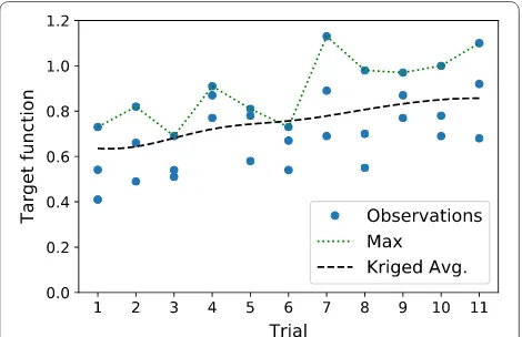
pea seeds and conducted only a single repetition for each selected vector of controlled parameters. The first trial was conducted using the single reference vector of parameters selected with the expert knowledge, which gave the number of germinated seeds equal to 73, and the two vectors selected by the BO algorithm. At the 11th observation the algorithm discovered the param-eters, which yielded 73 germinated seeds with an addi-tional amount of 18 well-germinated. The 20th selected vector of parameters produced as much as 80 germinated and 33 well-germinated seeds, which in total gave a 55% improvement over the initial guess. Subsequent 13 steps didn’t provide any further enhancement.
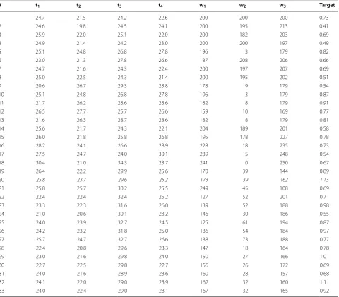
Figure 7 shows the target values obtained during 11 tri-als of the first experiment. Black dashed line denotes the kriged average and shows the trend of improvement in the germination efficiency, whereas the green top dotted line shows the best-observed values for each trial. Table 1 depicts all of the 33 vectors of parameters and respective observed target function values obtained during 11 trials.
Notably, without any prior knowledge of the underlying system, the algorithm was able to learn the values of the controlled parameters that yield sufficient improvement of the germination efficiency. The values of the param-eters that achieved the maximum found target function value of 1.13 at the 20th iteration are listed in italics in Table 1. The identified values can be explained from the physiological point of view. For example, periodically changing temperature may be favorable due to the natu-ral adaptation of seeds to day and night, whereas water
supply identified by the algorithm is in a good agreement with the dynamics of water uptake by seeds, previously described in [17]. According to this study, water uptake by plant seeds is triphasic, comprising a rapid initial absorption, followed by a plateau phase and a further increase due to embryonic axes elongation.
Second experiment (well‑germinated radish seeds)
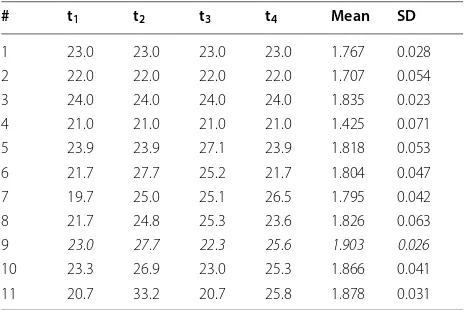
Although the first experiment showed a substantial improvement of germination efficiency in the case of poorly germinated seeds, it could not be that easily observed for well-germinated seeds. Therefore, in the second experiment, we used N=96 radish seeds with 6
repetitions for a single germination trial. The first 4 trials were conducted by setting all of the temperature param-eters as either 21, 22, 23 or 24. At the 9th trial (5th auto-matic step), the algorithm discovered the parameters, which yielded the best average of 10 germinated and 88 well-germinated seeds.
Figure 8 shows the target values obtained during 12 tri-als, where the last trial served as a validation for the best found vector of parameters during the 9th trial. Green dotted line shows the best-observed mean value of the target function, whereas the red dashed line depicts the first expert-knowledge guess-based trial.
Table 2 lists all of the 11 vectors of parameters and the corresponding means and standard deviations of the tar-get function values obtained during 12 trials. The com-plete table containing target function values for every repetition during each trial can be found in Additional file 1.
Although with the initial guess seeds already propa-gated efficiently, the algorithm was able to achieve sub-stantial improvement after the several steps and identify the parameters, which yielded the maximum mean value of 1.903 of the target function with low dispersion.
Conclusions and future work
We applied Bayesian optimization framework to the seed germination process in a controlled environment. Our experiments demonstrated that the proposed method-ology allowed to identify the values of the controllable parameters that increase germination efficiency in dif-ferent settings for difdif-ferent seeds both in the case when initial expert-knowledge based guess yields low and high germination efficiency. The proposed methodology is model-free, and we argue that it may be useful for a vari-ety of optimization problems in intelligent agriculture. Using this approach, we achieved increase in germination efficiency (according to our metrics) from 36.5 to 56.5% by 19 iterations in the first experiment (pea seeds) with low initial germination efficiency, whereas in the second experiment (radish seeds) with high initial germination
efficiency the increase was from 91.8% up to 95.2% by 5 iterations.
We note that selection of the controllable parameters must be made carefully during the preliminary planning. On the one hand, increasing their number allows to per-form better fine-tuning, on the other hand, it makes BO algorithms less efficient and requires more trials to be conducted, which may be both overly time-consuming and equipment demanding.
Combination of the proposed technique with the existing methods of computer vision-based seed counting [18, 19] and seed quality evaluation [20] may decrease manual labor significantly and improve scal-ability. The BO methods definitely could help to reveal optimum chemical parameters of growing mediums or find the environmentally friendly doses of plants biostimulants (humic substances, synthetic hormones, etc.), which effects on plants usually have a nonlinear
Parameters t and w stand for the air temperature in ◦C and the water supply in ml, respectively. The optimal parameters are highlighted in italics
10 25.1 24.8 26.8 27.8 196 3 179 0.87
11 21.7 26.2 28.6 28.6 182 8 179 0.91
12 26.5 27.7 25.7 26.6 159 10 169 0.77
13 21.6 26.3 28.7 28.6 182 8 179 0.81
14 25.6 21.7 24.3 22.1 204 189 201 0.58
15 26.0 21.8 25.8 26.8 195 178 227 0.78
16 28.2 24.1 26.6 28.9 228 18 235 0.73
17 27.5 24.7 24.0 30.1 239 5 248 0.54
18 30.4 21.0 34.3 23.7 241 0 250 0.67
19 26.4 22.2 29.9 25.6 170 39 144 0.89
20 25.8 23.7 29.6 25.2 173 39 162 1.13
21 25.8 25.7 30.2 25.5 249 45 108 0.69
22 22.4 22.4 32.4 25.2 127 52 201 0.7
23 23.3 22.3 31.6 26.0 139 52 188 0.98
24 21.0 20.6 30.1 23.2 146 30 186 0.55
25 24.0 23.9 32.7 24.5 125 61 194 0.87
26 24.2 23.2 31.8 25.0 136 54 184 0.97
27 25.7 24.7 32.7 26.6 138 73 188 0.77
28 22.4 20.8 29.6 23.3 147 18 164 0.78
29 23.0 21.6 29.8 24.0 150 27 166 1.0
30 22.7 22.5 29.8 22.7 156 26 172 0.69
31 24.0 21.6 28.9 23.6 160 28 157 0.68
32 24.1 22.0 29.0 23.9 162 32 160 1.1
dose-effect relationship. Further experimental stud-ies are required to investigate the effectiveness of our approach for this environmental and plants issues. Additionally, we aim to consider partially-controllable environments and apply the proposed method at the next stages of plant growth.
Additional file
Additional file 1. Radish seeds experiment data. The complete list of 11 explored vectors of parameters and target function values obtained dur-ing 12 trials of the second experiment with radish seeds.
Abbreviations
GPR: Gaussian process regression; RBF: radial basis function; MLE: maximum likelihood estimation; BO: Bayesian optimization; UCB: upper confidence bound.
Authors’ contributions
AN: framework design and implementation. IF: initial general idea, preparation and evaluation of the first experiment. DS: preparation and evaluation of the second experiment. MP: consultation, preparation of the second experiment. IO: Initial algorithmic idea, guidance. All authors read and approved the manuscript.
Author details
1 CDISE, Skolkovo Institute of Science and Technology, Nobelya 3, Moscow, Russia 121205. 2 V.V. Dokuchaev Soil Science Institute, Pyzhyovskiy lane 7 bld. 2, Moscow, Russia 119017.
Acknowledgements
This work was supported by the Ministry of Education and Science of the Rus-sian Federation (grant 14.756.31.0001).
Competing interests
The authors declare that they have no competing interests.
Availability of data and materials Data is available on request to the authors.
Consent for publication Not applicable.
Ethics approval and consent to participate Not applicable.
Appendix
Let random variable x∼B(1,p) denote the suc-cess of a seed germination with a probability p and y|x=1∼B(1,q) denote the success of a
well-germina-tion with a probability q given that germination occurred. Using the formula for a full probability:
Then, the distribution of a random variable z=x+y is
with the mean and the variance
Let zi∼pZ, i=1,. . .,N be identically independently distributed random variables. Then, according to the
px,y(x=0,y=0)=1−p px,y(x=1,y=0)=p(1−q) px,y(x=0,y=1)=0 px,y(x=1,y=1)=pq
pz(z=0)=1−p pz(z=1)=p(1−q)
pz(z=2)=pq
(6)
µ=p(1+q),
(7) σ2=p(1+3q)−p2(1+q)2.
Fig. 8 Target function values (blue dots) for each vector of parameters, mean of the initial expert-knowledge guess (red dashed line) and the best found mean for the 9th vector (green dotted line) with around 10 germinated and 88 well-germinated seeds
Table 2 Values of the 11 explored vector of parameters (t1,. . ., t4)T and the corresponding mean and standard deviation values of the target function
Parameters t stand for the air temperature in ◦C . The optimal parameters are
highlighted in italics
# t1 t2 t3 t4 Mean SD
1 23.0 23.0 23.0 23.0 1.767 0.028 2 22.0 22.0 22.0 22.0 1.707 0.054 3 24.0 24.0 24.0 24.0 1.835 0.023 4 21.0 21.0 21.0 21.0 1.425 0.071 5 23.9 23.9 27.1 23.9 1.818 0.053 6 21.7 27.7 25.2 21.7 1.804 0.047 7 19.7 25.0 25.1 26.5 1.795 0.042 8 21.7 24.8 25.3 23.6 1.826 0.063 9 23.0 27.7 22.3 25.6 1.903 0.026
•fast, convenient online submission •
thorough peer review by experienced researchers in your field • rapid publication on acceptance
• support for research data, including large and complex data types •
gold Open Access which fosters wider collaboration and increased citations maximum visibility for your research: over 100M website views per year •
At BMC, research is always in progress.
Learn more biomedcentral.com/submissions
Ready to submit your research? Choose BMC and benefit from: Publisher’s Note
Springer Nature remains neutral with regard to jurisdictional claims in pub-lished maps and institutional affiliations.
Received: 18 July 2018 Accepted: 9 April 2019
References
1. Forcella F, Arnold RLB, Sanchez R, Ghersa CM. Modeling seedling emer-gence. Field Crops Res. 2000;67(2):123–39.
2. Bradford KJ. Water relations in seed germination. Seed Dev Germ. 1995;1(13):351–96.
3. Bello P, Bradford KJ. Single-seed oxygen consumption measurements and population-based threshold models link respiration and germination rates under diverse conditions. Seed Sci Res. 2016;26(3):199–221. 4. Gosavi A. based optimization: an overview. In:
Simulation-based optimization. Operations research/computer science interfaces series, 2nd ed. Boston, MA: Springer; 2015. p. 29–35.
5. Snoek J, Larochelle H, Adams RP. Practical bayesian optimization of machine learning algorithms. In: Proceedings of the 25th international conference on neural information processing systems – NIPS’12, vol. 2. Lake Tahoe, Nevada: Curran Associates Inc.; 2012. p. 2951–2959.
N 1+q N p. 1778–84.
12. Azimi J, Jalali A, Fern XZ. Hybrid batch Bayesian optimization. In: Proceed-ings of the 29th international conference on international conference on machine learning. Madison: Omnipress; 2012. p. 315–22
13. González J, Dai Z, Hennig P, Lawrence N. Batch Bayesian optimization via local penalization. In: Artificial intelligence and statistics; 2016. p. 648–57. 14. Joulani P, Gyorgy A, Szepesvari C. Online learning under delayed
feedback. In: Dasgupta S, McAllester D, editors. Proceedings of the 30th international conference on machine learning proceedings of machine learning research, vol. 28. 2013. Atlanta: PMLR; 2008. p. 1453–61. http:// proce eding s.mlr.press /v28/joula ni13.html.
15. Jones E, Oliphant T, Peterson P, et al. SciPy: open source scientific tools for Python (2001–). http://www.scipy .org/.
16. Kraft D. A software package for sequential quadratic programming. Forschungsbericht- Deutsche Forschungs- und Versuchsanstalt fur Luft- und Raumfahrt; 1988.
17. Bewley JD. Seed germination and dormancy. Plant Cell. 1997;9(7):1055. 18. Ducournau S, Feutry A, Plainchault P, Revollon P, Vigouroux B, Wagner M.
An image acquisition system for automated monitoring of the germina-tion rate of sunflower seeds. Comput Electron Agric. 2004;44(3):189–202. 19. Pouvreau J-B, Gaudin Z, Auger B, Lechat M-M, Gauthier M, Delavault P,
Simier P. A high-throughput seed germination assay for root parasitic plants. Plant Methods. 2013;9(1):32.