High-throughput method for ear phenotyping and kernel weight estimation in maize using ear digital imaging

(1)

Makanza et al. Plant Methods (2018) 14:49

https://doi.org/10.1186/s13007-018-0317-4

METHODOLOGY

High-throughput method for ear

phenotyping and kernel weight estimation

in maize using ear digital imaging

R. Makanza

1

_{, M. Zaman‑Allah}

1*

_{, J. E. Cairns}

1

_{, J. Eyre}

2

_{, J. Burgueño}

4

_{, Ángela Pacheco}

4

_{, C. Diepenbrock}

5

_,

C. Magorokosho

1

_{, A. Tarekegne}

1

_{, M. Olsen}

3

_{and B. M. Prasanna}

3

Abstract

Background: Grain yield, ear and kernel attributes can assist to understand the performance of maize plant under different environmental conditions and can be used in the variety development process to address farmer’s prefer‑ ences. These parameters are however still laborious and expensive to measure.

Results: A low‑cost ear digital imaging method was developed that provides estimates of ear and kernel attributes i.e., ear number and size, kernel number and size as well as kernel weight from photos of ears harvested from field trial plots. The image processing method uses a script that runs in a batch mode on ImageJ; an open source software. Ker‑ nel weight was estimated using the total kernel number derived from the number of kernels visible on the image and the average kernel size. Data showed a good agreement in terms of accuracy and precision between ground truth measurements and data generated through image processing. Broad‑sense heritability of the estimated parameters was in the range or higher than that for measured grain weight. Limitation of the method for kernel weight estima‑ tion is discussed.

Conclusion: The method developed in this work provides an opportunity to significantly reduce the cost of selection in the breeding process, especially for resource constrained crop improvement programs and can be used to learn more about the genetic bases of grain yield determinants.

Keywords: Maize, Ear, Kernel, Phenotyping, Image analysis

(http://creat iveco mmons .org/licen ses/by/4.0/), which permits unrestricted use, distribution, and reproduction in any medium,

provided you give appropriate credit to the original author(s) and the source, provide a link to the Creative Commons license, and indicate if changes were made. The Creative Commons Public Domain Dedication waiver (http://creat iveco mmons .org/

publi cdoma in/zero/1.0/) applies to the data made available in this article, unless otherwise stated.

Background

In maize, yield is a function of interdependent charac-teristics of ears and kernels [1]. A well-developed maize ear may have close to a thousand kernels [2]. The num-ber of kernels per ear is a function of ear width (ker-nels per row) and kernel rows per ear. Many stresses can affect row number and kernels per row, as well as kernel size/weight. Cairns et al. [3] reported that under drought conditions, yield loss in both hybrids and inbreds was largely associated with a highly signifi-cant decrease in the number of kernels per unit of ear area. Plant water deficit at flowering has been shown to

negatively affect kernel number [4] and deficiencies in N supply usually decrease grain yield by lowering ker-nel number per plant [5, 6] as a result of less synchro-nous pollination [7], and/or greater kernel abortion [8]. This indicates that these ear and kernel features can be used to assess the tolerance of a variety to a stressful condition. From a breeding perspective, studies have found that yield components tend to display greater heritability than overall yield [9, 10]; making it possi-ble to select for these traits separately and then com-bine the responsible genetic loci to develop a genotype with superior performance or develop a selection index through traits combinations [11]. According to Miller et al. [1], if maize ears, and kernels attributes could be automatically measured with greater objectivity and precision, more could be learned about the genetic

Open Access

Plant Methods

*Correspondence: [email protected]

1_{International Maize and Wheat Improvement Center (CIMMYT), PO Box}

MP163, Harare, Zimbabwe

(2)

bases of yield components and how to improve them using current and future maize genetic resources.

There are few methods that allow the extraction of ear and kernel features through image processing. A method of evaluating one or more kernels of an ear of maize using digital imagery was patented by Pioneer (Hi-Bred International, inc., Iowa) in 2009 [12]. The method enables to extract kernel count, kernel size distribution, proportion of kernels aborted and other information using image processing algorithms that include, without limitation, filtering, watershedding, thresholding, edge finding, edge enhancement, color selection and spectral filtering. Zhao et al. [13] have proposed a method that provides kernel counts from ear photos, with the assumption that a maize ear has double the number of rows and kernels than can be vis-ible on a photo. More recently, Liang et al. [14], have developed a method that scores maize kernel traits based on line-scan imaging. The method provides 12 maize kernel traits through image processing under controlled lighting conditions. In addition, Miller et al. [1] have proposed three custom algorithms designed to compute kernel features automatically from digital images acquired by a low cost platform. One algorithm determines the average space each kernel occupies along the cob axis using a sliding-window Fourier transform analysis of image intensity features. The sec-ond one counts individual kernels removed from ears, including those in clusters. The third one measures each kernel’s major and minor axis. The main limitation of these methods is that they often rely on systems like a scanner that have controlled lighting conditions and fixed image background. In addition, they do not pro-vide a comprehensive data set from a single image of unthreshed ears i.e. ear count, ear and kernel features simultaneously in an automated manner.

Although there are harvesting equipments that auto-matically measure grain yield on a plot level, yield com-ponent traits such as ear and kernel dimensions are usually measured by hand [15–17]. In addition, this kind of equipment is quite expensive to buy and maintain, therefore not affordable for most breeding programs, especially in sub-Saharan Africa. Digital imaging pro-vides a rapid and low-cost option to collect a large num-ber of ear related traits and has the potential to improve our ability to evaluate yield potential in a breeding pro-gram and ultimately help characterize maize lines and advance our understanding of the genetic mechanisms controlling the fundamental yield components [1].

This work reports a simple, high-throughput and robust method for extracting yield components (ear and kernel attributes) from harvested maize ears using ear digital imaging (EDI).

Materials and methods

Germplasm and experiments

The study was conducted at CIMMYT research station (17°43′37.21′′ S, 31°01′00.60′′ E, and altitude 1489 m above sea level) in Harare, Zimbabwe.

Development of kernel count and weight models To

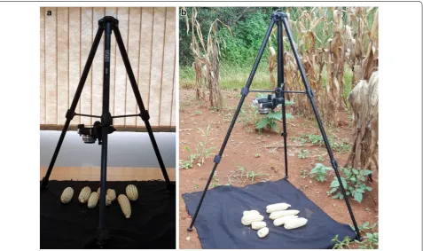
develop these models, one trial composed of 10 hybrids was planted in two replicates on 3 December 2015 using an alpha lattice design. Each hybrid was represented by 2-row plots that were 4 m long with inter-row spacing of 0.75 m and in-row spacing of 0.25 m (Fig. 1). Each plot had approximately 34 plants. After physiological matu-rity, the ears were collected from each plot separately and dried to approximately 10–12% kernel moisture content.

Validation of the EDI method for ear and kernel count and size The validation was performed using one trial composed of 50 hybrids that were planted in three repli-cates on 15 December 2016 using an alpha lattice design with a total of 150 plots. The plots specifications were the same as described above. At harvest, the ears were selected from different ear sizes so as to cover as much as possible a large range of sizes.

Validation of kernel weight model and heritability of traits To validate the kernel weight model and assess the broad-sense heritability of ear traits generated through EDI, a total of six breeding trials were planted on 15 December 2016 using an alpha lattice design. They were composed of advanced elite and pre-commercial sub-tropical maize hybrids which were separated into three maturity groups; early, intermediate and late based on the number of days to flowering. Four of the trials had 50 hybrids each and the remaining two were composed of 55 hybrids each. Trials were all under low nitrogen stress. The plot specifications were the same as described above. Therefore, each trial with 50 hybrids had a total of 150 plots while those with 55 hybrids had 165 plots. For each plot, the ears were collected from all plants after physi-ological maturity.

Photo acquisition

(3)

Page 3 of 13 Makanza et al. Plant Methods (2018) 14:49

Fig. 1 Overall view of the experimental setup and single plot details

(4)

validation were also taken per plot under field conditions using a similar set up (Fig. 2b).

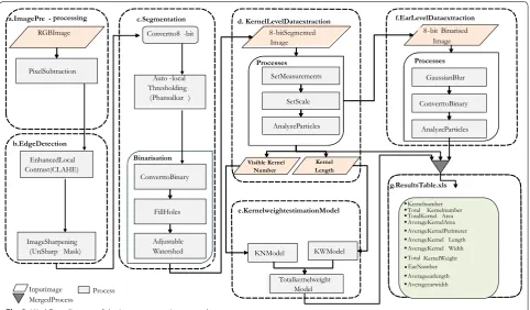
Image processing

Image analysis was conducted in imageJ [18], an open source software. Figure 3 shows a series of steps that were performed to segment and extract yield components parameters (i.e. ear and kernel attributes). These steps were performed using ImageJ plugins. An image pre-pro-cessing step was firstly carried out to distinctively sepa-rate the foreground (ears) from the background objects. Although there were many different ways to achieve this, a single image pixel subtraction method was used, which deducts a constant pixel value from an image. The pixel subtraction threshold was set to 100 based on tests car-ried out with 20 selected images contrasting for illumi-nation gradient of the background to prevent foreground information loss. As a result, an image with an uniformly darker background intensity was produced (Fig. 4b). In this way, background pixels with same color intensi-ties as kernels were suppressed minimizing possibility of significant noise during segmentation. Kernels are separated from one another by lines in between them over narrow colour gradients with fuzzy boundaries. The extent of boundary fuzziness and other surface artefacts of different nature could result in distortion of kernel edges owing to segmentation problems. Segmentation of

kernels is primarily based on the clear definition of these edges whilst minimizing the effects of artefacts on their surfaces. Consequently, contrast limited adaptive histo-gram equalization (CLAHE) method was implemented to enhance the kernel edges whilst suppressing surface noise [19]. Unlike ordinary adaptive histogram equaliza-tion (AHE), which maps a narrow range of input intensity values on a wider range of output intensities values lead-ing to over-enhancement of noise, with CLAHE, a maxi-mum count of intensities can be enforced to limit the enhancement thereby reducing noise [19]. Whilst there is no enhancement at intensity value of 1, an increase in intensity levels subsequently increases enhancement. CLAHE is a well-known block-based processing, and it can overcome the over amplification of noise problem in the homogeneous region of image with standard histo-gram equalization.

The CLAHE plugin has three parameters. (i) Block size, which defines the size of the local region around a pixel for which the histogram is equalized, was set to 29, (ii) the number of histogram bins used for his-togram equalization set to 256. The implementation internally works with byte resolution, so values larger than 256 are not meaningful. Then the maximum slope, which limits the contrast stretch in the intensity trans-fer function, was set to 5 (the value 1 will not result in any change in the original image). Enhanced edges

rne rne

RGB Image

Pixel Subtraction

Enhanced Local Contrast (CLAHE)

b. Edge Detection

Auto -local Thresholding (Phansalkar )

a. Image Pre - processing

Image Sharpening (UnSharp Mask)

c. Segmentation

Convert to 8 -bit

d. Kernel Level Data extraction

8-bit Segmented Image

Kernel Length

rne

KN Model

Visible Kernel Number

KW Model Total kernel weight

Model

e. Kernel weight estimation Model Kernel numberTotal Kernel number Total Kernel Area Average Kernel Area Average Kernel Perimeter Average Kernel Length Average Kernel Width Total Kernel Weight Ear Number Average ear length Average ear width

8-bit Binarised Image

Gaussian Blur Convert to Binary

Analyze Particles

f. Ear Level Data extraction

Processes

Convert to Binary

Fill Holes Adjustable Watershed

Set Measurements Set Scale Analyze Particles

Binarisation

Processes

g. Results Table.xls

Input image Process Merged Process

(5)

were then sharpened to increase their intensity levels using the unsharp mask method with a radius of 5 and a mask set to 0.70. The image was then converted to 8-bit format.

Suppression of artefacts of low contrast was not com-pletely dealt with at edge detection. A local threshold method by Phansalskar [20], a modification of Sauvola’s [21] method was used, which proved to be more effective in cytological images of low contrast. The threshold T(x, y) is calculated according to Eq. (1), where m(x, y) is the mean and s(x, y) standard deviation of pixel intensities, R is the dynamic range of standard deviation which is equal to 0.5 for normalized images, k constant in the range (0.2–0.5), q and p are Phansalkar’s exponential constants.

In the Phansalkar’s plugin, k and r are referred as parameters 1 and 2 respectively. They were kept to default values k = 0.25 and r = 0.5 which worked very well across ear types.

The radius of the local domain over which the thresh-old will be computed was set to 15. The white object on

(1)

T

x,y

=m

x,y

1+pe−q.m(x,y)₊_k

s

x,y

R

−1

black background option was selected to set to white the pixels with values above the threshold value (otherwise, it sets to white the values less or equal to the threshold).

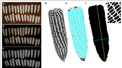
The images were then binarized with filling of holes to achieve solid kernel shapes which prevents splitting dur-ing the watershed step (Fig. 4c, d). An adjustable water-shed plugin which provides flexibility through a wide range of tolerance levels to suit different kernel edge smoothness and shapes was applied with a tolerance of 3. The tolerance value determines the difference of radius between the smaller of the largest inscribed circles and a circle inscribed at the neck between the particles. The higher this value, the fewer segmentation lines and low values tend to produce false segmentations, caused by the pixel quantization. In this way kernel segmentation was successfully performed with minimum errors. The com-putational workflow is able to estimate yield components parameters (number of ears, size, kernel number and size) from approximately six images or plots per minute.

Kernel counts and attributes

The segmented images were then used for particles anal-ysis after setting the minimum and maximum pixel area size (0.03–1.0 pixels2_{) to exclude anything that is not an}

(6)

values were set within the interval 0.15–1.00 to help excluding unwanted objects with a value of 1.0 indicating a perfect circle. Circularity is a shape descriptor (https :// image j.nih.gov/ij/docs/guide /146-30.html). As the value approaches 0.0, it indicates an increasingly elongated shape. Kernel length and width are referred here as the longest distance between two points along the major and minor axis on a single kernel on the ear, respectively (Fig. 4g). In addition, the total kernel area, as the sum of all individual kernel areas on the image, and the average kernel area were generated using particle analysis. The average perimeter represents the average length of the outside boundary of all kernels that are on the analyzed image. Qualitative attribute like kernel color and ear tex-ture were not included as they can be identified easily from visual observation.

Ear count and attributes

For the ear count, kernels were filtered out via a Gaussian blur method. This filter uses convolution with a Gauss-ian function for smoothing (https ://image j.nih.gov/ij/ docs/guide /146-29.html#sub:Gauss ian-Blur). The param-eter sigma was set to 10. Sigma is the radius of decay to exp(−0.5), (≈ 61%), i.e., the standard deviation (σ) of the Gaussian. This was followed by a binarization step with filling up of holes to avoid splitting ears during the watershed process that was performed with a tolerance of 40 (Fig. 4f). The number of ears was then computed from particles analysis after setting the minimum and maximum pixel area size (> 10 pixels2_{) to exclude}

any-thing that is not an object of interest in the image (https ://image j.nih.gov/ij/docs/guide /146-30.html#toc-Subse ction -30.2). Ear length and width are referred here as the longest distance between two points along the major and minor axis on a single ear, respectively (Fig. 4f).

Kernel count and kernel weight models

The development of a model to estimate the total number of kernels from photos of dehusked ears was done in two steps:

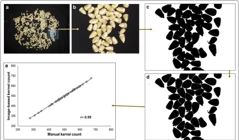
• To compare image-based kernel counting method with the manual kernel count, 50 randomly selected ears were threshed and their kernels put separately in paper bags. The kernels of each ear were first counted manually and then spread on a dark background and photographed using a camera (same set up as above). These images had numerous kernels in clusters (Fig. 5a, b). They were processed using imageJ plugins i.e. transformation into 8-bit, binarization, adjustable watershed with a tolerance of 3 and particle analysis (Fig. 5c, d). The correlation between the two meth-ods was r = 0.99 (Fig. 5e). Therefore, the image-based

kernel counting was considered as equivalent to the manual kernel counting method for kernels removed from ears.

• To estimate the total number of kernel on a given ear from the number of kernels that are visible on a photo of the same ear, 340 ears were photographed individually using the same set up described before. The same ears were then threshed to remove their kernels which were put separately in paper bags and counted using the image-based kernel counting method describe above.

A linear regression model for predicting total ker-nel number on an individual ears was developed from the number of kernels that are visible on the image (kn) (Eq. 2, r = 0.98***). The Pearson’s correlation coefficient r, was used to assess the relationship between estimated and measured kernel parameters.

where kn is the number of kernels visible on the photo. The kernel weight model was developed using a linear regression model between average kernel length ( kl ) and the average kernel weight (total kernel weight divided by the total number of kernels) measured manually using a digital balance (Mettler Toledo), at a precision of 0.01 g. Kernel weight was measured at a moisture content rang-ing from 11 to 13%. This was done usrang-ing 200 ears with contrasting kernel size. The average kernel length was extracted from the visible part of the segmented ear. kl was plotted against the average measured kernel weight for each individual ear measured manually to develop a model that translates kernel length into kernel weight (Fig. 6a). The model was then tested and exhibited a quite accurate estimation of the kernel weight (Fig. 6b).

where kl is the average kernel length.

Kernel weight estimation

Given that Eq. 2 provides the total kernel number and Eq. 3 the average kernel weight, the total kernel weight (Eq. 4) was computed as the product of these two equations:

The estimated total kernel weight was validated using plot level (2 rows plants, 34 plants) images acquired under field conditions from six different breeding trials.

(2)

Total kernel number=2.4051∗kn−6.7334

(3)

Average kernel weight

g

=

kl∗0.7435

−0.155

(4)

Total Kernel Weight

g

=(2.4051∗kn−6.7334)

(7)

Fig. 5 Example of image‑based kernel count: a original image, b image section with many kernels in clusters, c transformation into 8‑bit and binarization, d after adjustable watershed and e correlation between image‑based kernel count and manual kernel count for 50 randomly selected ears

0.2 0.25 0.3 0.35 0.4 0.45 0.5

0.2 0.3 0.4 0.5

Measured kernel weight (g) r= 0.94

RMSE=0.046 CCC=0.92

Estimated

Kernel

weight (g

)

y = 0.7435x - 0.1558 r = 0.92

0.2 0.25 0.3 0.35 0.4 0.45 0.5

0.5 0.6 0.7 0.8 0.9

Kernel weight (g

)

Kernel length (cm)

a b

(8)

Data reliability test

Lin’s concordance correlation coefficient (CCC = ρc) [22]

was used to test the data reliability.

where µ1= E(Y1), µ2= E(Y2), E = expected value,

σ₁2₌ Var(Y₁), σ₂2₌ Var(Y₂), and σ₁₂₌ Cov(Y₁, Y₂) ₌ σ₁ σ₂ ρ, Cb= 2 σ1σ2/[σ12+σ22+(µ1−µ1)2].

(ρc) measures both precision (ρ) and accuracy (Cb).

(ρ) = Pearson’s correlation coefficient, a measure of how close the data are about the line of best fit.

(Cb) = Bias correction factor, a measure of how far

a line of best fit (i.e. the line of perfect concordance) is from a 45 degree angle through the origin.

Lin’s coefficient is 1 when all the points lie exactly on the 45-degree line drawn through the origin and dimin-ishes as the points depart from this line and as the line of best fit departs from the 45-degree line [23].

Broad‑sense heritability

The broad-sense heritability is the ratio of total genetic variance (VG) to total phenotypic variance (VP).

Broad-sense heritabilities were computed using Meta-R (multi environment trial analysis with Meta-R for windows) version 6.01 01 [24] and compared among traits for sev-eral field experiments.

Linear models were implemented using REML (restricted maximum likelihood) to calculate BLUEs (best linear unbiased estimations) and BLUPs (best lin-ear unbiased predictions) and estimate the variance components.

The broad-sense heritability of a given trait at an indi-vidual environment was calculated as:

where σg2 and σe2 are the genotype and error variance components, respectively, and nreps is the number of replicates.

The genetic correlation between traits was calculated as:

(5)

ρ_c= 2σ12

σ₁2+σ₂2+(µ1−µ1)2

=ρCb

(6)

H2= VG/VP

(7) H2=

σ_g2

σ2

g +σe2/nreps

(8) ρg =

σ_g₍_jj′₎

σ_g₍_j_)σ_g₍_j′₎

where σ_g₍_jj′₎ is the arithmetic mean of all pairwise

geno-typic covariances between traits j and j′, and σ_g₍_j_)σ_g₍_j′₎

is the arithmetic average of all pairwise geometric means among the genotypic variance components of the traits.

The relationships between the image variables and ref-erence measurements were tested for significant correla-tion using the Pearson correlacorrela-tion coefficient.

Results

Kernel count and ear attributes

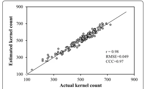
The kernel count model was tested using 180 ears selected over a range of ear sizes from 150 plots as described in the methodology section. Data showed a linear correlation (r = 0.98, p < 0.001) between the estimated kernel count from intact ears using the model and the actual count of detached kernels (Fig. 7). The same ears used for kernel count vali-dation were also used to compare manual measurements of ear length and width with those generated through the image processing method. Data presented a linear correla-tion (r > 0.98, p < 0.001) between the two methods for both traits (Fig. 8 a,b). A similar result was recorded for ear count that is much easier to do (data not shown).

Kernel weight estimation

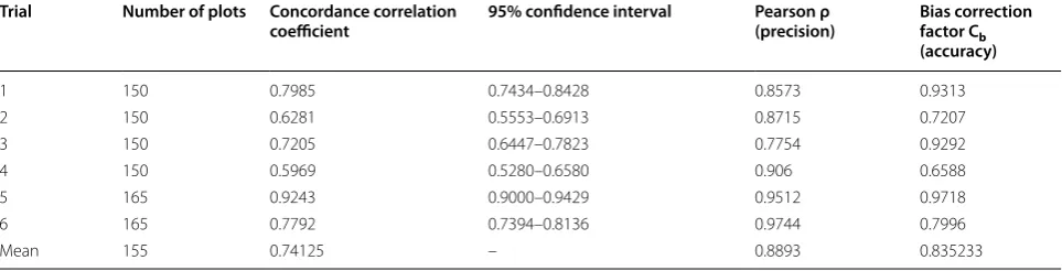
To validate the kernel weight estimation method, data were collected from six field trial (as described in the methodology). Measured kernel weight was compared with estimated kernel weight using the Lin’s concordance test. Results show that the values of the concordance cor-relation coefficient are all above 0.70 except for trials 2 and 4; with an average of 0.74 (Table 1). Average values of precision and accuracy were 0.88 and 0.83, respectively. This indicates that overall, the estimated kernel weight is in relatively good agreement with the measured kernel weight.

100 300 500 700 900

Actual kernel count

r = 0.98 RMSE=0.049 CCC=0.97

Estimated

kernel coun

t

(9)

Heritability of kernel and ear attributes

Broad-sense heritability for measured grain yield aver-aged 0.44 across all trials, similar to that of estimated (Table 2) total kernel weight and total ear area, but signif-icantly lower if compared to the heritability of kernel size (average length and width, average area and perimeter) and to a lesser extent the total kernel number (Table 2). The number of ears per plot and the average ear length had higher heritability than measured grain yield, which is not the case of average ear width.

Discussion

Maize grain yield can be described as a function of the number of harvestable kernels and their individual weight. From these two yield determinants, kernel num-ber usually explains most variation [25] and is strongly related to ear size. Several studies have reported that kernel weight is a highly heritable trait [26, 27], varying markedly among genotypes [28] and largely influenced by genotype × environment interactions. Maize kernel

weight is associated with the duration of the grain-filling period, the rate of kernel biomass accumulation, the rate of kernel desiccation and the moisture concentration at physiological maturity [29]. All these traits had large phe-notypic variation and significant response to the interac-tion between genotype and environment [30]. Although very important, kernel traits are not easy to measure rapidly and accurately, partly due to the need for ear threshing before they can be measured. Kernel count can be done manually by counting the number of rows and multiplying that by the number of kernels in one length of the ear. Regarding ear number and size, the manual methods of data collection include measuring directly the dimensions of an individual ear or kernel with cali-pers [17]. These manual measurements of yield compo-nents have been useful and were, for example, used for a divergent selection study of the relationship between ear length and yield [31]. The problem with these meth-ods is the lack of consistency that is inherent to the way the data is collected (dependent on the training and

5

10

15

20

25

30

35

5

15

25

35 Measured ear length (cm)

Estim

ated ear length

(c

m)

r =0.99 RMSE=0.03 CCC=0.97

3

4

5

6

7

3

4

5

6

7 Measured ear width (cm)

Estim

ated ear width (c

m)

r =0.97 RMSE=0.035 CCC=0.945 b

a

Fig. 8 Relationship between measured and estimated ear a length and b width, (CCC = concordance correlation coefficient; RMSE = root‑mean‑square error and r = ρ = Pearson’s correlation coefficient)

Table 1 Lin’s concordance correlation coefficient between measured and estimated kernel weight. Data are from six hybrid trials conducted under low soil nitrogen conditions at Harare, Zimbabwe, during the season 2016–2017

Trial Number of plots Concordance correlation

coefficient 95% confidence interval Pearson ρ (precision) Bias correction factor C_b (accuracy)

1 150 0.7985 0.7434–0.8428 0.8573 0.9313

2 150 0.6281 0.5553–0.6913 0.8715 0.7207

3 150 0.7205 0.6447–0.7823 0.7754 0.9292

4 150 0.5969 0.5280–0.6580 0.906 0.6588

5 165 0.9243 0.9000–0.9429 0.9512 0.9718

6 165 0.7792 0.7394–0.8136 0.9744 0.7996

(10)

Table

2

Br

oad-sense heritabilities (

H

2) and

means f

or

gr

ain yield and

k ernel/ear a ttribut es estima ted thr ough imaging f or six maiz

e trials with

thr ee r eplic at es ev alua ted under lo

w soil nitr

ogen a t Har ar e, Zimbab w e EHY B ear ly h ybr id tr ial , IHY B in ter media te h ybr id tr ial , LHY B la te h ybr id tr ial Trial Number of M easur ed Gr ain yield(Mg ha − 1) Br oad ‑sense heritabilit y (H 2) K ernel a ttribut es Ear a ttribut es En tries (h ybrids) Year V

isible _Kernel _Number

M

ean

width (cm)

M

ean

length (cm)

Total ar ea (cm 2) M ean ar ea (cm) M ean perimet er (cm)

Total Number per

plot

Total Weigh

t

(g

plot

−

1)

Number per

plot

M

ean

length (cm)

(11)

appreciations of the staff devoted to that task), the time and associated cost, which makes them mostly suit-able for very small trials. From a preliminary assessment (data not shown), the proposed EDI method can be twice (example: ear count) to five-fold (example: ear dimen-sions) or more, faster than the manual methods depend-ing on the targeted measurement. The manual methods are labor intensive, which makes them costly as com-pared to the EDI method. The difference in terms of cost would depend on the location/country because of varia-tions in the cost of labor. Yield component studies as well as selection for crop improvement could take advantage of automated measurements that are more consistent, fast and low-cost. For example, Takanari et al. [32] and Moore et al. [33] mapped quantitative trait loci (QTL) in rice and Arabidopsis, respectively using image-derived size and shape phenotypes.

Miller et al. [1] have proposed an imaging method of kernel counting based on individual kernel area. The method estimates also kernel size (width and depth) but only on detached kernels. While this method is quite precise, it requires that the kernels are removed from the ears; which may not be convenient especially when dealing with a large number of ears. Similarly, Liang et al. [14], have also developed a method that scores maize kernel traits based on line-scan imaging that cannot be suitable for assessment in the field in terms of time and cost. The advantage of the proposed EDI method it that it generates ear and kernel attributes data from images of intact ears. The approach is to some extent similar to that of Grift et al. [34] who have developed a machine vision-based method to count maize kernels on the ear within a quasi-cylindrical mid-section and ear maps. While their method is, to a large extent, interesting; the imag-ing is done in a soft box fitted with a light reflector and high-quality diffused lighting scene. The limitation of this type of imaging set up is the throughput. Regarding ear size, the EDI method showed a good agreement between manually measured ear dimensions and the results of automated image processing (Fig. 8). Similar results were reported by Miller et al. [1]. The main difference between the two methods is that the one proposed by Miller et al. [1] uses flatbed document scanners to acquire ear images whereas the EDI method makes use of RGB camera. In addition, while the flatbed scanner gives the advantage of controlling lighting conditions; the logistics associated with using it in the field (i.e. need of a computer) and the limited number of ear (3–5) that can be scanned at a time does not make it suitable for assessing thousands of ears that are usually evaluated in a breeding trial.

The EDI method also estimates kernel weight through kernel size, thereby providing an opportunity for a cheap yield performance assessment, especially in case where ear shelling and kernel weighing may be too costly or the required equipment not available. It is important to mention that this method does not systematically take into account kernel moisture (the kernel weight model was developed for a range of kernel moisture between 11 and 13%), which often quite significantly affect the actual weight if not corrected for. In addition, the EDI method does not include kernel depth for weight estimation which in some cases may lead to a slight underestimation of the actual kernel weight.

Factors affecting extraction of kernel attributes (color,

texture and surface reflectance)

Maize ears are diverse in color and texture. The proposed method was tested on different ear colors and textures. As shown in Fig. 9a, b, ears were successfully segmented across tested colors and sizes. However, ears with flint kernels showed underestimated kernel size as com-pared to those with dent kernels (data not shown). This is largely because most flint kernels are multi-colored in addition of concave surfaces surrounded by wide and hazy boundaries which negatively affect the segmenta-tion process. On the other hand, with dent ears, which have uniformly white and flat surfaces segments, kernels are much easier to segment.

Besides, kernel color and texture, lighting conditions can constitute a challenge for image processing, largely due to surface reflections. This can affect both the kernel count and size estimation because these reflections affect the quality of color segmentation. The proposed method showed a relatively good segmentation for ears that have kernel surface reflections due to non-uniform lighting conditions (Fig. 9c).

Conclusion

This work has shown that the EDI method can be used as an alternative to the traditional methods of ear pheno-typing. It is more consistent than manual measurements, which typically employ calipers and manual counting especially for large number of ears that are often evalu-ated in breeding trials. The accuracy of this method rely largely on the resolution of the camera that is used; how-ever this does not represent a major challenge because of the recent significant improvement in the resolution of all camera types, including those of smartphone or tablet.

(12)

through the current method could be a valuable adjunct in increasing the efficiency of selection for grain yield due to their genetic correlation with grain yield and relatively high broad-sense heritability combined with low selection cost. The method will be particularly help-ful for breeding programs that have limited operational resources. The ability to measure ear and kernel attrib-utes together may help to develop varieties with desirable farmers preferred traits like ear or kernel size.

Authors’ contributions

MZ, RM, JEC and JE designed and developed the method. JB and CD partici‑ pated in the script development. MZ, RM and JEC prepared the manuscript. CM and AT participated in the carrying out the trials and in preparing the manuscript. MO and BMP helped during the method development. All authors read and approved the final manuscript.

Author details

1_{International Maize and Wheat Improvement Center (CIMMYT), PO Box}

MP163, Harare, Zimbabwe. 2_{University of Queensland, Brisbane, Australia.}

3_{International Maize and Wheat Improvement Center (CIMMYT), PO Box 1041,}

Nairobi, Kenya. 4_{International Maize and Wheat Improvement Center (CIM‑}

MYT), El Batan, Mexico. 5_{Cornell University, Ithaca, NY 14853, USA.}

Acknowledgements

We thank Hamadziripi Esnath, assistant research associate and Nyamande Boniface, field assistant for assistance with trials management and data collection.

Competing interests

The authors declare that they have no competing interests.

Availability of data and materials

The datasets used and/or analyzed during the current study are available from the corresponding author on reasonable request until they are made publicly available in a repository.

Consent for publication Not applicable.

Ethics approval and consent to participate Not applicable.

(13)

Funding

This work was supported by the Bill & Melinda Gates Foundation and USAID funded project Stress Tolerant Maize for Africa (STMA), the CGIAR MAIZE research program and the CGIAR Excellence in Breeding Platform.

Publisher’s Note

Springer Nature remains neutral with regard to jurisdictional claims in pub‑ lished maps and institutional affiliations.

Received: 15 March 2018 Accepted: 7 June 2018

References

1. Miller ND, Haase NJ, Lee J, Kaeppler SM, de Leon N, Spalding EP. A robust, high‑throughput method for computing maize ear, cob, and kernel attributes automatically from images. Plant J. 2017;89:169–78. 2. Kiesselbach TA. The structure and reproduction of corn. In: University of

Nebraska College of Agriculture, Lincoln N, editors. Research bulletin. NY: reprinted in 1999 by Cold Spring Harbor Laboratory Press, Cold Spring Harbor; 1949.

3. Cairns JE, Sanchez C, Vargas M, Ordoñez RA, Araus JL. Dissecting maize productivity: ideotypes associated with grain yield under drought stress

and well‑watered conditions. J Integr Plant Biol. 2012;54:1007–20. https ://

doi.org/10.1111/j.1744‑7909.2012.01156 .x.

4. Andrade FH, Echarte L, Rizzalli R, Della Maggiora A, Casanovas M. Kernel number prediction in maize under nitrogen or water stress. Crop Sci.

2002;42:1173–9. https ://doi.org/10.2135/crops ci200 2.1173.

5. Cárcova J, Uribelarrea M, Borrás L, Otegui ME, Westgate ME. Synchronous pollination within and between ears improves kernel set in maize. Crop Sci. 2000;40:1056–61.

6. Paponov IA, Sambo P, Schulte Auf’m Erley G, Presterl T, Geiger HH, Engels C. Kernel set in maize genotypes differing in nitrogen use effi‑ ciency in response to resource availability around flowering. Plant Soil. 2005;272:101–10.

7. Uribelarrea M, Cárcova J, Otegui ME, Westgate ME. Pollen production, pollination dynamics, and kernel set in maize. Crop Sci. 2002;42:1910–8. 8. Uhart SA, Andrade FH. Nitrogen deficiency in maize: II. Carbon‑nitro‑

gen interaction effects on kernel number and grain yield. Crop Sci. 1995;35:1384–9.

9. Messmer R, Fracheboud Y, Bänziger M, Vargas M, Stamp P, Ribaut JM. Drought stress and tropical maize: QTL‑by‑environment interactions and stability of QTLs across environments for yield components and second‑ ary traits. Theor Appl Genet. 2009;119:913–30.

10. Peng B, Li Y, Wang Y, Liu C, Liu Z, Tan W, et al. QTL analysis for yield compo‑ nents and kernel‑related traits in maize across multi‑environments. Theor Appl Genet. 2011;122:1305–20.

11. Robinson HF, Comstock RE, Harvey PH. Genotypic and phenotypic corre‑ lations in corn and their implications in selection. Agron J. 1951;43:282–7. 12. Hausmann NJ, Abadie TE, Cooper M, Lafitte HR, Schussler JR. Method and

system for digital image analysis of ear traits. 2009. https ://paten ts.googl

e.com/paten t/US200 90046 890. Accessed 12 Feb 2018.

13. Zhao M, Qin J, Li S, Liu Z, Cao J, Yao X, et al. An automatic counting method of maize ear grain based on image processing. In: IFIP advances in information and communication technology. 2015. p. 521–33. 14. Liang X, Wang K, Huang C, Zhang X, Yan J, Yang W. A high‑throughput

maize kernel traits scorer based on line‑scan imaging. Meas J Int Meas Confed. 2016;90:453–60.

15. Flint‑Garcia SA, Thuillet AC, Yu J, Pressoir G, Romero SM, Mitchell SE, et al. Maize association population: a high‑resolution platform for quantitative trait locus dissection. Plant J. 2005;44:1054–64.

16. Upadyayula N, Da Silva HS, Bohn MO, Rocheford TR. Genetic and QTL analysis of maize tassel and ear inflorescence architecture. Theor Appl Genet. 2006;112:592–606.

17. Liu Y, Wang L, Sun C, Zhang Z, Zheng Y, Qiu F. Genetic analysis and major QTL detection for maize kernel size and weight in multi‑environments. Theor Appl Genet. 2014;127:1019–37.

18. Schneider CA, Rasband WS, Eliceiri KW. NIH Image to ImageJ: 25 years of image analysis. Nat Methods. 2012;9:671–5.

19. Pizer SM, Amburn EP, Austin JD, Cromartie R, Geselowitz A, Greer T, et al. Adaptive histogram equalization and its variations. Comput Vis Graph Image Process. 1987;39:355–68.

20. Phansalkar N, More S, Sabale A, Joshi M. Adaptive local thresholding for detection of nuclei in diversity stained cytology images. In: ICCSP 2011–2011 international conference on communications and signal processing. 2011. p. 218–20.

21. Sauvola J, Pietikäinen M. Adaptive document image binarization. Pattern Recognit. 2000;33:225–36.

22. Lin LI‑K. A concordance correlation coefficient to evaluate reproducibility.

Biometrics. 1989;45:255. https ://doi.org/10.2307/25320 51.

23. Watson PF, Petrie A. Method agreement analysis: a review of correct methodology. Theriogenology. 2010;73:1167–79.

24. Alvarado G, López M, Vargas M, Pacheco Á, Rodríguez F, Burgueño J, Crossa J. META‑R (Multi Environment Trail Analysis with R for Windows).

2015. http://hdl.handl e.net/11529 /10201 . Accessed 20 Jan 2018.

25. Borrás L, Gambín BL. Trait dissection of maize kernel weight: towards integrating hierarchical scales using a plant growth approach. Field Crops Res. 2010;118:1–12.

26. Sadras VO. Evolutionary aspects of the trade‑off between seed size and number in crops. Field Crops Res. 2007;100:125–38.

27. Alvarez Prado S, Gambín BL, Daniel Novoa A, Foster D, Lynn Senior M, Zinselmeier C, et al. Correlations between parental inbred lines and derived hybrid performance for grain filling traits in maize. Crop Sci. 2013;53:1636–45.

28. Reddy VM, Daynard TB. Endosperm characteristics associated with rate of grain filling and kernel size in corn. Maydica. 1983;28:339–55.

29. Alvarez Prado S, López CG, Gambín BL, Abertondo VJ, Borrás L. Dissecting the genetic basis of physiological processes determining maize kernel

weight using the IBM (B73 × Mo17) Syn4 population. Fiels Crops Res.

2013;145:33–43.

30. Alvarez Prado S, Sadras VO, Borrás L. Independent genetic control of

maize (Zea mays L.) kernel weight determination and its phenotypic

plasticity. J Exp Bot. 2014;65:4479–87. https ://doi.org/10.1093/jxb/eru21 5.

31. Hallauer AR, Ross AJ, Lee M. Long‑term divergent selection for ear length

in maize. In: Plant breeding reviews. Wiley; 2010. p. 153–68. https ://doi.

org/10.1002/97804 70650 288.ch5.

32. Tanabata T, Shibaya T, Hori K, Ebana K, Yano M. SmartGrain: high‑ throughput phenotyping software for measuring seed shape through

image analysis. Plant Physiol. 2012;160:1871–80. https ://doi.org/10.1104/