Time-varying SMART design and data analysis methods for evaluating adaptive intervention effects

R E S E A R C H A R T I C L E

Open Access

Time-varying SMART design and data

analysis methods for evaluating adaptive

intervention effects

Tianjiao Dai

and Sanjay Shete

Abstract

Background:In a standard two-stage SMART design, the intermediate response to the first-stage intervention is measured at a fixed time point for all participants. Subsequently, responders and non-responders are re-randomized and the final outcome of interest is measured at the end of the study. To reduce the side effects and costs

associated with first-stage interventions in a SMART design, we proposed a novel time-varying SMART design in which individuals are re-randomized to the second-stage interventions as soon as a pre-fixed intermediate response is observed. With this strategy, the duration of the first-stage intervention will vary.

Methods:We developed a time-varying mixed effects model and a joint model that allows for modeling the outcomes of interest (intermediate and final) and the random durations of the first-stage interventions simultaneously. The joint model borrows strength from the survival sub-model in which the duration of the first-stage intervention (i.e., time to response to the first-stage intervention) is modeled. We performed a simulation study to evaluate the statistical properties of these models.

Results:Our simulation results showed that the two modeling approaches were both able to provide good estimations of the means of the final outcomes of all the embedded interventions in a SMART. However, the joint modeling approach was more accurate for estimating the coefficients of first-stage interventions and time of the intervention.

Conclusion:We conclude that the joint modeling approach provides more accurate parameter estimates and a higher estimated coverage probability than the single time-varying mixed effects model, and we recommend the joint model for analyzing data generated from time-varying SMART designs. In addition, we showed that the proposed time-varying SMART design is cost-efficient and equally effective in selecting the optimal embedded adaptive intervention as the standard SMART design.

Keywords:Adaptive interventions, Sequential multiple assignment randomized trial (SMART), Time-varying mixed effects model (TVMEM), Longitudinal model, Joint model

Background

Sequential, multiple assignment, randomized trial (SMART) designs and their analysis are being used to construct high-quality adaptive interventions that can be individualized by repeatedly adjusting the intervention(s) over time on the basis of individual progress [1–5]. The SMART design was pioneered by Murphy, building on the work of Lavori and Dawson [6, 7]. SMART designs

involve an initial randomization of individuals to differ-ent intervdiffer-ention options, followed by re-randomization of some or all of the individuals to another set of avail-able interventions at the second stage. At subsequent stages, the probability and type of intervention to which individuals are re-randomized may depend on the infor-mation collected from the previous stage(s) (e.g., how well the patient responded to the previous treatment; adherence to treatment protocol). Thus, there can be several adaptive interventions embedded within each SMART design. This allows for testing the tailoring vari-ables and the efficacy of the interventions in the same * Correspondence:[email protected]

1_{Department of Biostatistics, The University of Texas MD Anderson Cancer}

Center, 1400 Pressler Dr, FCT4.6002, Houston, TX 77030, USA

2_{Department of Epidemiology, The University of Texas MD Anderson Cancer}

Center, Houston, TX 77030, USA

trial. There are several practical examples of SMART studies that have been conducted (e.g., the CATIE trial [8] for antipsychotic medications in patients with schizo-phrenia, STAR*D for the treatment of depression, [9, 10] and phase II trials at MD Anderson for treating cancer [11]). The goal of these studies is to optimize the long-term outcomes by incorporating the participant’s charac-teristics and intermediate outcomes evaluated during the intervention [12, 13].

An example of a two-stage SMART design is a study that characterized cognition in nonverbal children with autism [14]. To improve verbal capacity, participants were initially randomized to receive either a combination of behavioral interventions (Joint Attention Symbolic Play Engagement and Regulation (JASPER) + Enhanced Milieu Training (EMT)) or an augmented intervention (JASPER + EMT+ speech-generating device [SGD]). Children were assessed for early response versus slow response to the first-stage treatment at the end of 12 weeks. The second-stage interventions, administered for an add-itional 12 weeks, were chosen on the basis of the response status (only slow responders to JASPER + EMT were re-randomized to intensified JASPER + EMT or received the augmented JASPER + EMT + SGD; slow responders to JASPER + EMT + SGD received intensified treatment; all early responders continued on the same intervention). There were three pre-fixed assessment time points: at 12 weeks, 24 weeks and 36 weeks (follow-up), which were the same for all participants in the study. Compared to multiple, one-stage-at-a-time, randomized trials, SMART designs provide better ability to compare the impact of a sequence of treatments, rather than exam-ining each piece individually. For example, a SMART allows us to detect possible delayed effects in which an intervention at a previous stage has an effect that is less likely to occur unless it is followed by a particular subse-quent intervention option. The typical modeling approach for the SMART design as described by Nahum-Shani et al. includes the indicators of intervention at each stage as covariates and thus accounts for the delayed effects on the final response. In order to develop a sequence of best decision rules for each individual, various statistical learn-ing methods of estimatlearn-ing the optimal dynamic treatment regimens have been proposed, among which Q-learning has been developed for assessing the relative quality of the intervention options and estimating the optimal (i.e., most effective) sequence of decision rules with linear regression. For a two-stage SMART, the Q-learning approach con-trols for the optimal second-stage intervention option when assessing the effect of the first-stage intervention, and reduces the potential bias resulting from unmeasured causes of both the tailored variables and the primary out-come. A similar approach for deriving the optimal deci-sion rules for SMART is A-learning, which is more robust

to model misspecification than Q-learning for consistent estimation of the optimal treatment regime [15]. Zhao et al. introduced the two learning methods of BOWL and SOWL, [16] which are based on directly maximizing over all dynamic treatment regimens (DTRs) a nonparametric estimator of the expected long-term outcome. As an alter-native to the above learning approaches, Zhang et al. [17] proposed a robust estimation of the optimal dynamic treatment regimens for sequential treatment decisions, which maximizes a doubly robust augmented inverse probability weighted estimator for the population mean outcome over a restricted class of regimes. All these ap-proaches model the outcomes of interest as dependent variables, and for the predictor variables, they model the main and interacting effects of the intervention options at each stage and the baseline individual characteristics. The amount of time an intervention is administered, however, is not explicitly modeled, although it can be used as a covariate in these regressions.

There are examples of SMART designs in which a par-ticipant is assessed at several pre-fixed time points during the first-stage treatment and once he/she meets an assigned criterion for response status, he/she is re-randomized to the second stage of treatment. Such a SMART design has been applied to develop a dynamic treatment regime for individuals with alcohol dependence using the medication naltrexone [2, 18, 19]. At the beginning of the study, patients were randomized to either a stringent or a lenient criterion for early non-response. Initially, all patients received naltrexone. Starting at the end of the second week, patients who showed early response were assessed weekly for eight weeks, and those who met the assigned criterion for non-response were assigned to the second stage randomization in that week; whereas the responders were re-randomized at week eight. Another example of using a SMART design to evaluate multiple, fixed time points is the study of pharmacological and behavioral treatments for children with ADHD, where children were assessed monthly for response or non-response [19–23]. In addition, Lu et al. [19] developed repeated-measures piecewise mar-ginal models for comparing embedded treatments in such SMART designs with multiple evaluations at fixed time points. In these studies, subjects were assessed at fixed time points; thus, the time of treatment takes values along a finite set of time points.

duration of treatment to vary among participants for one or more stages of the study may reduce the side effects and costs associated with the interventions. For such time-varying SMART designs, the duration of treatment plays an important role in decision making, and including it in the analysis may increase the power of the study and better serve our goal of analysis. To fur-ther extend the assignment strategies discussed in the above examples and utilize the information contained in the treatment duration, in this paper, we proposed a novel time-varying SMART design, which enables us to more efficiently assign different intervention options as soon as an individual achieves a set of intermediate re-sponse goals. Therefore, the time of treatment is a con-tinuous random variable for each individual that can take any value on a subset of the positive real line, and is treated as an endogenous variable. The existing statis-tical methods are inappropriate for analyzing data obtained from such a time-varying SMART design. Therefore, to fully utilize the potential of this type of time-varying SMART design in making more efficient decisions, we also proposed two analytic approaches that can be used to analyze data from such a time-varying SMART design. The first approach is a linear mixed model with time-varying fixed effects [27, 28], which is in fact a piecewise linear model. The second approach incorporates a joint modeling method in which a sur-vival model is fitted jointly with the linear mixed model [29]. We performed simulations to evaluate the statis-tical properties of both methods. Our simulation results showed that both methods estimated the expected final outcome for each embedded adaptive intervention in such design accurately, but the joint-modeling method provided better estimates for certain parameters in the model.

To compare the power and cost efficiency of the time-varying SMART design to those of an analogous standard SMART design, we simulated two trials with identical sample sizes and intervention effects using (a) the time-varying SMART design and (b) the standard SMART design. These simulations showed that the time-varying SMART design is cost-efficient and has power similar to that of the standard SMART design in selecting the opti-mal embedded adaptive intervention.

Methods

Proposed time-varying SMART design

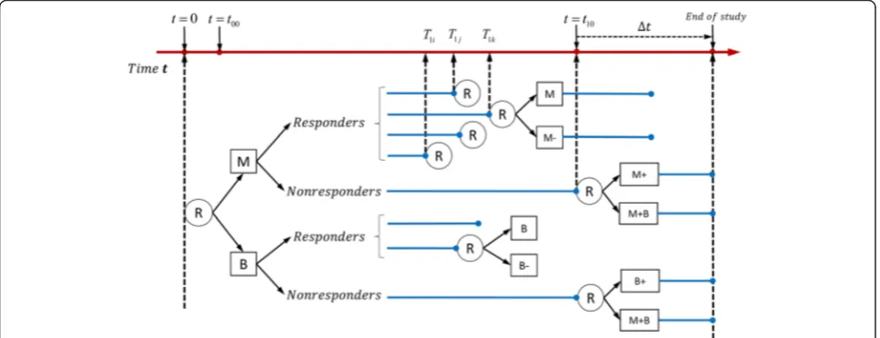
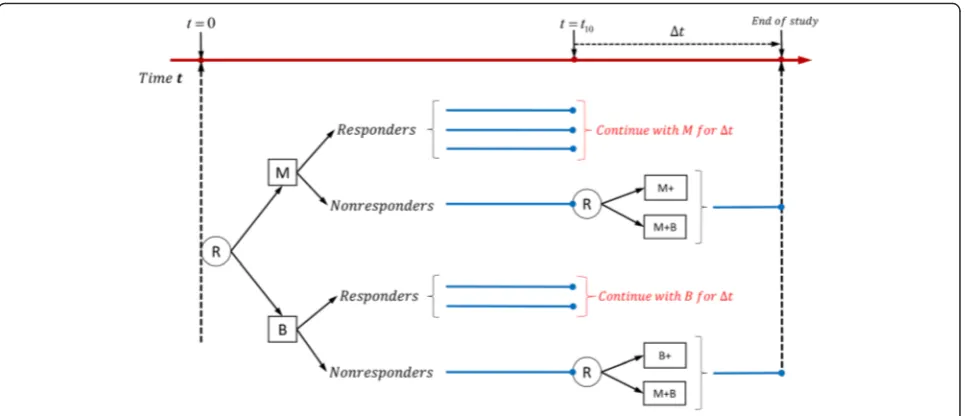
Figures 1 and 2 illustrate the proposed time-varying designs. Both two-stage time-varying SMARTs were de-signed to provide data regarding how the intensity and combination of two types of interventions might be adapted to a subject’s progress in a cost- and time-efficient manner.

In the first example (see Fig. 1), suppose medication (M) and behavioral intervention (B) are two initial inter-vention options for individuals who are heavy smokers (e.g., those who smoke more than or equal to 25 ciga-rettes per day). The number of cigaciga-rettes a subject smokes per day is the outcome of interest and is mea-sured at the beginning of the study, at several intermedi-ate time points and at the end of the study. Let Y0

denote the number of cigarettes a subject smoked per day at the beginning of the study (t = 0). Subjects are randomly assigned to the medication or the behavioral interventions at the beginning of the study. Monitoring the outcome of interest begins at a pre-fixed time point (e.g. one week after the initial randomization and is denoted as t00) after the initial intervention is imple-mented, and t10 denotes the time point at which those

who did not respond to a first-stage intervention are

randomized. A subject is considered a responder to the first-stage intervention if there is a significant decrease in the number of cigarettes he/she smoked per day (e.g., the decrease in the number of cigarettes smoked per day is above a pre-fixed threshold, C) at an intermediate time point T1, beforet10. Thus,T1is a random variable

of time and varies among responders. A subject is classi-fied as a non-responder if the decrease in the number of cigarettes he or she smoked per day by t10 is below C.

Therefore, all the non-responders are given the first-stage intervention for a fixed time period oft10(e.g., the

first month of initial interventions), which can be seen as the right-censored time point. LetY1denote the

num-ber of cigarettes smoked per day at the end of the first-stage intervention.

An indicator variable δ is defined as δ=I(T1<t10),

whereI(⋅) is the indicator function that takes the value 1 if T1<t10 (i.e., if the subject is a responder) and the

value 0 if T1≥t10 (i.e., if the subject is a

non-responder). A responder is re-randomized either to continue with the first-stage intervention (M or B) or to receive the first-stage intervention at a reduced intensity (M- or B-); whereas a non-responder is re-randomized to receive the first-stage option at an increased intensity (M+ or B+) or augmented with the other type of intervention (i.e., adding a behavioral intervention for those who started with medication or adding medication for those who started with a behav-ioral intervention). We let all the subjects in this design stay on their second-stage interventions for a fixed time period, Δt (e.g., one month). Therefore, for a subject whose first-stage intervention time isT1, the total study

time is T1 +Δt, which we denote asT2. For each

par-ticipant,Y2 is the final measurement of the number of

cigarettes smoked per day atT2; see Fig. 1).

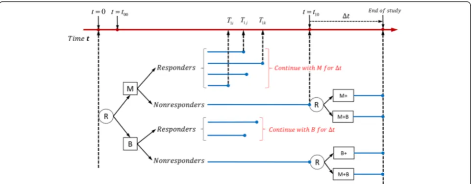
The design illustrated in Fig. 2 is similar to that in Fig. 1 except that all the responders continue with their first-stage intervention options (i.e., each responder receives the same intervention after the response time pointT1) in the second stage (see Fig. 2).

The adaptive interventions that are embedded within the two SMART designs in Figs. 1 and 2 are listed in Additional file 1: Tables S1 and S2.

Analytic approach

LetA1andA2be the indicators of the first- and second-stage intervention options, respectively. For each indi-vidual, we observe the data (Y0,A1,T1,Y1,A2,Y2,T2,δ). The outcomes of interest are the longitudinal measure-mentsY0,Y1, andY2, which are fitted with a linear mixed model, assuming they share the same random intercepts at the subject level. Because the intervention options and their durations change over time in this design, we first proposed a straightforward time-varying mixed ef-fects model (TVMEM) to analyze the outcomes. In this approach, the duration of time a treatment is adminis-tered is used as a covariate in the model. Such an ap-proach is better than the apap-proaches that ignore the time component of the intervention (i.e., the duration of the intervention influences its effect). However, the time duration is a random variable and one may gain statis-tical efficiency by treating it as a dependent variable in the modeling. Therefore, we also proposed a joint-modeling approach that simultaneously postulates a linear mixed effects model for the longitudinal measure-ments Y= (Y0,Y1,Y2) and a Cox model for the survival timeT1. In particular, we fit a survival submodel for T1

Analytic models

Time-varying mixed effects model of Y = (Y0, Y1, Y2)

A linear TVMEM is fitted to the longitudinal outcomes, with interventions and their interactions and durations included as predictors. For each individualiin the study, we have

YiðtÞ ¼miðtÞ þεiðtÞ ¼ZiηðtÞ þXiðtÞβðtÞ þbiþεiðtÞ

¼ZiηðtÞ þβ0ðtÞ þβ1ðtÞA1iðtÞ þβ2ðtÞA2iðtÞ

þβ3ðtÞtþβ4ðtÞA1iðtÞ⋅A2iðtÞ þbiþεiðtÞ

ð1Þ

wheremi(t) is the unobserved true value of the longitudinal

outcome at time point t, andbiis the subject-level random

effects and is assumed to be normally distributed with a mean of zero and variance ofσb2;Ziis a vector of the

base-line covariates (e.g., age, sex, comorbidities, etc.) with a cor-responding vector of the regression coefficientsη(t);Xi(t) is

the vector of the first-stage and second-stage intervention options, their interactions, and duration of intervention with a corresponding vector of the regression coefficients β(t). Finally,εi(t) is the error term at time t and is assumed

to be normally distributed and independent ofbi.

In our study design, we consider three time points at which the outcomes of interest are measured: t = 0,T1i

andT2i, whereT1iand T2iare the respective time points

at which individual i completes the first- and second-stage interventions. Therefore, A1i(t) takes the value of

A1i at timesT1i and T2i and is equal to 0 at t= 0, and

A2i(t) takes the value of A2i at T2i and is equal to 0 at

time points 0, and T1i. In this way, η(t) and β(t) are

piecewise linear fixed coefficients; therefore, model (1) at the three time points is equivalent to the following three linear mixed-effects submodels:

Y0i ¼Yið Þ ¼0 mið Þ þ0 εið Þ0

¼Ziηð Þ þ0 XTið Þ0 βð Þ þ0 biþεið Þ0

¼Ziη0þβ00þbiþε0i ð2Þ

Y1i¼YðT1iÞi¼miðT1iÞ þεiðT1iÞ

¼ZiηðT1iÞ þXTiðT1iÞβðT1iÞ þbiþεiðT1iÞ ¼Ziη1þβ01þβ11A1iþβ31T1iþbiþε1i

ð3Þ

and

Y2i ¼YiðT2iÞ ¼miT2iþεiðT2iÞ

¼ZiηðT2iÞ þXTiðT2iÞβðT2iÞ þbiþεiðT2iÞ ¼Ziη2þβ02þβ12A1iþβ2A2iþβ32T2i

þβ4A1i⋅A2iþbiþε2i

¼Ziη2þβ02þβ12A1iþβ22A2Riþβ23A2NRi þβ32T2iþβ41A1i⋅A2Riþβ42A1i⋅A2NRi

þbiþε2i ð4Þ

where in equations (2) through (4),Y0i,Y1i and Y2i are

the outcome values at time 0,T1i and T2i, respectively;

A1iis the indicator of the first-stage intervention

op-tions (−1 for M and +1 for B), A2i= (A2Ri,A2NRi) is

the indicator vector for the second-stage interven-tion opinterven-tions, where A2Ri is the indicator for the

second-stage intervention options for the responders to the first-stage intervention (1 = continue the initial intervention; −1 = reduce the intensity of the initial intervention) and A2NRi is the indicator for the

second-stage intervention options for the non-responders (1 = increase the initial intervention; −1 = augment the initial intervention with the other type of intervention), with A2Ri =0 for non-responders

and A2NRi =0 for responders. A1i⋅A2Ri and A1i⋅

A2NRi are the interaction effects of the first-stage

intervention and second-stage intervention among responders and non-responders, respectively, in the submodel of Y2i (i.e., submodel (4)).

Parameters η0,η1,η2 and β00,β01,β02 are the coeffi-cients of the baseline covariates and intercepts at time points 0,T1i and T2i, respectively; submodel (2)

includes only baseline covariates as predictors for the outcomes at the beginning of the study (i.e., Y0i

at t = 0); submodel (3) models the outcome of inter-est at the intermediate time point of the study (i.e.,

Y1i at t= T1i) and includes covariates A1i and T1i, for

which the corresponding coefficients β11 and β31 ac-count for the direct effect of A1i and indirect effects

through T1i on Y1i; submodel (4) includes all the

main and interacting effects of the intervention op-tions at each stage and the duration T2i (T2i=T1i

+Δt) as predictors, for which the coefficients β12 and β32 account for the delayed effect of A1i and

de-layed indirect effects of A1i through T2i. The

coeffi-cients β2= (β22,β23) and β4= (β41,β42) account for the effects of the second-stage interventions and the effects of their interactions with the first-stage inter-ventions on the final outcome Y2i (measured at the

end of the study,T2i).

The conditional expectations for models (1)-(4) are provided in Additional file 2. We also provided condi-tional expectations of the final outcomes for each of the eight embedded adaptive interventions in the SMART design of Fig. 1 and four embedded adaptive interventions in the SMART design of Fig. 2 [see Additional file 2].

Joint model

In addition to the TVMEM, we postulate a relative risk model forT1i(time to the event of interest) as

hið Þ ¼t h0ð Þt exp γ1A1iþγ2Wiþαmið Þ0

ð5Þ

where Wi is a vector of the baseline covariates, which

is the baseline risk function. The underlying longitudinal measurementmi(0) at baseline (i.e., at time point t = 0), as

approximated by the TVMEM, and at the first-stage inter-vention A1i are included as predictors in model (5)

be-cause the time point at which an individual responds to the first-stage intervention (i.e.,T1i) depends only on the

type of first-stage intervention the subject received and the baseline characteristics.

We jointly estimate the coefficients in models (1) and (5) by using the maximum likelihood estimation method. To define the joint distribution of the time-to-event and longitudinal outcomes, we assume that the random effect bi underlies both the longitudinal and survival

processes for each subject. This means that the random effect accounts for both the association between the longitudinal and event outcomes and the correlation between the repeated measurements in the longitudinal process. We also assume that the longitudinal outcomes {Y0i,Y1i,Y2i} are independent of the timeT1i conditional

on the random effect bi. Therefore, the joint likelihood

contribution for the ith subject can be formulated as

p(T1i,δi,Yi;θ) =

Z

p Tð 1i;δijbi;β;γ;α;ηÞ

Y

j

p Yi tij jbi;β;η

" #

p bð i;;σbÞdb,

where p{Yi(tij)|bi;β,η} is the univariate normal density

for the longitudinal responses at time point tij, which is

the element from the vector ti= {tsi}2s= 0= {0,T1i,T2i};

p(bi;σb) is the normal density with standard deviationσb

for the random effectsbi; andp(T1i,δi|bi;β,γ,α,η) is the

likelihood for the time to the intermediate outcome and can be written as p(T1i,δi|bi;β,γ,α,η) =

hiðT1ijmið Þ0 ;β;γ;α;ηÞ

f gδi⋅ _S

i(T1i|mi(0),A1i;β,γ,α,η) =

hiðT1ijmið Þ0 ;β;γ;α;ηÞ

f gδi⋅ _{exp −}

Z T1i

0

hiðsjmið Þ0;β;γ;α;ηÞds

,

where δi=I(T1i<t10). Parameters in the model are

esti-mated by maximizing the corresponding log-likelihood function with respect to (β,γ,α,η). We obtained the maximum likelihood estimates using the R package “JM” [30].

The parameters (β12,β22,β23,β32,β41,β42) in submodel (4) (i.e., the model of final outcome _Y2) are of primary

interest and were estimated using the two approaches described above.

The data organization and implementation of these methods is presented in Additional file 3.

Simulations

For the example illustrated in Fig. 1, we considered two simulation scenarios in which Y0 and Y1 were simulated using submodels (2) and (3), respectively, and Y2 was simulated with and without the

inter-action terms (A1i⋅A2Ri and A1i⋅A2NRi) in submodel

(4). In both scenarios, we simulated 500 replicates of

n= 1000 individuals, and randomly assigned subjects (with probability .5) to one of the two first-stage in-terventions (i.e., A1 to be equal to 1 [behavioral

intervention] or −1 [medication]). Responders and non-responders to the initial interventions were then re-randomized (with probability .5) to one of the corresponding second-stage intervention options (i.e.,

A2R and A2NR were randomly assigned to be 1 or −1

and A2R =0 for non-responders and A2NR =0 for

re-sponders; see Fig. 1). In both scenarios, the random effects {bi}in= 1 for subjects i= 1, 2,…,n were

gener-ated from the normal distribution with a mean of 0 and a standard deviation of 5, and baseline outcomes {Y0i}in= 1 were simulated using submodel (2) with

pa-rameters β00= 10 and ε0i~N(0, 42). The intermediate

outcomes {Y1i}in= 1 were simulated using submodel (3)

with parameters β01= 1, β11= 0.2, and β31= 0.1 in the first scenario; whereas outcomes {Y1i}in= 1 in the

second scenario were simulated with β01= 1,β11= 0.6, and β31= 0.1, with a standard deviation of 5 (i.e.,

ε1i~N(0, 52) in both scenarios and satisfying the

conditions Y0i−Y1i≥9 (C = 9) if subject i is a

re-sponder and Y0i−Y1i< 9 if subject i(i= 1, 2,…n) is a

non-responder.

The time points T1i were generated from a

left-truncated Weibull distribution (left-truncated fromt00=0.1, the start time for monitoring), with shape = 1 and scale= exp{γ0+γ1A1i+αmi(0)}, where γ0=−1.5, γ1=

0.4, and α= 0.25, and those for whom T1i was greater

than 1 (non-responders), were assigned T1i=t10= 1

(the maximum time the first-stage intervention is administered [t10]). The indicator of response status was then defined by δi=I(T1i< 1). The final outcomes

Y2i(i= 1,…,n) were generated using submodel (4), with

ε2i~N(0, 52). The values of the other parameters in

submodel (4) are reported in Table 1 (without interac-tions) and Table 3 (with interacinterac-tions).

For the intervention strategy depicted in Fig. 1, there are eight adaptive interventions imbedded in the design and represented by the three indicators

A1,A2R, and A2NR. For example, in adaptive

interven-tion (A1,A2R,A2NR) = (−1, 1, 1), participants are

ini-tially randomized to the medication (A1=−1); those

who respond are re-randomized to continue on the medication (A2R= 1) and those who do not respond

are re-randomized to increased medication (A2NR= 1).

Another example of an adaptive intervention is (A1,

A2R,A2NR) = (1, 1, −1), in which participants are

ini-tially randomized to a behavioral intervention (A1= 1);

those who respond are re-randomized to continue on the behavioral intervention (A2R= 1), and those who

For the design in Fig. 2, only the non-responders are re-randomized in the second stage. Therefore, there are four embedded adaptive interventions in this design, which are represented by the vector of two indicators (A1,A2NR). For example (−1,−1) represents the adaptive

intervention in which participants are initially random-ized to medication (A1=−1) and those who do not re-spond are re-randomized to the augmented arm (M + B,

A2NR=−1), whereas responders continue on the

medi-cation arm.

Using this design, we also simulated the treatment of 1000 subjects. However, instead of using equal ability allocations as in Fig. 1, we used unequal prob-ability allocations at both stages. Specifically, each of the 1000 subjects were initially assigned to either A1= −1 (medication) or A1 =1 (behavioral intervention) with probabilities 0.4 and 0.6, respectively. Then, the non-responders were re-allocated into eitherA2NR=−1

(augmented first-stage intervention, M + B) or A2NR =1

(intensified first-stage intervention, M+ or B+) with probabilities 0.55 and 0.45, respectively; whereas all re-sponders were continued on their initial interventions (therefore, A2R =0) in their second stage. Random

effects (bi), errors (εi), and longitudinal outcomes (Y0i,

Y1i(i= 1,…,n)) were generated as described for Fig. 1.

The final outcomes,Y2i(i= 1,…,n), were also generated

using submodel (4), but without the variableA2Ri, with

the parameter values reported in Tables 5 and 7 for the two scenarios, respectively. In the first scenario, out-comes Y2i(i= 1,…,n) were simulated without

inter-action terms and with the parameter values shown in Table 5; in the second scenario, outcomes Y2i(i= 1,…,

n) were simulated with interaction terms and with the parameter values shown in Table 7.

An alternate simulation approach

For the design illustrated in Fig. 1, we performed an alternate simulation approach that does not simulate

Table 1Simulation results for the design in Fig. 1: the estimated means, based on 500 replicates, are reported for coefficients in model (4)

Parameter estimation

β12 β22 β23 β32

(first-stage interventionsA1)

(second-stage interventions for respondersA2R)

(second-stage interventions for non-respondersA2NR)

(time of interventionT2)

True value 0.4 0.5 0.5 2

Joint Model Estimate 0.407 0.503 0.502 1.790

MSE 0.011 0.029 0.016 0.147

CI% 97.8 % 95.0 % 96.8 % 94.2 %

Length of CI

0.478 0.674 0.538 1.447

TVMEM Estimate 0.275 0.503 0.501 4.073

MSE 0.026 0.030 0.017 4.400

CI% 88.0 % 95.6 % 97.0 % 0.0 %

Length of CI

0.484 0.695 0.549 1.436

CI%: Coverage probability of the 95 % confidence interval MSEmean squared error

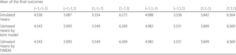
Table 2Simulation results for the design in Fig. 1: the estimated means, based on 500 replicates, are reported for the final outcomes of the eight adaptive interventions embedded in the design

Mean of the final outcomes

(₋1,-1,-1) (₋1,-1,1) (1,-1,-1) (1,-1,1) (₋1,1,-1) (₋1,1,1) (1,1,-1) (1,1,1)

Simulated means

4.538 5.087 5.554 6.275 4.988 5.536 5.842 6.564

Estimated means by Joint model

4.543 5.093 5.549 6.269 4.982 5.531 5.849 6.569

Estimated means by TVMEM

values for_T1ifrom the Weibull distribution. Instead, we

considered a situation in which values of Y1i are

moni-tored and T1i is the value for which the Y1i crosses the

pre-specified boundary condition for the first time. In this simulation approach, random effects {bi}in= 1 and

error termsε0,ε1and ε2were all simulated the same way as described above. Baseline outcomes {_Y0i}in= 1are

simu-lated using submodel (2) withβ00= 2 andε0i~N(0, 22).

Furthermore, we defined an individuali, as a responder if he/she had a certain percentage reduction in the inter-mediate outcome value, Y1i, compared to his/her

base-line valueY0i. This may be a more appropriate definition

of responders in some practical scenarios than a simple reduction by a fixed amount (e.g., C = 9) as was used in the previous simulations. In this simulation, those with a 40 % reduction from their baseline values were considered responders. The parameter values used for submodel (3) wereβ01=−2,β11=−0.5, andβ31= 5 . For an individuali,

we first simulated ε1i ~N (0, 22), and calculated T1*i for

which the β01+β11A1i+β31T*1i+bi+ε1i equals the 40 %

reduction from Y0i, the baseline value. Therefore, we

define_T1i=t00, if T*1i<t00; T1i=T1*i, if t00≤T1*i≤t10; and T1i=t00, if T*1i≥t10. Then,T1i is substituted in the right

side of equation (3) to obtain the value ofY1ifor the

indi-vidual _i(_i= 1,…,_n). The final outcomes _Y2i(i= 1,…,n)

were generated using submodel (4), withε2i ~ N (0, 22).

As previously, we simulated 500 replicates of n = 1000 in-dividuals in each trial, and randomly assigned subjects (with probability 0.5) to one of the two first-stage inter-ventions (i.e.,A1to be equal to 1 [behavioral intervention]

or −1 [medication]). Responders and non-responders to the initial interventions were then re-randomized (with probability 0.5) to one of the corresponding second-stage intervention options (i.e., _A2R and A2NR were randomly

assigned to be 1 or−1 andA2R=0 for non-responders and

A2NR=0 for responders; see Fig. 1).

Table 3Simulation results for the design in Fig. 1: the estimated means, based on 500 replicates, are reported for coefficients in model (4) with interactions

Parameter estimation

β12 β22 β23 β32 β41 β42

(first-stage interventionsA1)

(second-stage interventions for respondersA2R)

(second-stage interventions for non-respondersA2NR)

(time of interventionT2)

(interaction termA1.A2R)

(interaction termA1.A2NR)

True value −0.4 0.5 0.4 2.0 0.55 −0.40

Joint model Estimate −0.381 0.490 0.389 1.626 0.542 −0.397

MSE 0.014 0.038 0.019 0.305 0.037 0.019

CI% 97.4 % 95.6 % 96.8 % 87.0 % 96.8 % 98.0 %

Length of CI

0.521 0.789 0.593 1.671 0.789 0.593

TVMEM Estimate −0.530 0.489 0.390 4.122 0.542 −0.396

MSE 0.029 0.039 0.020 4.697 0.037 0.020

CI% 88.2 % 95.8 % 96.4 % 0.0 % 97.0 % 97.8 %

Length of CI

0.525 0.809 0.605 1.618 0.809 0.605

CI%: Coverage probability of the 95 % confidence interval MSEmean squared error

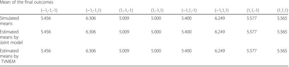
Table 4Simulation results for the design in Fig. 1: the estimated means, based on 500 replicates, are reported for the final outcomes of the eight adaptive interventions embedded in the design with interactions in model (4)

Mean of the final outcomes

(₋1,-1,-1) (₋1,-1,1) (1,-1,-1) (1,-1,1) (₋1,1,-1) (₋1,1,1) (1,1,-1) (1,1,1)

Simulated means

5.456 6.306 5.009 5.000 5.400 6.249 5.577 5.565

Estimated means by Joint model

5.456 6.306 5.009 5.000 5.400 6.249 5.577 5.565

Estimated means by TVMEM

We evaluated the performance of our two proposed analytic approaches in these simulated data sets by measuring the (a) means of the estimates of each of the adaptive interventions embedded in the design, (b) par-ameter estimates in the model, (c) mean squared error (MSE), (d) estimated coverage probability of the 95 % confidence interval, and (e) length of the confidence interval.

Using these simulations parameters, we simulated two trials with identical sample sizes: (a) the time-varying SMART design and (b) the standard SMART design. We evaluated the performance of the time-varying SMART design and an analogous standard SMART design by measuring the (a) power to select the optimal embedded intervention, and (b) associated cost.

Results

Tables 1-4 show the results of the two simulation sce-narios based on the design shown in Fig. 1. Similarly, Tables 5-8 show the results of the two simulation scenarios for the design in Fig. 2.

In Table 1 the true parameters were the coefficient of the first-stage interventions, β12= 0.4; coefficient of the second-stage intervention for responders, β22= 0.5; coefficient of the second-stage intervention for non-responders,β23= 0.5; and coefficient of T2, the total time

of the first- and second-stage interventions, β32= 2. The estimates obtained using TVMEM were^β₁₂¼0:275; β^₂₂ ¼0:503; ^β₂₃¼0:501; and β^₃₂¼4:073 , while the estimates obtained using the joint model were ~β₁₂ ¼0:407; β22~ ¼0:503; β23~ ¼0:502; and β32~ ¼1:790 . Both approaches estimated coefficients β22 and β23 accurately. The parametersβ12andβ32 were estimated accurately using the joint model, but poorly using the TVMEM. Similarly, in terms of the MSE, the length of the 95 % confidence interval, and the estimated coverage probability of the 95 % confidence interval, both approaches performed similarly for estimatingβ22 and β23, but joint modeling performed better for esti-matingβ12andβ32. For example, forβ12, the estimated coverage probability obtained using the TVMEM was 88 %; whereas that obtained from the joint model was 97.8 %.

For each of the eight embedded adaptive interventions in the design, Table 2 shows that both approaches accur-ately estimated the means of the final outcome,

E[Y2|(A1,A2R,A2NR)]. For example, the simulated means

of the adaptive interventions (A1,A2R,A2NR) = (−1,−1,−

1), (−1, 1, 1), and (1, 1, 1) were 4.538, 5.536, and 6.564, respectively, and the estimated means were 4.543, 5.531, and 6.569, respectively, using the TVMEM and joint model.

Tables 3 and 4 show results similar to those in Tables 1 and 2, respectively. In Table 3, the coefficient of inter-action of the first-stage interventions and second-stage interventions among responders is denoted by

β41, and the coefficient of interaction of the first-stage interventions and second-stage interventions among non-responders is denoted by β42. As shown in Table 3, both TVMEM and joint modeling accurately estimated parameters β22, β23, β41, and β42, with little difference in the MSE, estimated coverage probability, and length of the 95 % confidence interval. However, as in Table 1, the joint modeling approach estimated

β12 and β32 more accurately than the TVMEM ap-proach. For example, the true coefficient of T2 was β32= 2.0, which was poorly estimated as 4.122 using the TVMEM and estimated as 1.626 using the joint model. Table 4 shows that the estimated means of the eight adaptive interventions obtained from both analytical approaches were identical and close to the simulated means up to the third decimal.

Similar trends were observed in Tables 5-8 for the two simulations of Fig. 2. β12 and β32 were better estimated using the joint modeling approach, whereas all the other parameters and the means of the final outcomes of the four adaptive interventions embedded in the design were accurately estimated using both approaches.

In Table 5, the true coefficient values of β12 =0.450 and β32 =2.0 were estimated as ^β₁₂¼0:388 and β^₃₂ ¼4:046 using the TVMEM, and as β~₁₂ ¼0:456 and ~

β32¼1:767 using the joint model. Coefficient β23 was

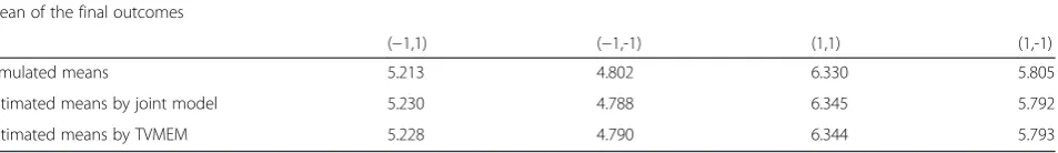
accurately estimated using both models. As for the four adaptive interventions (i.e. (A1,A2NR) = (−1,1),

(−1,-1), (1, 1) and (1, −1)) embedded in the design of Fig. 2, Table 6 shows that the simulated means were 5.213, 4.802, 6.330, and 5.805, respectively, and the estimated means were 5.228, 4.790, 6.344, and 5.793, respectively, using the TVMEM, and 5.230, 4.788, 6.345, and 5.792, respectively, using the joint model.

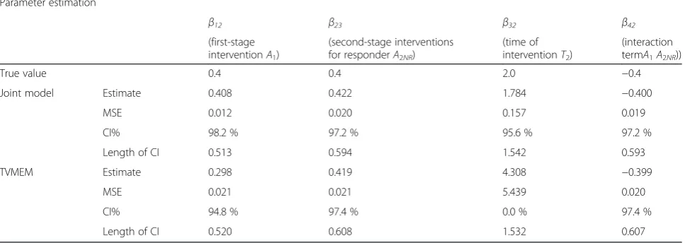
In Table 7 shows that the true parameters β12 =0.40 and β32 =2.0 were respectively estimated as β^₁₂ =0.298 and^β32 =4.308 using the TVMEM, and asβ~₁₂ =0.408 and ~

β32 =1.784 using the joint model. The other two

parameters, β23 and β42, were accurately estimated using both approaches. Table 8 shows that the means were accurately estimated using both approaches.

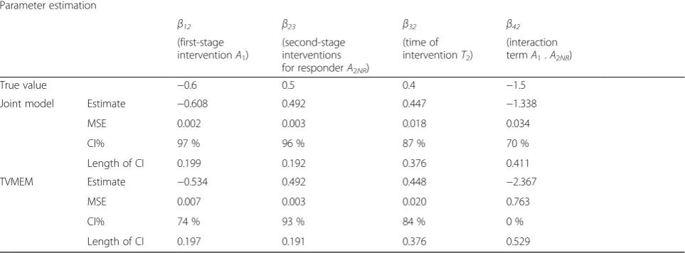
TVMEM, and as β~₁₂ =−0.608 and ~β₃₂ = −1.338 using the joint model. Coefficients β22, β23 and the means of the final outcomes of the eight adaptive interven-tions embedded in the design were accurately esti-mated using both approaches (Table 10).

Comparison of power between the time-varying SMART design and the standard SMART design

We analyzed the time-varying SMART design’s ability to select the most optimal embedded intervention and compared the associated power to that of the standard SMART design. We performed the compari-son by conducing two trials with identical sample sizes and intervention effects using (a) the time-varying SMART design and (b) the standard SMART design. Figure 3 represents the standard SMART design that is analogous to the time-varying SMART design depicted in Fig. 1. The major difference be-tween the two designs is that in the time-varying SMART design, a responder is re-randomized to the second-stage intervention at a random response time

T1 (< t10); whereas in the standard SMART design,

everyone is re-randomized at a fixed time point t10.

Responders are defined similarly in both designs. In our example, a subject is considered a responder to the first-stage intervention if there is a significant decrease in the number of cigarettes the person smoked per day. The second-stage intervention is identical for both designs.

For both designs, we calculated the percentage of times that the best embedded intervention is selected (i.e., the power of the design). We simulated six parameter scenarios: the true parameters for the coefficient of the first-stage interventions, β21; coefficient of the second-stage intervention for re-sponders, β22; coefficient of the second-stage inter-vention for non-responders, β23; coefficient of _T2,

the total time of the first- and second-stage inter-ventions, β32; coefficient of interaction of the first-stage interventions and second-first-stage interventions among responders β41; and the coefficient of inter-action of the first-stage interventions and second-stage interventions among non-responders β42. The

Table 5Simulation results for the design in Fig. 2: the estimated means, based on 500 replicates, are reported for coefficients in model (4)

Parameter estimation

β12 β23 β32

(first-stage interventionsA1)

(second-stage interventions for non-respondersA2NR)

(time of interventionT2)

True value 0.450 0.40 2.0

Joint model Estimate 0.456 0.441 1.767

MSE 0.013 0.017 0.168

CI% 95.6 % 95.6 % 93.6 %

Length of CI 0.482 0.536 1.452

TVMEM Estimate 0.388 0.439 4.046

MSE 0.016 0.017 4.297

CI% 94.0 % 96.0 % 0.0 %

Length of CI 0.489 0.547 1.442

CI%: Coverage probability of the 95 % confidence interval MSEmean squared error

Table 6Simulation results for the design in Fig. 2: the estimated means, based on 500 replicates, are reported for the final outcomes of the four adaptive interventions embedded in the design

Mean of the final outcomes

(−1,1) (−1,-1) (1,1) (1,-1)

Simulated means 5.213 4.802 6.330 5.805

Estimated means by joint model 5.230 4.788 6.345 5.792

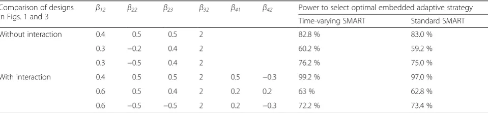
simulated values of each of these parameters are reported in Tables 11 and 12. The simulation results are based on 500 replicates and are shown in Table 11 for comparing the two designs in Fig. 1 (time-varying SMART) and Fig. 3 (analogous standard SMART). Overall, both designs were equally effective in selecting the optimal embedded adaptive interven-tion. For example, when β21= 0.4, β22= 0.5, β23= 0.5 and β32= 2, using the joint model and implementing the time-varying SMART design showed 82.8 % power to select the optimal embedded adaptive inter-vention; whereas the power associated with the stand-ard SMART design was 83.0 %. Similar results were obtained when comparing the time-varying SMART design in Fig. 2 and the standard SMART design in Fig. 4 (see Table 12).

Comparison of the cost associated with conducting the time-varying SMART design versus that associated with conducting the standard SMART design

To assess the cost associated with the conducting trials using these two competing designs, we consid-ered a linear cost function for both SMART designs.

Let c1 and c2 be the cost of the medication (M) and behavioral intervention (B), respectively. Additionally, we assumed that the reduced and increased intensity of the first-stage intervention are at half and twice the cost of the first-stage intervention, respectively, and that augmentation of the first-stage intervention in the second stage (M + B) has the cost c1+ c2. Using these parameters, the cost for the time-varying SMART design in Fig. 1 is

cost¼c1 X

A1i¼M

T1i 0 @

1 Aþc1

X

A2i¼M

Δt 0 @

1 Aþ c1

2 X

A2i¼M−

Δt 0 @

1 A

þð2c1Þ X

A2i¼Mþ

Δt 0 @

1 Aþ

c2 X

A1i¼B

T1i 0 @

1 Aþc2

X

A2i¼B

Δt 0 @

1 Aþ c2

2 X

A2i¼B−

Δt 0 @

1 A

þð2c2Þ X

A2i¼Bþ

Δt 0 @

1

Aþðc1þc2Þ X

A2i¼MþB

Δt 0 @

1 A_;

Table 7Simulation results for the design in Fig. 2: the estimated means, based on 500 replicates, are reported for coefficients in model (4) with interactions

Parameter estimation

β12 β23 β32 β42

(first-stage interventionA1)

(second-stage interventions for responderA2NR)

(time of interventionT2)

(interaction termA1A2NR))

True value 0.4 0.4 2.0 −0.4

Joint model Estimate 0.408 0.422 1.784 −0.400

MSE 0.012 0.020 0.157 0.019

CI% 98.2 % 97.2 % 95.6 % 97.2 %

Length of CI 0.513 0.594 1.542 0.593

TVMEM Estimate 0.298 0.419 4.308 −0.399

MSE 0.021 0.021 5.439 0.020

CI% 94.8 % 97.4 % 0.0 % 97.4 %

Length of CI 0.520 0.608 1.532 0.607

CI%: Coverage probability of the 95 % confidence interval; MSE: mean squared error

Table 8Simulation results for the design in Fig. 2: the estimated means, based on 500 replicates, are reported for the final outcomes of the four adaptive interventions embedded in the design with interactions in model (4)

Mean of the final outcomes

(−1,1) (−1,-1) (1,1) (1,-1)

Simulated means 5.487 4.622 6.032 6.059

Estimated means by joint model 5.502 4.610 6.047 6.046

and the cost for the corresponding standard SMART in Fig. 3 is

cost¼c1 X

A1i¼M

t10 0 @

1 Aþc1

X

A2i¼M

Δt 0 @

1 Aþ c1

2

X

A2i¼M−

Δt 0 @

1 Aþ

2c1

ð Þ X

A2i¼Mþ

Δt 0 @ 1 Aþ c2 X

A1i¼B

t10 0 @

1 Aþc2

X

A2i¼B

Δt 0 @

1 Aþ c2

2 X

A2i¼B−

Δt 0 @

1 Aþ

2c2

ð Þ X

A2i¼Bþ

Δt 0 @

1

Aþðc1þc2Þ X

A2i¼MþB

Δt 0 @

1 A_:

Similarly, the cost for the time-varying SMART in Fig. 2 is

cost¼c1

X

A1i¼M

T1i

0 @

1 Aþc1

X

A2i¼M

Δt 0 @

1 Aþð2c1Þ

X

A2i¼Mþ

Δt 0 @ 1 Aþ c2 X

A1i¼B

T1i

0 @

1 Aþc2

X

A2i¼B

Δt 0 @

1 Aþð2c2Þ

X

A2i¼Bþ

Δt 0 @

1 Aþ

c1þc2

ð Þ X

A2i¼MþB

Δt 0 @

1 A_;

and the cost for the corresponding standard SMART in Fig. 4 is

Fig. 3Example of standard SMART design with equal probability allocation: each participant is randomized twice

Table 9Simulation results from the alternative simulation approach: the estimated means, based on 500 replicates, are reported for coefficients in model (4)

Parameter estimation

β12 β23 β32 β42

(first-stage interventionA1)

(second-stage interventions for responderA2NR)

(time of interventionT2)

(interaction termA1.A2NR)

True value −0.6 0.5 0.4 −1.5

Joint model Estimate −0.608 0.492 0.447 −1.338

MSE 0.002 0.003 0.018 0.034

CI% 97 % 96 % 87 % 70 %

Length of CI 0.199 0.192 0.376 0.411

TVMEM Estimate −0.534 0.492 0.448 −2.367

MSE 0.007 0.003 0.020 0.763

CI% 74 % 93 % 84 % 0 %

Length of CI 0.197 0.191 0.376 0.529

cost¼c1 X

A1i¼M

t10 0 @

1 Aþc1

X

A2i¼M

Δt 0 @

1 Aþð2c1Þ

X

A2i¼Mþ

Δt 0 @

1 Aþ

c2 X

A1i¼B

t10 0 @

1 Aþc2

X

A2i¼B

Δt 0 @

1 Aþð2c2Þ

X

A2i¼Bþ

Δt 0 @

1 Aþ

c1þc2

ð Þ X

A2i¼MþB

Δt 0 @

1 A_:

Note that in the above equations, T1i= t10 for

non-responders, and ðc1þc2Þ X

A2i¼MþB

Δt 0

@

1

Ais the cost of the

second stage for all the subjects assigned to the inter-vention M + B.

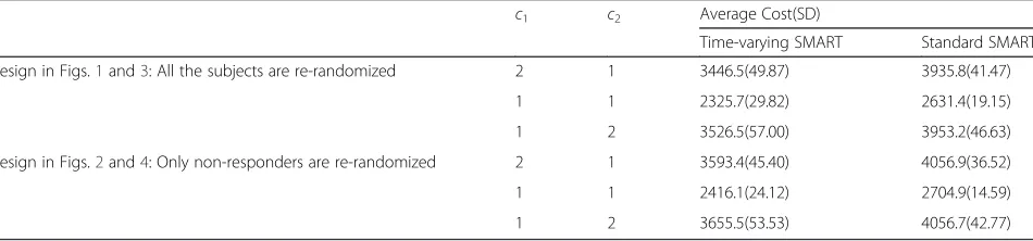
Figure 5 shows the cost as a function of c1 and c2, where red represents the cost of the time-varying SMART design and blue represents the cost of the standard SMART design. We can see that the cost of the time-varying SMART is less than the cost of the standard SMART in all scenarios. Table 13 shows the average costs and standard deviations calculated at select values of c1 and c2 based on 1000 replicates. For ex-ample, when the unit costs are c1= 2 and c2= 1 for medication and behavioral intervention, the average cost of the time-varying SMART in Fig. 1 is 3446.5, with standard deviation 49.87, while the average cost of the corresponding standard SMART is 3935.8, with standard deviation 41.47. Thus, the cost of the standard SMART

is about 12 % higher than that of the time-varying SMART in this scenario.

Discussion

In the standard SMART design, the timing of allocating the intervention is generally ignored, which leads to a model of regression without the predictor of a time vari-able. Therefore, in this article, we proposed a time-varying SMART design that allows the re-randomization to the second-stage interventions to occur at different time points for different individuals. The two modeling approaches we proposed for analyzing data using such time-varying SMART designs provided good estimations of the means of the final outcomes of all the embedded interventions. However, the joint modeling approach provided more accurate parameter estimates and higher estimated coverage probability than the TVMEM, and thus we recommend the joint model for analyzing data generated from time-varying SMART designs.

In the examples illustrated in Figs. 1 and 2, a partici-pant was defined as a responder if there was a significant decrease in the number of cigarettes the participant smoked per day. One may question the validity of re-randomizing individuals who have a quick response to the first-stage intervention because such a response indi-cates the effectiveness of the intervention. However, if significant adverse effects are associated with the inter-vention (e.g., radiation therapy for many types of cancer is commonly associated with skin damage [31], fatigue [32, 33], diarrhea [34, 35], and rectal bleeding [36]), it is

Table 11Power to select the optimal embedded adaptive intervention strategy for designs in Figs. 1 and 3

Comparison of designs in Figs.1and3

β12 β22 β23 β32 β41 β42 Power to select optimal embedded adaptive strategy Time-varying SMART Standard SMART

Without interaction 0.4 0.5 0.5 2 82.8 % 83.0 %

0.3 −0.2 0.4 2 60.2 % 59.2 %

0.3 −0.5 0.4 2 76.2 % 75.0 %

With interaction 0.4 0.5 0.5 2 0.5 −0.3 99.2 % 97.0 %

0.6 0.5 0.4 2 0.2 0.2 63 % 62.8 %

0.6 −0.5 −0.5 2 0.2 −0.3 72.2 % 73.4 %

Table 10Simulation results from the alternative simulation approach: the estimated means, based on 500 replicates, are reported for the final outcomes of the eight adaptive interventions embedded in the design

Mean of the final outcomes

(−1,-1,-1) (−1,-1,1) (1,-1,-1) (1,-1,1) (−1,1,-1) (−1,1,1) (1,1,-1) (1,1,1)

Simulated means −0.208 −0.070 −1.589 −1.356 0.678 0.810 −0.918 −0.689

Estimated means by Joint model −0.203 −0.066 −1.595 −1.359 0.675 0.804 −0.915 −0.683

reasonable to shorten the duration of the intervention to avoid side effects. Therefore, the allocation strategy for the responders in the examples of the time-varying SMART design makes it more efficient than the stand-ard SMART design.

We proposed two approaches for analyzing the longi-tudinal outcomes obtained from the time-varying SMART design: the TVMEM and the joint model. According to the simulation results, the joint modeling approach better estimated the effects of the duration of the intervention (i.e.,T2) and the first-stage interventions

(i.e.,A1) in model (4). More specifically, the joint

model-ing approach had more accurate estimates, smaller MSEs, higher estimated coverage probabilities, and smaller 95 % confidence intervals (i.e., smaller estimated standard deviations) for the coefficients of the effects of the first-stage intervention and the time of intervention. Because we wanted to illustrate the cost efficiency of the proposed time-varying SMART design and its ability to select the optimal embedded adaptive intervention, we implemented a rather simplified linear mixed-effects submodels (2)-(4) of the more general TVMEM in

model (1). We showed that the joint model performs better than the TVMEM in analyzing the data collected from such time-varying SMART designs. The joint mod-eling approach extracts part of the information con-tained in the time of the response, which is a function of the first-stage treatment assignment. Also, the associ-ation between the longitudinal and event outcomes is accounted for by the random effect that underlies both the longitudinal and survival processes for each subject. Therefore, although complex, time-varying SMART de-signs may require more complicated models for time and an extra layer of joint modeling, and as such one would expect a better performance from joint modeling in general. Nevertheless, both modeling approaches per-formed well in estimating the other parameters and the mean of the final outcomes for each adaptive interven-tion embedded in the corresponding designs. Further-more, equation (1) is a general form of TVMEM, and in our study is equivalent to equations (2) ~ (4) at time points t= 0,T1i,T2i for each subject i. T1i is a

subject-specific random variable, and coefficients in equation (3) can also be subject-specific. However, in practice, Fig. 4Example of standard SMART design: only non-responders are re-randomized in the second stage

Table 12Power to select the optimal embedded adaptive intervention strategy for designs in Figs. 2 and 4

Comparison of designs in Figs.2and4.

β12 β23 β32 β42 Power to select optimal embedded adaptive strategy Time-Varying SMART Standard SMART

Without interaction 0.5 0.5 2 92.8 % 90.6 %

0.45 0.4 2 86.6 % 83.6 %

−0.2 0.2 2 68.4 % 66.2 %

With interaction 0.4 0.4 2 −0.4 98.2 % 97.4 %

0.2 0.2 2 −0.4 88.4 % 87.6 %

modeling coefficients to be subject-specific may lead to the estimation of too many parameters which, in some scenarios, may not be identifiable, particularly with small sample sizes. Therefore, as an initial attempt, we mod-eled T1i as a subject-specific random variable and the

coefficients as fixed parameters. For example, coeffi-cients β0(t), β1(t), β3(t) in equation (1) are fixed coeffi-cients β01,β11,β31 in equation (3), as model (1) is equivalent to submodel (3) at time point T1i. More

complicated models such as subject-specific and time-varying coefficients in submodels (2)-(4) can be consid-ered, if the sample sizes are large.

We also illustrated the effectiveness of the joint mod-eling approach in accurately estimating the parameters even when no specific model was assumed for the dur-ation of the first-stage intervention,T1i. The conclusions

were qualitatively similar as that in the simulation where Weibull model was assumed for the duration of the first-stage intervention.

In the scenarios we considered here, the time at which individuals were re-randomized was assessed only for responders to the first-stage intervention. However, one may also consider varying times for the non-responders and for the second-stage interventions. For example, a non-responder showing severe side effects or no trend towards achieving intermediate goals may be re-randomized sooner thant10. The analytic approaches for

such designs would be similar to the joint or

time-varying mixed effects models proposed in this manu-script, for example, with an extra submodel for the duration of the second-stage interventions.

Instead of randomization with certain pre-defined probabilities (e.g., in the first two simulation scenarios, randomization with probability 0.5 was used for both stages; in the last two scenarios, unequal randomization with probabilities 0.4(0.6) and 0.55(0.45) was used for the two stages, respectively), information concerning po-tential moderators could be used to tailor and assign the interventions. For example, the choice of the first-stage intervention options could depend on the severity of the subject’s smoking habit at the beginning of the study; whereas the choice of the second-stage interven-tion opinterven-tion could depend on the subject’s adherence to the first-stage intervention. The analysis of such a randomization scheme would require assigning weights for each subject [37].

We also compared the cost and power associated with selecting the optimal embedded adaptive intervention for the proposed time-varying SMART design versus that for the analogous standard SMART design. Our simulation results showed similar power for the two de-signs. We used a linear cost function to assess the cost efficiency of the proposed design and found that it can have substantially lower cost than the standard design. Several other forms of cost functions can be used to assess cost efficiency. However, as long as the cost is an Fig. 5The cost associated with implementing a standard SMART (blue) and equivalent time-varying SMART (red)

Table 13Examples of the average cost for time-varying SMART and the standard SMART

c1 c2 Average Cost(SD)

Time-varying SMART Standard SMART

Design in Figs.1and3: All the subjects are re-randomized 2 1 3446.5(49.87) 3935.8(41.47)

1 1 2325.7(29.82) 2631.4(19.15)

1 2 3526.5(57.00) 3953.2(46.63)

Design in Figs.2and4: Only non-responders are re-randomized 2 1 3593.4(45.40) 4056.9(36.52)

1 1 2416.1(24.12) 2704.9(14.59)

increasing function of time, the proposed time-varying SMART design will have lower cost than the standard SMART design. Therefore, the time-varying SMART de-sign can be used to study how the intensity and combin-ation of two types of interventions might be adapted to a subject’s progress in a cost- and time-efficient manner.

In our study, we assume that there is no unmeasured confounder. As suggested by Chakraborty and Murphy [38], the assumption of “no unmeasured confounders” holds in a SMART design if the randomization probabil-ities of A1 at most depend on the baseline covariates,

and the randomization probabilities of A2 at most

de-pend on the baseline covariates, the intermediate out-come, and A1. We performed additional simulations to

investigate the role of unmeasured confounders on the parameter estimations. From these simulations, we see that when the unmeasured confounders affect only T1

and Y1, the parameter estimation is still accurate

(Additional file 4: Table S4). However, when these un-measured confounders affectY2, there is bias in the

esti-mation ofT2(Additional file 4: Tables S5-S6).

In the ADHD SMART study discussed by Nahum-Shani et al. [20], a weighted average was applied to the final outcomes when their primary goal of the study was to compare the imbedded adaptive intervention options in the SMART. In our Time-Varying SMART study, we used regression-based methods to identify more efficient adaptive decision rules for each subject along with their longitudinal outcomes. Similar to the analytic process of the standard SMART design by Q-learning in which a regression model for the outcome is postulated at each decision as a function of the patient’s information to that point, our TVMEM in equation (1) is equivalent to sub-models (2)-(4) at three time points of longitudinal out-comes for each individual. Therefore, we did not include weights in this study of the time-varying SMART design. However, for increased complexity of time-varying SMART designs, weights may be incorporated into the analysis in a future study to develop more robust estima-tions and results.

Conclusion

The proposed time-varying two-stage SMART design can take into account the time associated with the first-stage interventions and thus could result in clinical trials with fewer side effects and lower cost. Additionally, the two modeling approaches we proposed are able to pro-vide good estimations of the means of the final out-comes of all the embedded interventions. The joint modeling approach resulted in more accurate estimates and higher estimated coverage probabilities; therefore, we recommend using joint modeling to analyze data generated from the time-varying designs proposed in this manuscript.

Additional files

Additional file 1:Embedded adaptive interventions in the SMART design of Figs. 1 and 2.Table S1. Eight embedded adaptive interventions in the SMART design of Fig. 1.Table S2.Four embedded adaptive interventions in the SMART design of Fig. 2, word document. (DOCX 14 kb)

Additional file 2:Conditional expectation of TVMEM, word document. (DOCX 44 kb)

Additional file 3:Data organization and Implementation.Table S3.

Longitudinal data organization, word document. (DOCX 61 kb)

Additional file 4: Table S4.The effect sizes associated with U1and U2 influencing T1and Y1but not Y2.Table S5.The effect sizes associated with U1and U2influencing T1, Y1and Y2.Table S6.The effect sizes associated with U1and U2influencing T1and Y2but not Y1, word document. (DOCX 49 kb)

Acknowledgements

We wish to thank the two reviewers for constructive comments on earlier version of the manuscript.

Funding

This work was supported in part by the National Institutes of Health (grants R01CA131324, R01DE022891, and R25DA026120 to S. Shete), and Cancer Prevention Research Institute of Texas grant RP130123 (SS). This research was supported, in part, by Barnhart Family Distinguished Professorship in Targeted Therapy (SS) and by the National Institutes of Health through Cancer Center Support Grant P30CA016672. The funders had no role in study design, data collection and analysis, decision to publish, or preparation of the manuscript.

Availability of data and materials

The data supporting the conclusions of this article are included within the article.

Authors’contributions

Conception and design: TD, SS. Development of methodology: TD, SS. Simulation and methods implementation: TD. Writing, review, and/or revision of the manuscript: TD, SS. Study supervision: SS. Both authors read and approved the final manuscript.

Competing interests

The authors declare that they have no competing interests.

Consent for publication

Not applicable.

Ethics approval and consent to participate

Not applicable.

Received: 19 December 2015 Accepted: 29 July 2016

References

1. Almirall D, Nahum-Shani I, Sherwood NE, Murphy SA. Introduction to SMART designs for the development of adaptive interventions: with application to weight loss research. Transl Behav Med. 2014;4:260–74. 2. Dawson R, Lavori P.W. Placebo-free designs for evaluating new mental

health treatments: the use of adaptive treatment strategies. Statistics in medicine. 2004;23:3249–3262.

3. Murphy SA. An experimental design for the development of adaptive treatment strategies. Stat Med. 2005;24:1455–81.

4. Lavori PW, Dawson R. Introduction to dynamic treatment strategies and sequential multiple assignment randomization. Clin Trials. 2014;11:393–9. 5. Murphy SA, Collins LM, Rush AJ. Customizing treatment to the patient:

adaptive treatment strategies. Drug Alcohol Depend. 2007;88 Suppl 2:S1–3. 6. Lavori PW, Dawson R. Dynamic treatment regimes: practical design

7. Lavori PW, Dawson R, Rush AJ. Flexible treatment strategies in chronic disease: clinical and research implications. Biol Psychiatry. 2000;48:605_–14. 8. Heinrichs RW. Cognitive improvement in response to antipsychotic drugs: neurocognitive effects of antipsychotic medications in patients with chronic schizophrenia in the CATIE Trial. Arch Gen Psychiatry. 2007;64:631_–2. 9. Rush AJ, Trivedi M, Fava M. Depression, IV: STAR*D treatment trial for

depression. Am J Psychiatry. 2003;160:237.

10. Lavori PW, Rush AJ, Wisniewski SR, Alpert J, Fava M, Kupfer DJ, et al. Strengthening clinical effectiveness trials: equipoise-stratified randomization. Biol Psychiatry. 2001;50:792–801.

11. Thall PF, Millikan RE, Sung HG. Evaluating multiple treatment courses in clinical trials. Stat Med. 2000;19:1011–28.

12. Collins LM, Murphy SA, Bierman KA. A conceptual framework for adaptive preventive interventions. Prevention Science. 2004;5:181-192.

13. Nahum-Shani I, Qian M, Almirall D, Pelham WE, Gnagy B, Fabiano GA, et al. Q-learning: a data analysis method for constructing adaptive interventions. Psychol Methods. 2012;17:478_–94.

14. Kasari C, Kaiser A, Goods K, Nietfeld J, Mathy P, Landa R, et al. Communication interventions for minimally verbal children with autism: a sequential multiple assignment randomized trial. J Am Acad Child Adolesc Psychiatry. 2014;53:635–46.

15. Schulte PJ, Tsiatis AA, Laber EB, Davidian M. Q- and A-learning Methods for Estimating Optimal Dynamic Treatment Regimes. Stat Sci. 2014;29:640_–61. 16. Zhao YQ, Zeng D, Laber EB, Kosorok MR. New Statistical Learning

Methods for Estimating Optimal Dynamic Treatment Regimes. J Am Stat Assoc. 2015;110:583_–98.

17. Zhang B, Tsiatis AA, Laber EB, Davidian M. Robust estimation of optimal dynamic treatment regimes for sequential treatment decisions. Biometrika. 2003;100:681–694.

18. Lu X, Lynch KG, Oslin DW, Murphy S. Comparing treatment policies with assistance from the structural nested mean model. Biometrics. 2016;72(1):10-19. 19. Lu X, Nahum-Shani I, Kasari C, Lynch KG, Oslin DW, Pelham WE et al.

Comparing dynamic treatment regimes using repeated-measures outcomes: modeling considerations in SMART studies. Statistics in Medicine. 2016;35(10):1595-1615.

20. Nahum-Shani I, Qian M, Almirall D, Pelham WE, Gnagy B, Fabiano GA, et al. Experimental design and primary data analysis methods for comparing adaptive interventions. Psychol Methods. 2012;17:457–77.

21. Lei H, Nahum-Shani I, Lynch K, Oslin D, Murphy SA. A“SMART”design for building individualized treatment sequences. Annu Rev Clin Psychol. 2012;8:21–48.

22. Pelham WE, Fabiano GA, Waxmonsky JG, Greiner AR, Gnagy EM, Pelham WE, et al. Treatment Sequencing for Childhood ADHD: A

Multiple-Randomization Study of Adaptive Medication and Behavioral Interventions. Journal of Clinical Child and Adolescent Psychology. 45(4):396-415. doi:10.1080/15374416.2015.1105138.

23. Page TF, Pelham Iii WE, Fabiano GA, Greiner AR, Gnagy EM, Hart KC, et al. Comparative Cost Analysis of Sequential, Adaptive, Behavioral,

Pharmacological, and Combined Treatments for Childhood ADHD. Journal of Clinical Child and Adolescent Psychology: the Official Journal For the Society of Clinical Child and Adolescent Psychology. American Psychological Association, Division 53. 1-12. PMID 26808137. doi:10.1080/ 15374416.2015.1055859.

24. Fagerstrom K, Hughes J. Varenicline in the treatment of tobacco dependence. Neuropsychiatr Dis Treat. 2008;4:353–63.

25. Ebbert JO, Wyatt KD, Hays JT, Klee EW, Hurt RD. Varenicline for smoking cessation: efficacy, safety, and treatment recommendations. Patient Prefer Adherence. 2010;4:355–62.

26. Cinciripini PM, Robinson JD, Karam-Hage M, Minnix JA, Lam C, Versace F, et al. Effects of varenicline and bupropion sustained-release use plus intensive smoking cessation counseling on prolonged abstinence from smoking and on depression, negative affect, and other symptoms of nicotine withdrawal. JAMA Psychiatry. 2013;70:522–33.

27. Tan X, Shiyko MP, Li R, Li Y, Dierker L. A time-varying effect model for intensive longitudinal data. Psychol Methods. 2012;17:61_–77.

28. Shiyko MP, Lanza ST, Tan X, Li R, Shiffman S. Using the time-varying effect model (TVEM) to examine dynamic associations between negative affect and self confidence on smoking urges: differences between successful quitters and relapsers. Prev Sci. 2012;13:288–99.

29. Henderson R, Diggle P, Dobson A. Joint modelling of longitudinal measurements and event time data. Biostatistics. 2000;1:465–80.

30. Rizopoulos D. JM: An R Package for the Joint Modelling of Longitudinal and Time-to-Event Data. J Stat Softw. 2015;35:1_–33.

31. Collen EB, Mayer MN. Acute effects of radiation treatment: skin reactions. Can Vet J. 2006;47:931–5.

32. Bower JE. Behavioral symptoms in patients with breast cancer and survivors. J Clin Oncol. 2008;26:768_–77.

33. Taunk NK, Haffty BG, Chen S, Khan AJ, Nelson C, Pierce D, et al. Comparison of radiation-induced fatigue across 3 different radiotherapeutic methods for early stage breast cancer. Cancer. 2011;117:4116–24.

34. Hombrink J, Voss AC, Frohlich D, Glatzel M, Krauss A, Glaser FH. Therapy trends in the prevention of radiation-induced diarrhea after pelvic and abdominal irradiation. Results of a tricenter study. Strahlenther Onkol. 1995;171:49–53.

35. Harris K, Doyle M, Barnes EA, Sinclair E, Danjoux C, Barbera L, et al. Diarrhea as a radiation side effect“welcomed”by patients taking opioids. J Pain Symptom Manage. 2006;31:97–8.

36. Stacey R, Green JT. Radiation-induced small bowel disease: latest developments and clinical guidance. Ther Adv Chronic Dis. 2014;5:15_–29. 37. Robins JM, Hernan MA, Brumback B. Marginal structural models and causal

inference in epidemiology. Epidemiology. 2000;11:550–60.

38. Chakraborty B, Murphy SA. Dynamic Treatment Regimes. Annu Rev Stat Appl. 2014;1:447_–64.

• We accept pre-submission inquiries

• Our selector tool helps you to find the most relevant journal

• We provide round the clock customer support

• Convenient online submission

• Thorough peer review

• Inclusion in PubMed and all major indexing services

• Maximum visibility for your research

Submit your manuscript at www.biomedcentral.com/submit