Assessing Apache Spark Streaming with Scientific Data

(1)

University of New Orleans University of New Orleans

ScholarWorks@UNO

University of New Orleans Theses and

Dissertations Dissertations and Theses

Summer 8-6-2018

Assessing Apache Spark Streaming with Scientific Data

Janak Dahal [email protected]

Follow this and additional works at: https://scholarworks.uno.edu/td

Part of the Other Computer Sciences Commons

Recommended Citation Recommended Citation

Dahal, Janak, "Assessing Apache Spark Streaming with Scientific Data" (2018). University of New Orleans Theses and Dissertations. 2506.

https://scholarworks.uno.edu/td/2506

This Thesis is protected by copyright and/or related rights. It has been brought to you by ScholarWorks@UNO with permission from the rights-holder(s). You are free to use this Thesis in any way that is permitted by the copyright and related rights legislation that applies to your use. For other uses you need to obtain permission from the rights-holder(s) directly, unless additional rights are indicated by a Creative Commons license in the record and/or on the work itself.

(2)

Assessing Apache Spark Streaming with Scientific Data

A Thesis

Submitted to the Graduate Faculty of the University of New Orleans

In partial fulfillment of the Requirements for the degree of

Master of Science in

Computer Science

By

Janak Dahal

B.S. University of New Orleans, 2012

(3)

ii

Dedication

(4)

iii

Acknowledgments

I would like to present my gratitude towards my supervisor Dr. Mahdi Abdelguerfui for his

continuous support and guidance at every level throughout the process of this Thesis

work. I would like to thank Dr. Elias Ioup for his valuable advice and knowledge about the

direction of this project, and Dr. Shaikh M Arifuzzaman and Dr. Tamjidul Hoque for

reviewing the manuscript and suggesting changes. I would like to appreciate Dr. Vassil

Roussev and Dr. Shengru Tu for their productive coursework in different classes relating

to distributed systems.

I would also like to present my appreciation towards all my coworkers and lab partners at

Cannizaro Livingston Gulf States Center for Environmental Informatics (GulfSCEI).

As an effort to further grow this research, I would like to take these findings and use them

(5)

iv

List of Figures

Figure 1:Outline of Apache Streaming ... 7

Figure 2:Node CPU configuration ... 10

Figure 3:Hadoop Cluster Configuration ... 10

Figure 4:Apache Spark Configuration ... 12

Figure 5:Data file name specifications... 13

Figure 6:Application Overview ... 15

Figure 7:Statistical Analysis of the initial set of data ... 21

Figure 8:Statistical Analysis of batches of stream ... 23

Figure 9:Statistical analysis on initial Transformation vs. #Executors ... 24

Figure 10:Statistical Analysis of Stream Data vs #Executors ... 25

Figure 11:Streaming jobs ordered by input size for the different number of executors . 25 Figure 12:Showing the status of dead workers on YARN dashboard ... 27

Figure 13:Scheduling delay for different dataset with the varying number of executors 27 Figure 14:Processing Time for different dataset with the varying number of executors 27 Figure 15:Explanation for a failing node ... 28

Figure 16:Difference in processing time for node failures ... 29

Figure 17:Summary of the web application ... 30

(8)

vii

List of Tables

(9)

viii

Abbreviations

API Application Program Interface

HDFS Hadoop Distributed File System

GFS Global File System

RDD Resilient Distributed Dataset

USGODAE United States Global Ocean Data Assimilation Experiment

YARN Yet Another Resource Negotiator

GUI Graphical User Interface

DAG Directed Acyclic Graph

SBT Simple Build Tool

REPL Read–Eval–Print Loop

NCAR National Center for Atmospheric Research

CDO Climate Data Operators

(10)

ix

Abstract

Processing real-world data requires the ability to analyze data in real-time. Data

processing engines like Hadoop come short when results are needed on the fly. Apache

Spark's streaming library is increasingly becoming a popular choice as it can stream and

analyze a significant amount of data. To showcase and assess the ability of Spark various

metrics were designed and operated using data collected from the USGODAE data

catalog. The latency of streaming in Apache Spark was measured and analyzed against

many nodes in the cluster. Scalability was monitored by adding and removing nodes in

the middle of a streaming job. Fault tolerance was verified by stopping nodes in the middle

of a job and making sure that the job was rescheduled and completed on other node/s. A

full stack application was designed that would automate data collection, data processing

and visualizing the results. Google Maps API was used to visualize results by color coding

the world map with values from various analytics.

(11)

1

Chapter 1

Introduction

Processing and analyzing data in real time can be a challenge because of its size. In the

current age of technology, data is produced and continuously recorded by a wide range

of sources. According to a marketing paper published by IBM in 2017, as of 2012, 2.5

quintillion bytes of data was generated every day, and 90% of the world data was created

since 2010 [1]. With new satellites, sensors, websites, etc. coming into existence every

day, data is only bound to grow exponentially. Not only these new mediums but also the

users who interact with them are producing data at an enormous rate. With the internet

reaching to new nooks and corners of the world, sources of potential data are ever

growing. As more data keep coming into existence, the necessity of a system that can

analyze it in real-time becomes even more imminent. Although the concept of batch

processing (using multiple commodity machines in a truly distributed setting) was a

revolution when it first came into existence, it might not be a complete solution to

big-data-needs anymore as the demand for real-time-processing is gaining momentum.

Real-time computation can be applicable in many areas from banking, marketing to social

media. Identifying and blocking fraudulent banking transactions require quick actions by

processing vast amounts of data and producing quick results. Sensitive and illegal posts

(12)

2

Weather data, like the one used in this research, can be analyzed in real time to detect

(13)

3

Chapter 2

Background

The notion of using commodity machines as a computational power came into existence

with the advent of Google File System (GFS). It introduced a distributed file system that

excelled in performance, scalability, reliability, and availability [2]. As this truly distributed

and replicated file system became rigidly stable, the next step in the ladder was to be able

to process the data stored in it. For this, Google introduced MapReduce as a

programming model and published a paper with an implementation for processing large

datasets [3]. This new parallel programming model demonstrated the ability to write small

programs (map and reduce classes) for processing big data. It introduced the concept of

taking computation to the data and thus nullifying the effect of network bottleneck on batch

processing by not having to move the input data between nodes. Hadoop is the most

popular MapReduce framework today, but it has its limitations. The most prominent

shortcoming of Hadoop lies in the iterative data-processing [4]. To extend Hadoop beyond

conventional batch processing requires various third-party libraries. Storm can be used

along with Hadoop to accomplish real-time processing [5]. Other libraries like Hive,

Giraph, HBase, Flume, Scalding, etc. are designed to tackle specific operations like

querying, graphing, etc. Managing these different libraries can be time-consuming from a

development point of view.

With Hadoop's limitation in mind, a new application called Spark was designed that would

(14)

4

more efficient was the job running on Apache Spark. Also, the processing libraries are

directly written over its core that provide streaming, querying and graphing operations [4].

Spark Streaming has become widely popular and accepted library to run real-time

processing-jobs. This library allows applications to stream data from different sources and

with its general code base, it boasts that if it can be stored, then it can be streamed [6].

Some of the most popular streaming sources include Kafka, Flume, Twitter, HDFS, etc.

Data can be streamed into the streaming job from one source or multiple sources as they

can be unified into a single stream. For the application designed for this research, data is

(15)

5

Chapter 3

Apache Spark

Introduced through a paper published in 2010, Spark is a cluster computing framework

that uses a read only collection of objects called Resilient Distributed Datasets (RDDs)

that let users perform in-memory calculation on large clusters [7]. RDDs are fault-tolerant,

parallel data structures which makes it possible to explicitly persist intermediate results in

memory, control their partitioning to optimize data placement, and manipulate them using

a rich set of operators [7]. As the intermediate results are stored in memory, iterative

analytics like PageRank calculation, k-means clustering and linear regression become

much more efficient in Spark compared to Hadoop [5].

3. 1 Resilient Distributed Data (RDD)

RDD is defined as a collection of elements partitioned across different nodes in a cluster

than be operated on in parallel [7]. From a user's point of view, it looks like any other data

structure, but behind the scenes, it performs all the operations necessary to run in a

distributed framework. Failures across large clusters are inevitable, so the RDDs in Spark

were designed with fault tolerance in mind. Since most of the operations in Spark are lazy

(no operations are run on data unless an action like collect, reduce, etc. is called), the

operations on the RDDs are stored in the form of Directed Acyclic Graph(DAG). DAG is

(16)

6

lineage makes it possible for Spark to handle node failures gracefully [7]. These RDDs

drive the streaming framework in Apache Spark. They have the following properties that

make sure the Apache Spark Streaming maintains its integrity:

3.1.1 Replicated

RDDs are split between various data nodes in a cluster. Replicas are also spread across

the cluster to make sure that the system can recover from any aftermath of the node

crash. Processing occurs on nodes in parallel, and all RDDs are stored in memory in each

node.

3.1.2 Immutable

When an operation is performed on an RDD, the original RDD is not changed, but instead,

a new RDD is created because of that operation [7]. Only two operations are performed

on an RDD namely transformation and action. A transformation would transform the RDD

into a new RDD whereas an action which would get the data from the RDD.

3.1.3 Resilient

The resiliency pertains to the replication of the data and storing the lineage of operation

on RDDs. When a worker node crashes, the state of the RDD can be regenerated by

(17)

7

3.2 Apache Spark Streaming

In many real-world applications, data can often get stale very quickly as it is time sensitive.

So, to make the most of such data, it must be analyzed on time. For example, if a banking

website starts generating piles of 500 errors, the potential of incoming request crashing

the server must be evaluated in real time. Traditional MapReduce is not a viable solution

for such cases as it is mostly suited for offline batch processing where results are not

associated with any latency [4]. If the input data is repeatedly produced in discrete sets,

multiple passes of the map and reduce tasks would create overhead which can be

eliminated by using Spark instead. Apache Spark Streaming lets the program store

results in an intermediate data-form within the memory, and when new data arrives as

another discrete set, it is batched to perform transformations on them quickly and

efficiently [4].

Figure 1:Outline of Apache Streaming

Data can be streamed into Apache Spark streaming framework from various sources like

Kafka, flume, twitter, HDFS, etc. [8] A receiver must be instantiated and hooked up with

the streaming source to start the flow of data. One receiver can only stream data from

(18)

8

that they can be processed as a single stream [9]. Once the receiver starts receiving the

data from the streaming source, spark stores the data into a series of RDDs delineated

by a specified time window. After this time, the data is passed into the spark core for

processing. To start a Spark Streaming job, it needs at least two cores, one that receives

(19)

9

Chapter 4

Application

The goal of this application is to be able to run queries on a large dataset and produce

results in a certain amount of time which is a magnitude of times faster than running the

application in a traditional batch processing fixture. Apache Spark is chosen as a platform

to write the application because of its streaming library. Data will be streamed into a

streaming job from HDFS. Data is collected from USGODAE data catalog and then

processed and stored in the HDFS. The application will stream new data within the

configurable window of time and run transformation/s and action/s to generate the results.

Various steps were involved in the process to accomplish such an application.

4.1 Setup

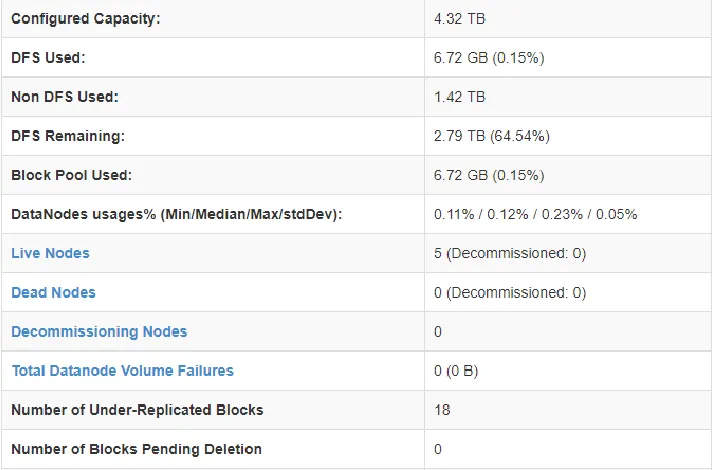
4.1.1 Hadoop

Although Hadoop is not required to run Spark, it was installed because the application

reads data from HDFS. Hadoop was first installed on a single node setting, and then other

nodes were added one at a time. Each time a node was added, the sample MapReduce

tasks were run to make sure that the job was making use of all the nodes. Five nodes

with identical computational power were used to create the cluster. Each node has the

(20)

10

Figure 2:Node CPU configuration

The following table can summarize the final Hadoop configuration:

(21)

11

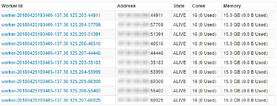
4.1.2 Apache Spark

Apache spark was installed along with SBT and Scala. SBT would be used to build the

Scala projects. Scala was used as the programming language of choice to write streaming

jobs. Spark was installed in the same way as Hadoop by starting with a single node and

adding one node at a time. Two workers instances (SPARK_WORKER_INSTANCES=2)

ran on each terminal to utilize dual CPUs. Each worker was set up to utilize up to 15GB

memory (SPARK_WORKER_MEMORY=15GB) and up to 16 cores

(SPARK_WORKER_CORES=16). Hadoop File System(HDFS) was set up on each of the

nodes. YARN, which works as a resource manager and a dashboard to visualized and

summarize the metrics, was running on the driver node. REPL environment or

Spark-shell was set up in each node to make sure that the debugging would be swift when a

transformation would need to be performed on a set of data. The following figure

(22)

12

Figure 4:Apache Spark Configuration

4.2 Data

4.2.1 Data Files

Data is generated every 6 hours by an oceanographic model (NAVGEM-Navy

Global Environmental Model) that predicts various environmental variables for the next

24 hours to 180 hours. The number of output files from the model depends on the type of

variable. The data is generated for 198 different variables which cover the entire world

with the discreteness of .5 degrees coordinates interval. The model generates multiple

files with the results, and each file only contains data for a single variable which is denoted

(23)

13

only about 4.5 TB disk space available in the distributed file storage, so only four variables

were included for the sake of this experiment. They are ground sea temperature,

pressure, air temperature and wind. Panoply [10] was used a GUI to visualize the input

data and resulting data.

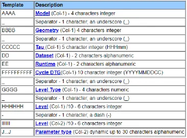
4.2.2 Data Format

The file name for a model result is in the following format:

ProductKey°AAAA_BBBB_CCCCCDDEEFFFFFFFFFF_GGGG_HHHHHH-IIIIIIJ...J

Figure 5:Data file name specifications

This data covers the entire world, so the size of the data array is 361 x 720 where 361

represents all latitude points from -90 degrees north to +90 degrees north with .5 degrees

increments, whereas 720 represents all longitude points from 360 degrees east to 0

(24)

14

4.2.3 Data Collection

Data collection was achieved with various steps. All the steps are defined in the list below:

i. A Java program would download the data into the filesystem. The parameter

type (Part J) in filename above was used to choose the files before

downloading them.

ii. NCAR Command Language was used to convert the data from GRIB format

into the NetCDF3 data format (This changed the variable name by abbreviating

them, so an enum class was written to map the abbreviations with the original

variable names) [11].

iii. CDO (Climate Data Operators - written by the Max Planck Institute for

Meteorology) was used to merge the data files [12]. So, each file could contain

data for multiple variables.

iv. Files were copied to the HDFS using standard HDFS commands.

v. A bash script was written to complete process ii – iv.

4.3 SciSpark

This application extends the functionality of the SciSpark project by changing its open

source code as needed. SciSpark library facilitated the process by mitigating the

necessity to write wrapper classes to represent GRIB. The library provided a class called

SciTensor that represented NetCDF data and implemented all basic mathematical

operations like addition, subtraction, multiplication, etc. [13] New functions were added to

SciTensor class to calculate max, min, and standard deviation. Other significant changes

(25)

15

was added to create unique names for x and y axes when creating NetCDF result file with

more than one variable. RDDs of type SciTensor were created using this library and fed

into the spark streaming queue.

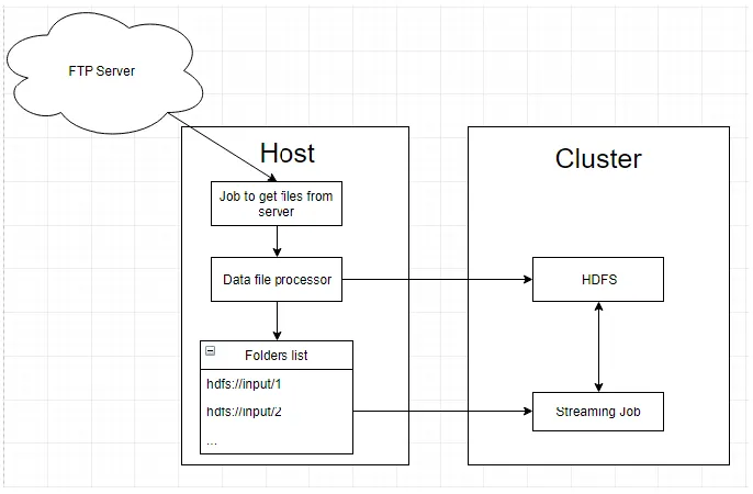
4.4 Application in use

The application streams new files from a location in HDFS and writes the results back to

HDFS. The job runs with a configurable time window and performs transformations and

action on all the RDDs accumulated on that time-frame. QueueStream API in Apache

Spark was used to read the stream of new RDDs inside the streaming job. New RDDs

are represented as a Discretized Stream (DStream) of type SciTensor. Spark Streaming

API defines DStream as a fundamental abstraction in Spark Streaming and is a

continuous sequence of RDDs (of the same type) [14].

The following figure summarizes the outline of the application:

(26)

16

A scheduled job running on the host would run every hour to download new data from the FTP

server. After the download is completed, the data is processed and uploaded to HDFS. The

streaming job running on the cluster would process these new files and update the result. The

website running on a separate server would poll the result file and visualize the data over a Google

(27)

17

Chapter 5

Experiment

Statistical analysis is one of the standard operations that programmers use in Apache

Spark Streaming to generate summary results in real-time. Following properties of a

streaming framework were analyzed:

5.1 Complexity of the operation

This metric would evaluate and measure two significant steps in the streaming process

namely transformation and action. Multiple mathematical queries were designed with a

varying level of complexity and, jobs were run to measure the performance of Apache

Spark Streaming. For example, Average, maximum and minimum are more

straightforward mathematical operation whereas standard deviation can be regarded as

a more complex one. The following statistical analyses were performed:

1. Mean

2. Max

3. Min

4. Standard deviation

Once a user submits the streaming job, it cannot be changed throughout the lifetime of

that job. The input sizes per streaming window for each job were approximately 180MB,

500MB, 1GB, and 2GB. 6 hours streaming window was set for the streaming process

(28)

18

5.1.1 Variation of each Statistical Analysis

Since GRIB1 data represents values in 361 x 720 2D arrays and the values are scattered

across multiple files, to calculate aggregate for each index, same indices across multiple

files were aggregated. To calculate aggregate results for each latitude and longitude

points, 361 and 720 more values in each file needed to be aggregated respectively.

Moreover, calculating one single aggregate result for all the values in all the files

increased the complexity of operation as it had to aggregate more values.

Following list shows the variation in statistical analysis in ascending order of complexity.

1. One result for each combination of latitude and longitude points.

2. One result for each latitude points.

3. One result for each longitude points.

4. One single aggregate result for all data points.

The table below shows the average execution time for each variation of all four-statistical

analysis. It shows that the complexity of operation is directly proportional to the execution

time. More transformations were required on data when running with variation 2, 3 and 4.

Each additional transformation increased the length of the DAG and thus increased the

(29)

19

Variation Dataset Size DAG Length Execution time (s)

1 180MB 5 22

500MB 5 37

1GB 5 49

2GB 5 81

2 180MB 6 23

500MB 6 41

1GB 6 51

2GB 6 101

3 180MB 6 22

500MB 6 43

1GB 6 60

2GB 6 117

4 180MB 7 42

500MB 7 87

1GB 7 133

2GB 7 278

Table 1:Result for statistical analysis

Thus, the performance of a streaming job based on the complexity of the operation was

measured with the different variation of mean, max, min and standard deviation using

GRIB1 data format.

The following code was used to accept a stream of RDDs and run transformations on

them and create the resulting dataset.

val spark = SparkSession .builder

.appName("Multi Variable Spark Streaming") .getOrCreate()

val sc = spark.sparkContext

val convertedVariables: Array[String] = args.map(x => VariableNameMapper.getVariableNameMapping(x))

import org.apache.spark.rdd.RDD

import org.apache.spark.streaming.{Seconds, StreamingContext, Time}

import org.dia.core.{SciSparkContext, SciTensor}

(30)

20

val sssc = new StreamingContext(sc, Seconds(10)) val ssc = new SciSparkContext(sc)

val queue = new mutable.Queue[RDD[SciTensor]]

val scientificRDD = sssc.queueStream(queue) var result: RDD[SciTensor] = null

convertedVariables.foreach(variable => {

val filteredRDD = scientificRDD.filter(p => p != null).map(p=> p(variable)

val meanRDD = filteredRDD.map(x=>x.mean(0)).map(x=>x.mean(1)) val mean = meanRDD.reduce((a, b) => (a + b) / 2)

mean.foreachRDD { (rdd: RDD[SciTensor], time: Time) => if(result == null){

result = rdd }else

{

result = result ++ rdd }

} })

val temp = result.collect().toList temp.foreach(x => {

x.writeToNetCDF("multiVariableMean.nc") })

sssc.start()

5.1.2 Multivariable analysis of the GRIB data

In addition to the metric in section 5.1.1, multivariable analysis was done to measure the

latency of each streaming window. The same four statistical analyses were performed but

with the varying number of variables. These analyses were serialized, thus increasing the

number of transformations and actions for each additional variable. There was 50GB data

(31)

21

process more data. Each streaming window was once again fed with four different

datasets of size 180MB, 500MB, 1GB and 2GB.

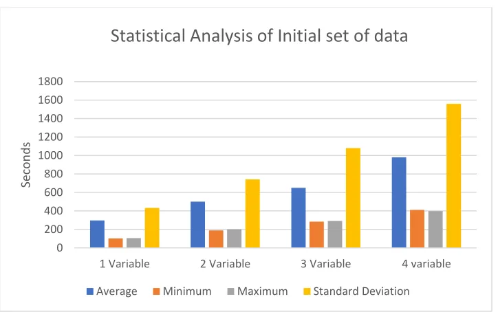
Figure 7:Statistical Analysis of the initial set of data

When the first collect was called, it took a while to generate results. This behavior was

expected as it needed to perform operations on a massive set of data. Also, as expected,

the execution time increased with the complexity of the operation. Standard deviation

took the most amount of time because the algorithm had multiple transformations to be

performed. The following summarizes the algorithm for calculating one standard deviation

for an entire set of data.

Transformation Details

1 Calculate mean for latitudes 2 Calculate mean for longitudes

0 200 400 600 800 1000 1200 1400 1600 1800

1 Variable 2 Variable 3 Variable 4 variable

Se

con

d

s

Statistical Analysis of Initial set of data

(32)

22

3 Calculate the (sum of variance) * (sum of variance) 4 Calculate the sum of variance

5 Calculate the square root of the sum of variance / N Table 2: Standard Deviation and Transformations

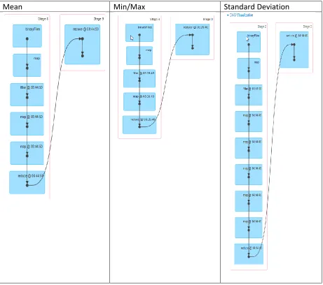
The following table shows the difference in the DAG lengths for mean, min/max, and

standard deviation. It shows that the length of the DAG is directly related to the latency of

the streaming job. In other words, more map and filter functions were run on the dataset,

so each parallel task needed to accomplish more for operations with higher complexity.

Mean Min/Max Standard Deviation

(33)

23

The following chart shows the average time taken for different statistical analysis using

the different number of variables.

Figure 8:Statistical Analysis of batches of stream

Size of the dataset for each 6-hour period was roughly 1GB in size and latency for

streaming 1GB data was significantly smaller than the initial data. For input sources that

generate discrete data at a regular interval, the streaming job is more suitable than a

batch processing job because of the lack of overhead in running an iterative job [15].

5. 2 Number of Executor Nodes

Streaming jobs were run with the different number of worker nodes to record the change

in latency. Data was streamed from HDFS and YARN was used as a dashboard to

visualize states of different worker nodes. Since Apache Spark utilizes the in-memory

datasets [4], the multi-node setup outperformed the single node-setup as it could use

more resource from each worker.

0 200 400 600 800 1000 1200 1400 1600 1800 2000

1 Variable 2 Variable 3 Variable 4 variable

Milli

se

con

d

s

Statistical Analysis of Batches of Stream

(34)

24

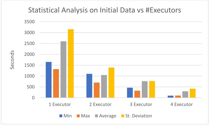
Like the previous metric, the first streaming window had the initial dataset of size 10GB,

so it took longer to process that initial set. It is clear from the chart below that there is

linear scalability regarding latency for a streaming job. Based on the results from this

statistical analysis, one can concur that the efficiency of a streaming job would be directly

proportional to the number of workers.

Figure 9:Statistical analysis on initial Transformation vs. #Executors

On the contrary, if the sample dataset is smaller than the memory used in each worker,

the difference between the efficiency of the streaming jobs are not very significant. So,

we can say that if the dataset is not very big and the initial transformation is not time

sensitive, then even a node cluster would yield similar efficiency. However,

single-node setup comes short on failure recovery as the RDDs would not be replicated across

multiple machines. 0 500 1000 1500 2000 2500 3000 3500

1 Executor 2 Executor 3 Executor 4 Executor

Se

con

d

s

Statistical Analysis on Initial Data vs #Executors

(35)

25

Figure 10:Statistical Analysis of Stream Data vs #Executors

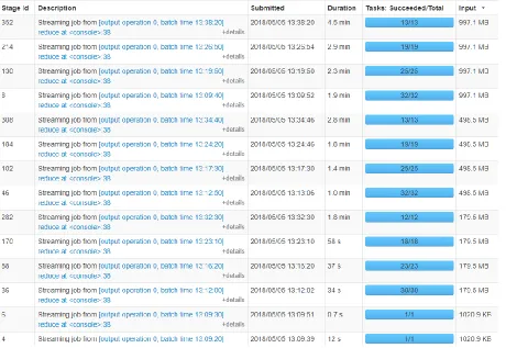
The snapshot below shows the time taken for processing different batches in a

streaming job with the different number of worker nodes.

Figure 11:Streaming jobs ordered by input size for the different number of executors

0 500 1000 1500 2000

1 Executor 2 Executor 3 Executor 4 Executor

Milli

se

con

d

s

Stream Data vs #Executors

(36)

26

In the figure above, stage ids 352, 308, 282 were run with only two executors and 1GB

data, so they took the longest. The lesser number of executors means that each worker

must process a more significant sized chunk of data in parallel as the number of parallel

tasks decreases (this can be seen on tasks: successful/total column in the figure above).

Hence, this increases the overall processing time. If a node has higher processing power,

it can be configured to run higher number of workers. For this experiment, each node was

only configured to run two worker instances.

5.3 Scalability

Another important aspect of any big data processing engine is scalability concerning both

data storage and computational power [16]. As data grows and higher processing speed

is desired, new nodes should be easily added to the cluster. During this experiment,

nodes were killed and started in the cluster with fair speed and easiness. Bash scripts

were written to control the state of a node and YARN dashboard was used to verify the

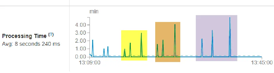
state. Figure 12 shows the state of the cluster after two nodes were killed. Figures 13 and

14 showcase how different metrics of a streaming job can be visualized using apache

spark's dashboard. Figure 13 plots the scheduling delay and figure 14 plots the

processing time for batches ran with the different number of executor nodes. Yellow

represents six executors; brown is five executors and purple is three executors. The sizes

of datasets in different batches were 180MB, 500MB, and 1GB. The scheduling delay

and processing time are both directly proportional to the size of the data and inversely

(37)

27

Figure 12:Showing the status of dead workers on YARN dashboard

Figure 13:Scheduling delay for different dataset with the varying number of executors

(38)

28

5.4 Fault Tolerance

Spark can reconstruct the RDDs using lineage information stored in the RDD objects [4]

when a node falls apart. Since the data is already replicated across nodes in HDFS, lost

partitions can be reconstructed in parallel across multiple nodes without much overhead

[4]. If the node running receiver fails, then another node is spun up with the receiver which

can continue to read from HDFS. If the receiver was using Kafka or Flume as a source

instead of HDFS, then a small amount of data may be lost which hasn't been replicated

to other nodes in the cluster [15]. Performance of a system running streaming job with

various node failures was measured to access the fault tolerance capability of the Apache

Spark Streaming. Spark's dashboard interface was used to visualize the difference in

latency for different batches running with and without node failures. The dashboard also

showed the details about the failure which could aid in debugging the issue during

unexpected failures.

Figure 15:Explanation for a failing node

The figure below shows that if some nodes fail while running a batch, it will take longer to

account for the lost nodes and reschedule those jobs in different node/s. Stage Id 520

lost a node with two workers, and the driver had to reschedule seven tasks running on

(39)

29

(40)

30

Chapter 6

Visual Application

The web interface demonstrates a sample usage of this application. The web page uses

Google Map and its developer API to visualize the results generated by the application.

The web application is written in .NET MVC framework. The server-side code grabs the

latest result from the cluster by using the WinSCP library (this was used to avoid installing

FTP on the master in the cluster), then converts the results into the text format using

ncl_dump. A text dump of the resulting NetCDF file was processed and sent to the view.

A JavaScript function regularly polls for the result, and once the spark application

generates the result, it is visualized on the web.

The following figure summarizes the workflow of the web application:

(41)

31

(42)

32

Following ajax post method is used to poll the cluster to get the latest results.

$.ajax({

type: "POST",

url: "/spark/getdata",

dataType: 'json',

contentType: 'application/json',

success: function (result) {

var reduced = Math.sqrt(259200 / result.data.length);

var response = result.data;

var counter = -1;

removeRectangles();

loop1:

for (var latCounter =

-90; latCounter < 90; latCounter = latCounter + (reduced / 4)) {

for (var longCounter =

-180; longCounter < 180; longCounter = longCounter + reduced) {

counter++;

var value = response[counter];

if (value == undefined) break loop1;

if (latCounter < -86 || latCounter > 84) continue;

var colorcode = "#45CA7B";

if (value < 235) {

colorcode = "#2B9F0E";

} else if (value >= 235 && value < 265) {

colorcode = "#FEFF00";

} else if (value >= 265) {

colorcode = "#FF3F00";

}

var rectangle = new google.maps.Rectangle({

fillColor: colorcode,

fillOpacity: 0.65,

strokeWeight: 0,

map: map,

clickable: false,

bounds: {

north: latCounter,

south: latCounter + (reduced / 4),

east: longCounter + reduced,

west: longCounter

}

});

rectangles.push(rectangle);

}

},

error: function (xhr, status, error) {

$("#errorContainer").append("<div class='alert

alert-danger'>" + error + "</div>");

}

(43)

33

Chapter 7

Findings

7.1 Spark Streaming vs. Hadoop’s batch processing vs. Storm Trident

An iterative job like the one used in this experiment can be expressed as multiple Map

and reduce operations in Hadoop. However, different MapReduce jobs cannot share

data, so for iterative analysis, the same dataset must be read from HDFS multiple times,

and results would need to be written to HDFS many times as well [17]. These iterations

create much overhead because of the I/O operations and other unwanted computations

[18]. Spark tackles these issues by storing intermediate results in the memory. Spark

Streaming uses D-Streams or discretized streams of RDDs which provides consistent,

"exactly-once" processing across the cluster [19] and thus significantly increases the

performance for iterative analysis. Apache Storm can process unbounded streams of data

in real time, and it can be used alongside Hadoop, but it only guarantees "at-least-once"

processing [20]. Trident bolsters Storm by providing micro-batching and other

abstractions that would ensure "exactly-once" processing [21]. It would need three

different libraries to work seamlessly to accomplish what Spark Streaming can

accomplish by itself. Time and effort required to setup and maintain Storm Trident

application along with Hadoop can hamper the production and deployment. On the

contrary, Spark's Streaming library is directly written over its core and maintained by the

same group of people who maintain the core's code base. Thus, spark streaming

(44)

34

7.2 Spark Limitations

The limitation of using Spark over Hadoop boils down to memory. When a dataset is large

enough not to allow any more RDDs to be stored in memory, Sparks starts to replace

RDDs, and such frequent replacement degrades the latency and thus makes Hadoop

more suitable in such situations [22]. When running spark streaming job with two nodes

and four workers with each node getting maximum of 2GB memory, Spark crashed and

threw JVM heap exceptions. So, when memory is not abundant for large datasets, batch

processing in Hadoop is a better choice. However, for this research, we needed a

framework that would seamlessly stream datasets that were only relatively large and

(45)

35

Chapter 8

Related work

H5Spark library could have easily been used in this application instead of SciSpark to

generate RDDs [14]. It takes HDF5 data type as the entry type, and since our data was

in GRIB format, it would have taken two hop conversions from GRIB to NetCDF and

NetCDF to HDF5. The GitHub repo for the H5Spark project consists of streaming

examples, but they were not evaluated for this experiment.

The SciSpark project demonstrates the ability to process NetCDF3/4 data files correctly

and run transformations using Apache spark, but there is no out of the box support for

streaming NetCDF data into the framework [13]. There is an experimental library called

ncstream intended to stream data in GRIB or NetCDF format, and although there isn't any

implementation of using this library in Spark or Hadoop, the possibility for it to be

(46)

36

Chapter 9

Future Work

With the development of new DataFrame API that provides a further abstraction for

creating streaming, graphing or batching jobs in Spark, more sturdy application for

streaming GRIB data can be achieved by refactoring the current logic [25]. For a

long-running streaming job that computes an aggregate like a count or max over a sliding

window, the ReduceByWindow operation can be used [19] [26]. Machine learning libraries

can be used as another metric to compare the iterative data processing with other

frameworks. The same statistical metrics can be run on Storm Trident framework to

compare the latency between the two frameworks. The visualization tool can be extended

(47)

37

Chapter 10

Conclusions

SciSpark was successfully used with Apache Spark to stream GRIB1 data in a streaming

application. The bulk of the logic in this application lies in the ability to convert the

statistical analysis into transformations and actions that would run upon the DStream of

RDDs of type SciTensor. Datasets ranging from 180MB to 50GB were used in the

application without running into any memory issues. Various properties of a streaming

application like operation complexity, scalability and fault tolerance were assessed, and

results were summarized using simple mathematical operations like mean, min/max and

standard deviation. Based on these results and other properties of apache Spark

Streaming, it was deduced that the Spark Streaming is a better solution to stream the

(48)

38

Bibliography

[1] “10 Key Marketing Trends for 2017 and Ideas for Exceeding Customer Expectations.” 10 Key Marketing Trends for 2017, IBM, 19 July 2017, www-01.ibm.com/common/ssi/cgi-bin/ssialias?htmlfid=WRL12345USEN.

[2] Ghemawat, Sanjay, Howard Gobioff, and Shun-Tak Leung. The Google file system. Vol. 37. No. 5. ACM, 2003.

[3] Dean, Jeffrey, and Sanjay Ghemawat. "MapReduce: simplified data processing on large clusters." Communications of the ACM 51.1 (2008): 107-113.

[4] Matei Zaharia, Mosharaf Chowdhury, Michael J. Franklin, Scott Shenker, Ion Stoica, Spark: cluster computing with working sets, Proceedings of the 2nd USENIX conference on Hot topics in cloud computing, p.10-10, June 22-25, 2010, Boston, MA

[5] Gopalani, Satish, and Rohan Arora. "Comparing apache spark and map reduce with performance analysis using k-means." International journal of computer applications 113.1 (2015).

[6] Kroß, Johannes, and Helmut Krcmar. "Modeling and simulating Apache Spark streaming applications." Softwaretechnik-Trends 36.4 (2016): 1-3.

[7] Zaharia, Matei, et al. "Resilient distributed datasets: A fault-tolerant abstraction for

in-memory cluster computing." Proceedings of the 9th USENIX conference on Networked Systems Design and Implementation. USENIX Association, 2012.

[8] Salloum, Salman, et al. "Big data analytics on Apache Spark." International Journal of Data Science and Analytics 1.3-4 (2016): 145-164.

[9] Grulich, Philipp M., and Olaf Zukunft. "Bringing Big Data into the Car: Does it Scale?" Big Data Innovations and Applications (Innovate-Data), 2017 International Conference on. IEEE, 2017.

[10] “Panoply.” NASA, NASA, www.giss.nasa.gov/tools/panoply/.

[11] “Converting GRIB (1 or 2) to NetCDF.” NCL Graphics, Histograms,

www.ncl.ucar.edu/Applications/griball.shtml.

[12] Schulzweida, U., L. Kornblueh, and R. Quast. "CDO User’s Guide: Climate Data Operators Ver. 1.6. 1."

[13] Palamuttam, Rahul, et al. "SciSpark: Applying in-memory distributed computing to weather event detection and tracking." 2015 IEEE International Conference on Big Data (Big Data). IEEE, 2015.

[14] Zaharia, Matei, et al. "Apache spark: a unified engine for big data processing." Communications of the ACM 59.11 (2016): 56-65.

(49)

39

[16] Murray, Derek G., et al. "Naiad: a timely dataflow system." Proceedings of the Twenty-Fourth ACM Symposium on Operating Systems Principles. ACM, 2013.

[17] Bu, Yingyi, et al. "HaLoop: efficient iterative data processing on large clusters." Proceedings of the VLDB Endowment 3.1-2 (2010): 285-296.

[18] Ekanayake, Jaliya, et al. "Twister: a runtime for iterative mapreduce." Proceedings of the 19th ACM international symposium on high performance distributed computing. ACM, 2010.

[19] Zaharia, Matei, et al. "Discretized streams: Fault-tolerant streaming computation at scale." Proceedings of the Twenty-Fourth ACM Symposium on Operating Systems Principles. ACM, 2013.

[20] Toshniwal, Ankit, et al. "Storm@ twitter." Proceedings of the 2014 ACM SIGMOD international conference on Management of data. ACM, 2014.

[21] Apache Storm. (2014, December) Trident Tutorial. [Online].

https://storm.apache.org/documentation/Tridenttutorial.html

[22] Gu, Lei, and Huan Li. "Memory or time: Performance evaluation for iterative operation on hadoop and spark." High Performance Computing and Communications & 2013 IEEE

International Conference on Embedded and Ubiquitous Computing (HPCC_EUC), 2013 IEEE 10th International Conference on. IEEE, 2013.

[23]Liu, Jialin, et al. "H5spark: bridging the I/O gap between spark and scientific data formats on Hpc systems." Cray user group (2016).

[24] “NetCDF Streaming Format (Experimental).” Ncstream, 1 Nov. 2010,

www.unidata.ucar.edu/software/thredds/v4.3/netcdf-java/stream/NcStream.html

[25] Armbrust, Michael, et al. "Scaling spark in the real world: performance and usability." Proceedings of the VLDB Endowment 8.12 (2015): 1840-1843.

(50)

40

Vita

The author Janak Dahal was born in Tehrathum, Nepal. He received his Bachelor's

Degree in Computer Science from the University of New Orleans in 2012. After three

years of professional work, he joined Graduate program of Computer Science at The

University of New Orleans. He worked at Canizaro Livingston Gulf States Center for

Environmental Informatics center as a graduate assistant while working on his Thesis.

This research work was conducted under the supervision of Dr. Mahdi Abdelguerfi and

Assessing Apache Spark Streaming with Scientific Data

ScholarWorks@UNO

ScholarWorks@UNO

Assessing Apache Spark Streaming with Scientific Data

Assessing Apache Spark Streaming with Scientific Data

Acknowledgments

Contents

List of Figures

List of Tables

Abbreviations

Abstract

Chapter 1

Introduction

Chapter 2

Background

Chapter 3

Apache Spark

3. 1 Resilient Distributed Data (RDD)

3.1.1 Replicated

3.1.2 Immutable

3.1.3 Resilient

3.2 Apache Spark Streaming

Chapter 4

Application

4.1 Setup

4.2 Data

4.3 SciSpark

4.4 Application in use

Chapter 5

Experiment

5.1 Complexity of the operation

Statistical Analysis of Initial set of data

5. 2 Number of Executor Nodes

Statistical Analysis of Batches of Stream

Statistical Analysis on Initial Data vs #Executors

Stream Data vs #Executors

5.3 Scalability

5.4 Fault Tolerance

Chapter 6

Visual Application

Chapter 7

Findings

7.1 Spark Streaming vs. Hadoop’s batch processing vs. Storm Trident

7.2 Spark Limitations

Chapter 8

Related work

Chapter 9

Future Work

Chapter 10

Conclusions

Bibliography

Vita