* Corresponding author.
E-mail: [email protected] (M. Mutingi) © 2013 Growing Science Ltd. All rights reserved. doi: 10.5267/j.ijiec.2013.01.003
International Journal of Industrial Engineering Computations 4 (2013)177–190
Contents lists available at GrowingScience
International Journal of Industrial Engineering Computations
homepage: www.GrowingScience.com/ijiec
A fuzzy simulated evolution algorithm for integrated manufacturing system design
Michael Mutingi*
Mechanical Engineering Department, University of Botswana, P Bag UB 0061, Botswana
C H R O N I C L E A B S T R A C T
Article history:
Received September202012 Received in revised format December 28 2012
Accepted January2 2013 Available online 3January 2013
Integrated cell formation and layout (CFLP) is an extended application of the group technology philosophy in which machine cells and cell layout are addressed simultaneously. The aim of this technological innovation is to improve both productivity and flexibility in modern manufacturing industry. However, due to its combinatorial complexity, the cell formation and layout problem is best solved by heuristic and metaheuristic approaches. As CFLP is prevalent in manufacturing industry, developing robust and efficient solution methods for the problem is imperative. This study seeks to develop a fuzzy simulated evolution algorithm (FSEA) that integrates fuzzy-set theoretic concepts and the philosophy of constructive perturbation and evolution. Deriving from the classical simulated evolution algorithm, the search efficiency of the major phases of the algorithm is enhanced, including initialization, evaluation, selection and reconstruction. Illustrative computational experiments based on existing problem instances from the literature demonstrate the utility and the strength of the FSEA algorithm developed in this study. It is anticipated in this study that the application of the algorithm can be extended to other complex combinatorial problems in industry.
© 2013 Growing Science Ltd. All rights reserved Keywords:
Integrated cell formation and layout (CFLP)
Fuzzy simulated evolution algorithm (FSEA) Metaheuristic
1. Introduction
overall process of designing cellular manufacturing system involves the following three critical generic decisions:
1. Cell formation: involves grouping of machines which can operate on a product family with little or no inter-cell movement of the products.
2. Group layout: includes layout machine within each cell (intra-cell layout), and layout of cells with respect to one another (inter-cell layout).
3. Group scheduling: this involves scheduling of parts for production
In respect of the above, the most ideal situation is that these criteria should be addressed concurrently, if the advantages of cellular manufacturing system design are to be fully realised (Kaebernick&Bazargan-Lari, 1996; Mahdavi&Mahadevan, 2008; Jayaswal&Adil, 2004.). Nevertheless, the CFLP is a complex combinatorial problem that is difficult to solve using conventional approaches. As such, most of the cell formation studies have focused on these decisions independently or sequentially, resulting in loss of quality solutions (Selim, 1998; Onwubolu&Mutingi, 2001).
In most cellular manufacturing system design problems in the literature, researchers and layout designers used sequence data (flow patterns of parts) for cell design issues only. On the other hand, the layout designers did not consider the cell formation problem (CFP) at all. Since sequential approaches address the cell formation and the cell layout problem in a sequential disjointed fashion, the quality of the final solution is compromised. The current study presents an integrated approach to cell formation and layout design based on use of available sequence data. Fuzzy set theory is used to develop fuzzy evaluation criteria for the CFLP problem. The fuzzy evaluation concepts are incorporated into simulated evolution algorithm (SEA) in order to develop an enhanced fuzzy simulated evolution algorithm (FSEA). The FSEA approach utilizes sequence data to identify machine cells as well as machine layout within each cell. In this vein, the specific objectives for this research are outlined as follows:
1) to develop relevant performance metrics to address the integrated cell formation and layout
problem.
2) to develop enhanced fuzzy evaluation criteria for the CFLP, based on the concepts of fuzzy
theory;
3) to develop a FSEA algorithm that incorporates the proposed fuzzy evaluation criteria; and, 4) to carry out illustrative computational experiments based on data sets in the CFLP literature. The advantages of the proposed FSEA approach include the following: (i) the algorithm mimics iterative evolution on a single solution, which considerably eliminates extra CPU time; (ii) the FSEA, unlike genetic algorithms, selects and discards inferior cells of only one solution in accordance with the goodness of each cell, and (iii) the algorithm has strong convergence capabilities leading to fewer iterations when compared to other competitive evolutionary metaheuristics. The strength of the algorithm is demonstrated on problem sets in the literature.
The remainder of the paper is structured as follows. Section 2 explores related work in the literature, covering the CFLP problem, metaheuristics, simulated evolution algorithm, and fuzzy theory. Section 3 gives an outline of the proposed FSEA algorithm, describing the related operators. Computational tests, results and relevant discussions are presented in Section 4. Finally, conclusion and further research are provided in Section 5.
2. Related work
metaheuristic algorithms. A typical example of hard combinatorial problem is the integrated cell formation and layout problem (CFLP).
2.1 The CFLP problem
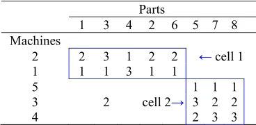
The integrated cell formation problem is a new joint approach to cell formation and layout problem that seeks to identify manufacturing cells and the layout (sequence) of machines in the cells in an integrated manner. The whole aim of the approach is to avoid compromising the quality of solutions with respect cell formation and cell layout objectives. Therefore, this approach to the joint layout problem is of practical value. The basic CFP is NP-complete, meaning that it has no known polynomial time algorithm due to its combinatorial nature (Kumar et al., 1986). It follows that the integrated cell formation and cell layout problem is highly computationally intractable. In solving the CFLP, typical objective functions include (i) minimization of inter-cell movements, (ii) minimization of intra-cell movements, (iii) minimizing cell work-load imbalances and (iv) minimization of material handling costs. Fig. 1 provides an example of a typical solution to an 8 part × 5 machine cell formation problem in which cell 1 (machines 2 and 1) manufactures parts 1, 3, 4, 2 and 6, and cell 2 (machines 5, 3, and 4) manufactures parts 5, 7 and 8. The sequence data represents the flow of parts between machines, for example, part 1 (in cell 1) flows from machine 1 to machine 2, and part 3 flows from machine 1 to 3 and finally to machine 2. Thus, the facility planner considers 2 possible cell 1 layout, that is (1-2) or (2-1). The CFLP considers that, apart from cell formation, intra-cell layout should be considered as well.
Parts 1 3 4 2 6 5 7 8 Machines
2 2 3 1 2 2 ←cell 1
1 1 1 3 1 1
5 1 1 1
3 2 cell 2→ 3 2 2
4 2 3 3
Fig. 1. A solution to an 8×5 cell formation problem
2.2 Metaheuristic approaches
Metaheuristics such as simulated annealing (SA), genetic algorithms (GA), and evolutionary algorithms (EA) are potential intelligent algorithms that can obtain near-optimal solutions to hard problems such as the CFLP problem. SA is a stochastic optimization technique based on an analogy from statistical mechanics, in which a substance is reduced to its lowest energy configuration by a sequence of steps that involve alternate heating and cooling. On the other hand, GA is a population-based search and optimization algorithm derived from the principles of evolution and survival of the fittest (Goldberg, 1989). It uses the mechanics of stochastic genetic operators such as crossover and mutation to guide its search and optimization process towards regions of the search space with likely improvement.
Furthermore, EA is a population-based metaheuristic optimization algorithm inspired by the
mechanisms of biological evolution, such as reproduction, mutation, recombination, and selection. Candidate solutions evolve through generations after repeated applications of the naturally-inspired operators. Simulated evolution algorithm (SEA), like EA, is a potential evolutionary algorithm for solving large-scale cell formation and layout problems.
2.3 Simulated evolution algorithm
prove its effectiveness (fitness) under current conditions in order to remain intact so as to proceed to the next generation. The end goal is to gradually create stable structures, perfectly adapted to the given constraints. To escape from local optima, a genetic mutation operator is used for the perturbation of genetic inheritance (Ly &Mowchenko, 1993).
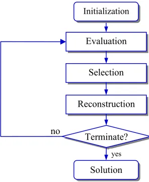
Basically, the SEA algorithm is an iterative algorithm that consists of a sequence of operators, namely:
evaluation, selection and reconstruction, operating on one candidate solution (Saiti et al., 1999) as shown in Fig. 2. Prior to the aforementioned operators, some critical input parameters and a valid starting solution are initialised in the initial step known as initialization. In evaluation, the fitness of each element in the current solution is computed in accordance with the objective of the optimization process. In this connection, a goodness measure is used to probabilistically select elements to be discarded during the selection stage; an element with high goodness has a lower probability of being discarded. The resulting partial solution is then fed to the reconstruction operator that implements specific heuristics to repair and derive a new and complete solution from the partial solution.
In the SEA iteration process, the best solution is always preserved and finally returned as the solution to the problem (Saiti& Ismail, 2004; Li & Kwan, 2002). Thus, the basic SEA algorithm is a search heuristic that achieves improvement through iterative perturbation and reconstruction. However, to enhance its evaluation, selection, mutation and reconstruction processes, the basic SEA needs to incorporate fuzzy theory concepts so as to increase its search and optimization efficiency.
Fig. 2. Simulated evolution algorithm
2.4. Fuzzy set theory
Fuzzy set theory, introduced by Zadeh (1965) as a means of presenting uncertainty, has been developed further to provide a flexible and robust methodology to address and solve complex real-world problems (Dubois &Prade, 1980). The concepts of fuzzy theory can be understood best when explained by contrasting fuzzy sets and crisp sets.
Definition 1:Classical crisp set. Let X be the universe of objects having elementsx, and let A denote a proper subset of the universe X. Then, the membership of x in a classical crisp set A can be viewed as a characteristic transformation function μA from X to {0,1}, such that,
1 If ( )
0 If A
x A x
x A
μ = ⎨⎧ ∈
∉ ⎩
(1)
Evaluation
Selection
Reconstruction
Terminate?
yes no
Initialization
Definition 2:Fuzzy set. A fuzzy set an be described as follows: For a fuzzy set A of the universe X, the grade of membership of x in A can be defined as μA(x)∈[0,1], where μA(x) is the membership function whose value ranges from 0 to 1.
According to definition 2, the fuzzy set A has no sharp boundary; the closer the value of μA(x) is to 1, the more x is said to belong to A. Contrary to the crisp set, each of the subsets of Xcan be shown to have a one-to-one correspondence with the characteristic function. Retrospectively, since the membership function is an extension of the characteristic function, fuzzy sets are extensions of crisp sets. The cells of a fuzzy set are ordered pairs that reflect the value of each cell in the set and its grade of membership as in the expression;
(
)
{
, A( ) |}
A= x μ x x X∈ (2)
3. Fuzzy simulated evolution algorithm
The FSEA algorithm incorporates the concepts of fuzzy theory into the classical SEA. In this regard, the SEA stages, that is, initialization, evaluation and reconstruction, are fuzzified. The proposed fuzzy simulated evolution algorithm and its major components are described in this section. Some key definitions and terminologies need to be clarified in order to facilitate the discussions that follow.
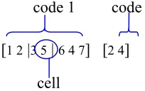
Definition 3: Solution space. Let C = {C1, C2,...,Cm} denote a set of all possible cells (cells) for the CFLP problem, where m is the number of cells. Then C is a solution space consisting of all possible cells. Each cell consists of machines (items).
Definition 4: Candidate solution. A candidate solution S* is defined as the most suitable combination of cells at the current iteration. This implies that S*⊆C.
In view of the above definitions, a typical candidate solution to the CFLP is coded in form of cells that consist of machines. Fig. 3 provides a candidate solution for a typical problem where 6 machines are to be grouped into 3 cells; each cell must have a minimum of 2 machines, and inter-cell movements are to be minimized. The current candidate solution, coded as [1 2 | 3 5 | 6 4 7] in code 1, is made up of machine cells (1-2), (3-5), and (6-4-7). Code 1 defines the part of the solution upon which the operators of the algorithm acts. On the other hand, code 2 basically defines the position of the delimiters (“|”) that separate the cells in the solution.
code 1 code 2
[1 2 |3 5 | 6 4 7] [2 4]
cell
Fig. 3. Candidate solution representation
3.1 Initialization phase
defined in terms of (i) predetermined number of iteration specified by the user, or (ii) the maximum allowable number of iterations without solution improvement.
3.2 Evaluation phase
Fuzzy evaluation is the first step of the iterative loop where a goodness of fit (fitness) is determined for the structure of each cell in the solution S*. The main purpose of evaluation phases is to determine the overall contribution of each cell to the solution fitness, and to determine which cells contribute much less than acceptable. Poorly performing cells are discarded, however, with a probability. The fuzzy evaluation for a typical CFLP solution S* , comprising m cells, is achieved by first defining the fitness of each cell c (c = 1,2,...,m) in terms of a membership function μ1which measures the goodness of each
cell according to the following expression;
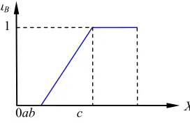
Definition 5:Trapezoidal fuzzy number. A trapezoidal fuzzy number B, illustrated in Fig.4, is defined by the membership function μB:X→[0,1] as shown by expression;
(
) (
)
1 if
( ) if a
0 if otherwise B
x b x x a b a x b
μ
≥ ⎧
⎪
=⎨ − − ≤ ≤
⎪ ⎩
(3)
where, b is the most preferred value, and a and c are the lower and upper bounds of the fitness function values, respectively.
Fig. 4. Trapezoidal fuzzy membership function
The fitness of each cell c in the current solution S* is computed based on a fuzzy membership function
F(c), which is a combination of normalized fuzzy functions. This implies that for a CFLP consisting of
n evaluation functions, f1, f2,..., fn, the overall evaluation function F(c) for cell c can be computed as follows:
* 1
( ) n i( ) i
F c f c c S =
=
∏
∀ ∈ (4)where, n is the number of evaluation functions, c denotes the cell in the current solution S*.
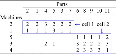
From the CFP design perspective, the existence of voids and exceptions should be minimized as much as possible. In layout design, the key consideration is adjacency of machines in a cell is a as it can reduce material handling costs significantly (Mahdavi et al., 2010). From a production planning and control perspective, the machines sequence inside the cells may potentially create unwanted reverse flows and skipping of workstations. For example, referring to Fig. 5, cell 1 has two possible machine sequences (layouts), that is, (1-2) or (2-1). Cell layout (1-2) has only 4 consecutive forward flows,
1
μB
X c
while (2-1) has only 1; thus, from this analysis, layout (1-2) is preferred. In the same way, layout (5-3-4) is chosen as the best layout for cell 2.
Parts
2 1 4 5 3 7 6 8 9 10 11
Machines
2 2 2 3 2 2 2 ←cell 1 cell 2
1 1 1 1 3 1 1 ↓
5 1 1 1 1 2
3 2 1 3 2 2 2 3
4 2 3 3 3 1
Fig. 5. A typical solution for a cell formation problem
Ideally, a good objective function should not only solve the cell formation problem, but also should also evaluate the effects of machine sequence (layout) within each cell. A simplified way of evaluating the fitness of a cell layout is to express the objective function in terms of the number of consecutive forward flows. In this vein, Mahdavi and Mahadevan (2008) defined the cell flow index (CFI) and the overall flow index (OFI) for evaluating the cell design and layout. We use the following notation in this model.
Notation:
n number of parts in the system
m number of machines in the system
nc number of parts in cell c
mc number of machines in cell c
vc number of voids in cell c
Nfc number of consecutive forward flows within cell c
Nec number of exceptional flows due to parts assigned to cell c
S [sjk] machine-component incidence matrix in terms of sequence data, sjk= 0 if part j does not visit machine k; sjk = 0 otherwise
To define the average flow and overall flow performance measures, the total number of operations and the consecutive flows between a pair of machines are calculated. The total number of flows Nflowis
defined as follows:
max flow j jk
k
N =
∑
s −n (5)The total number of flows Ntc within each cell c is determined according to the following expression:
( )
tc c c c c
N = n m − −v n (6)
3.2.1 Cell flow index (CFI)
The cell flow index for cell c, CFIc is the ratio of the number of consecutive forward flows to the total
number of flows within the cell. The cell average flow index is the weighted average of CFIs, as shown by the following expressions;
c CFI fc
tc
N N
= (7)
the solution quality with respect to the number of voids and the intra-cell moves. Overall, we define the average cell flow index (ACFI) to measure the overall performance of the manufacturing system, that is;
c
1
ACFI cCFI
c n n ⎛ ⎞
=⎜ ⎟⋅
⎝ ⎠
∑
(8)
3.2.2 Inter-cell flow index (IFI)
The inter-cell flow index defines the ratio of the number of flows due to exceptional parts in cell c and the number of flows in cell c. This can be represented by the following expression;
c
IFI tc tc ec
N N N
= +
(9)
At system level, we utilize the overall cell flow index (OFI), which defines the ratio of the sum of consecutive forward flows in all the cells to the total number of the flows required to process all the parts (Mahdavi&Mahadevan, 2008). Decreasing the values of inter-cell moves will increase the values of OFI. The OFI defines the extent of inter-cell moves (exceptions) for the manufacturing system as follows;
1
OFI fc
c flow
N N
⎛ ⎞
=⎜⎜ ⎟⎟⋅
⎝ ⎠
∑
(10)
While the OFI points to the inter-cell movements, the ACFI addresses the intra-cell movements. Consequently, a combination of these performance measures ensures that the cell formation and layout are addressed jointly. Since the focus of this application is on the use of CFIc and IFIc in the evaluation
stage, these indices are combined according to expression (4) to obtain fitness function F. The ACFI and OFI are merely utilized for the overall evaluation of the overall candidate solution to the CFLP.
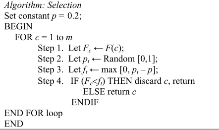
3.3 Selection
The purpose of the selection stage is to probabilistically determine whether or not an cell c in solution
S*should be retained for the next generation. The selection procedure ensures that a cell c with a high fitness value Fc = F(c) has a higher probability of surviving into the next iteration. However, if not retained, the cell is placed in a queue for the next allocation phase. The selection process is achieved by comparing the fitness F(c) of each cell c with a predetermined allowable fitness ft defined at iteration t;
max[0, ]
t t
f = p −p (11)
where, pt is a random number in the range [0,1] at iteration t; p is a predetermined constant less than 1. In connection with the above, we generalize the selection procedure according to the algorithm shown in Fig. 6.
Algorithm: Selection Set constant p = 0.2; BEGIN
FOR c = 1 to m
Step 1. Let Fc ←F(c); Step 2. Let pt ← Random [0,1]; Step 3. Let ft ← max [0, pt – p];
Step 4. IF (Fc<ft) THEN discard c, return ELSE return c
ENDIF END FOR loop
END
The discarded cell are set aside to be considered in the next reconstruction phase. The expression ft
=pt– p enhances the algorithm’s convergence ability. When the value of pt is high, the probability of discarding good cells are very high, which leads to inefficiency. Thus, by setting the value of p to a reasonable value (e.g., p = 0.2), the search power can be controlled effectively.
3.4 Mutation
Mutation is useful for intensification and exploration. Whereas intensification facilitates local search around the current best solution S*, exploration enables the algorithm to explore unvisited regions of the solution space. The two search procedures, that is, intensification and exploration, are utilized in this phase. Intensification is achieved through swapping of randomly chosen pairs of machines within a single cell. This mutation mechanism avoids generation of infeasible solutions, and enhances the computation speed of the algorithm. On the other hand, explorative mutation is an evolutionary mechanism by which FSEA moves from local optima. This is achieved by probabilistically eliminating some cells of the solution, even the best performing ones. In this respect, each cell Ej has a chance to be randomly eliminated from the partial solution. In general the mutation operation is applied at a very
low probability pm, so as to ensure convergence. In this application, we use a decay function to
formulate a dynamic mutation probability as follows;
1 0 ( ) i I m
p i =p e− (12)
wherei is the iteration count; I is the maximum allowable number of iterations; and p0 is the initial
mutation probability. The formulation of pm(i) can be used for both explorative and intensive mutation probabilities. It is important to note that during explorative mutation, infeasible partial solutions may be created. However, these solutions will be repaired in the reconstruction phase.
3.5 Reconstruction
The reconstruction phase is concerned with re-building a partial solution which evolved from the previous phases into a complete solution. This implies that all the cells and their assigned machines should remain unchanged. Therefore, the reconstruction phase essentially deals with the assignment of machines to empty spaces in every incomplete cell. Thus, this is achieved through the use of repair mechanisms specially designed in consideration of the context of the CFLP problem. In every reconstruction phase, a number of combinations of machines and cells are possible. We build an effective reconstruction procedure by using a greed-based heuristic that assumes that the attractiveness of adding a cell c into the current incomplete solution increases with its fitness function value F(Sj). As such, the algorithm keeps a limited candidate list (CL) of best performing cells, comprising k cells. A suitable value of kis chosen through experimentation. From the illustrative experiments carried out in this study, the best values of k are such that, k≤ 0.3N, where N is the maximum permissible number of cells. The general structure of the reconstruction procedure is illustrated in Fig. 7.
Algorithm: Reconstruction BEGIN
Step 1. Let S* = {1,2,..., s} denote a partial solution, where, s is the index for each cell;
Step 2. Set CL= N best cells from S, based on F(c); Step3. Set ( *: )
∗
∗∈
− =
′ I E j S
I ∪ j where I is a set of all machines; Step 4. IF (I′ = φ) THEN stop, return S*; S* is a complete solution; ELSE randomly select a cellcr∈CL
ENDIF;
Step 5. Add cr to S*, set I′ - cr, and return to Step 4. END
It is important to note that in some cases the reconstruction algorithm may generate redundant machines. In other words, some machines will be repeated, and, consequently, some will be missing. This implies that the current solution needs to go through a self-correction mechanism, called reconfiguration. First, two sets of repeated and missing machines are identified. Second, repeated machines are replaced with the identified missing machines, such that the solution is transfigured to a feasible solution. The general algorithm for the reconfiguration process is shown in Fig. 8.The next section provides computational experiments, results and relevant discussions based on benchmark problem sets from the literature.
Algorithm: Reconfiguration BEGIN
Step 1. Set R1={1,2,...,r1}a set of repeated machines in S *;
Step 2. Set R2 ={1,2,...,r2}a set of missing machines in S *; Step 3. Replace R1 with R2 machines in S*
END
Fig. 8. Algorithm for the reconfiguration procedure
4. Computational tests and results
In order to assess the effectiveness of the FSEA approach, the algorithm is tested on typical CFLP problems in the literature. Thus, numerical illustrations were performed based on data sets obtained data sets obtained from the literature (Nair &Narendra, 1998; Harhalakis et al., 1990; Tam, 1988).
4.1 Computationalillustrations
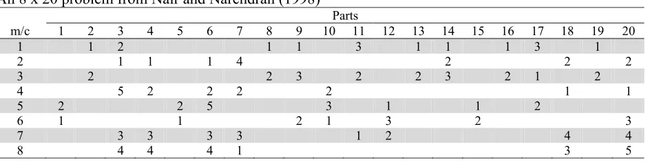
The overall objective functions, ACFI and OFI, were used as the overall performance value of the solutions. Illustrative computations were carried out based on an 8 × 20 problem obtained from Nair and Narendran (1998), as shown in Table 1.
Table 1
An 8 x 20 problem from Nair and Narendran (1998)
Parts m/c 1 2 3 4 5 6 7 8 9 10 11 12 13 14 15 16 17 18 19 20
1 1 2 1 1 3 1 1 1 3 1
2 1 1 1 4 2 2 2
3 2 2 3 2 2 3 2 1 2
4 5 2 2 2 2 1 1
5 2 2 5 3 1 1 2
6 1 1 2 1 3 2 3
7 3 3 3 3 1 2 4 4
8 4 4 4 1 3 5
Table 2
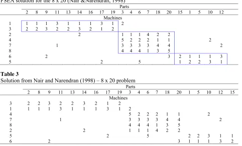
FSEA solution for the 8 x 20 (Nair &Narendran, 1998)
Parts 2 8 9 11 13 14 16 17 19 3 4 6 7 18 20 15 1 5 10 12
Machines
1 1 1 1 3 1 1 1 3 1 2
3 2 2 3 2 2 3 2 1 2
2 2 1 1 1 4 2 2
4 5 2 2 2 1 1 2
7 1 3 3 3 3 4 4 2
8 4 4 4 1 3 5
6 2 3 2 1 1 1 3
5 2 5 1 2 2 3 1
Table 3
Solution from Nair and Narendran (1998) – 8 x 20 problem
Parts 2 8 9 11 13 14 16 17 19 3 4 6 7 18 20 1 5 10 12 15
Machines
3 2 2 3 2 2 3 2 1 2
1 1 1 1 3 1 1 1 3 1 2
4 5 2 2 2 1 1 2
7 1 3 3 3 3 4 4 2
8 4 4 4 1 3 5
2 2 1 1 1 4 2 2
5 2 5 2 2 3 1 1
6 2 3 1 1 1 3 2
4.2 Comparative experiments
To illustrate the utility of the proposed FSEA algorithm, a comparative study was done considering FSEA, CASE and CLASS algorithms. Table 4 provides the results of the comparative study. Though machine groups and part families are the same for the three algorithms, the ACFI and OFI differ with CASE solution. However, the ACFI and OFI values of FSEA are similar to those obtained from CLASS. This shows the remarkable improvement of the solution to the joint cell formation and layout problem.
Table 4
Comparative study of FSEA, CASE and CLASS algorithms - 8 x 20 problem
Cell
No. CASE Solution CLASS Solution FSEA Solution
nc Nfc Ntc CFI% nc Nfc Ntc CFI% nc Nfc Ntc CFI% 1 9 1 9 11.1 9 5 9 55.6 9 5 9 55.6
2 6 7 18 38.9 6 9 18 50 6 9 18 50
3 5 1 5 20.0 5 2 5 40.0 5 2 5 40.0 Nflow = 41
ACFI (%) 21.0 50.0 50.0
OFI (%) 22.0 39.0 39.0
Table 5
Comparison of FSEA with other algorithms
Data Set
Size CLASS Fuzzy Art Hierarchical FSEA
Cells ACFI OFI Cells ACFI OFI Cells ACFI OFI Cells ACFI OFI 1. 12 × 19 2 65% 50% 2 49% 36% 2 48% 45% 2 65% 50% 2. 20 × 20 4 65% 41% 4 42% 34% 4 42% 34% 4 69% 43% 3. 25 × 40 4 52% 34% 7 38% 27% 8 37% 22% 4 68% 42% 4. 08 × 20 3 50% 39% - - - - - - 3 50% 39% Key: 1. Tam (1988); 2. Harhalakis et al. (1990); 3. Nair &Narendra (1998); 4. Nair &Narendra (1998)
The results obtained in this comparative study are shown in Table 6. In all cases, the ACFI and OFI values obtained by FSEA are much more preferable than those obtained from other algorithms. From this analysis, it can be seen that the utilization of sequence data in joint cell design and layout is important.
5. Conclusions and further research
The integrated cell formation and layout problem is a complex combinatorial problem common in advanced manufacturing systems. The use of sequence data in solving CFLP provides valuable additional information on the dominant flow patterns, which provides a platform for solving the problem. The challenge is on how to extend the application of sequence data and to develop a robust algorithm for solving the joint design and layout problem. In this study, a FSEA was proposed to solve the integrated design and layout problem based on sequence data. The approach incorporates into the well known simulated evolution algorithm the concepts of fuzzy set theory, including iterative improvement and constructive perturbation so as to improve the optimization and search capability of the algorithm.
Computational results based on a set of benchmark problems concerned with the cell formation problem from the literature revealed that FSEA is a competitive algorithm which can solve hard combinatorial problems. A number of advantages of the FSEA are realised in this research. First, the algorithm is easy to conceptualize, construct and computerize. Second, unlike other competitive algorithms such as genetic algorithms, FSEA works on a single candidate solution, rather than on a population of solutions. The algorithm iteratively eliminates less performing cells, unlike other meta-heuristics such as simulated annealing. This enhances FSEA convergence ability; hence, the algorithm can obtain a good solution within a shorter computation time. Third, FSEA is characterized with features of probabilistic hill climbing that provide the algorithm with the power to explore unvisited regions of the solution space.
Possible future research directions include the application of the FSEA to other hard combinatorial problems such as production scheduling, aggregate production planning, and workforce scheduling. Improving the efficiency and effectiveness of the FSEA algorithm is another area of focus.
References
Aryanezhad, M. B., Aliabadi, J., & Tavakkoli-Moghaddam, R. (2011). A new approach for cell formation and scheduling with assembly operations and product structure. International Journal of Industrial Engineering Computations, 2(3), 533-546.
Dubois, D., & Prade, H. (1980). Fuzzy Sets and Systems: Theory and Applications. Academic Press, New York.
Forghani, K., Khamseh, A. A., &Mohammadi, M. (2012).Integrated quadratic assignment and continuous facility layout problem.International Journal of Industrial Engineering Computations, 3(5), 787-806.
Ghezavati, V. R. (2011). A new stochastic mixed integer programming to design integrated cellular
manufacturing system: A supply chain framework. International Journal of Industrial Engineering
Computations, 2(3), 563-574.
Goldberg, D.E. (1989). Genetic Algorithm in Search, Optimization, and Machine Learning’,
Addison-Wesley, Reading, MA.
Ghosh, T., Sengupta, S., Chattopadhyay, M., & Dan, P. K. (2011). Meta-heuristics in cellular
manufacturing: A state-of-the-art review. International Journal of Industrial Engineering
Computations, 2(1), 87-122.
Hamedi, M., Ismail, N., Esmaeilian, G. R., &Ariffin, M. K. A. (2012).Virtual cellular manufacturing system based on resource element approach and analyzing its performance over different basic layouts.International Journal of Industrial EngineeringComputations, 3(2), 265-276.
Harhalakis, G. Nagi, R., &Proth J.M. (1990).An efficient heuristic in manufacturing cell formation for group technology applications.International Journal of Production Research, 28, 185-198.
Jayaswal, S. and Adil, G. K. ( 2004). Efficient algorithm for cell formation with sequence data, machine replications and alternative process routings.International Journal of Production Research, 42, 2419-2433.
Kling, R.M., &Banejee, P. (1987). ESP: A New Standard Cell Placement Package Using Simulated
Evolution. Proceedings of the 24th ACWIEEE Design Automation Conference, 60-66.
Li, J., & Kwan, R.S.K. (2002). A fuzzy evolutionary approach with Taguchi parameter setting for the
set covering problem. Proceedings of the 2002 IEEE Congress on Evolutionary Computation,
1203-1208.
Lin, Y.L., Hsu, Y.-C., & Tsai, F.S. (1989). SILK: A Simulated Evolution Router. IEEE Transaction on Computer-Aided Design, 8, 1108-1114.
Ly, T.A. &Mowchenko, J.T. (1993). Applying Simulated Evolution to High Level Synthesis. IEEE
Transaction on Computer-Aided Design of Integrated Circuits and Systems, 12, 389-409.
Mahdavi, I. &Mahadevan, B. (2008). CLASS: An algorithm for cellular manufacturing system and layout design using sequence data. Robotics and Computer-Integrated Manufacturing, 24, 488-497. Mahdavi, M. I., Tahami, B. N., Teymourian, E. (2010). A new cell formation problem with the
consideration of multifunctional machines and in-route machines dissimilarity - A two phase
solution approach.IEEE 17th International Conference on Industrial Engineering and Engineering
Management, 2010, 475-479.
Mutingi, M. & Mbohwa, C., Mhlanga, S., & Goriwondo, W. (2012). Integrated cell manufacturing
system design. Proceedings of the 2012 International Conference on Industrial Engineering and
Operations Management Istanbul, Turkey, 2012, 254-264.
Mutingi, M., & Onwubolu, G.C. (2012). Integrated cellular manufacturing system design and layout using group genetic algorithms. Book Chapter, Manufacturing Systems, Intech Publishers, 205-222. Nair, G. J., &Narendran, T. T. (1998). CASE: a clustering algorithm for cell formation with sequence
data. International Journal of Production Research, 36, 157-179.
Rao, R. V., & Singh, D. (2012). Weighted euclidean distance based approach as a multiple attribute
decision making method for plant or facility layout design selection. International Journal of
Industrial Engineering Computations, 3(3), 365-382.
Saiti, S.M., Youssef, H. & Ali, H. (1999).Fuzzy Simulated Evolution Algorithm for Multi-objective
Optimization of VLSI Placement.Congress on Evolutionary Computation, 91-97.
Saiti, SM., & AI-Ismail, M.S. (2004). Enhanced simulated evolution algorithm For digital Circuit
Design Yielding Faster Execution in a Larger Solution Space, IEEE Congress on Evolutionary
Computation, 2004. CEC2004, 2, 1794-1799.
Singh, N. (1993). Design of cellular manufacturing systems: an invited review. European Journal of
Tam, K.Y., (1988). An operation sequence based similarity coefficient for part family formations.
Journal of Manufacturing Systems, 9, 55-68.
Veldhuizen, D. A. V., & Lamont, G. B. (2000). Multi-objective evolutionary algorithms: Analyzing the state-of-the- Art. Evolutionary Computation, 8(2), pp.125-147.
Won, Y., & Lee, K. C. (2001).Group technology cell formation considering operation sequences and production volumes.International Journal of Production Research, 39, 2755-2768.