FLUCTUATIONS IN GLOBAL MACRO
VOLATILITY
Danilo Leiva-Leon and Lorenzo Ductor
Documentos de Trabajo
N.º 1925
FLUCTUATIONS IN GLOBAL MACRO VOLATILITY(*)
Danilo Leiva-Leon (**)
BANCO DE ESPAÑA
Lorenzo Ductor (***)
UNIVERSIDAD DE GRANADA
Documentos de Trabajo. N.º 1925
2019
(*) We would like to thank Máximo Camacho, Luciano Campos, Alessandro Galessi, Domenico Giannone, Daryna Grechyna, Carlos Thomas, Gabriel Pérez-Quirós, Iryna Sikora, Francesco Zanetti and the participants at the 2018 ASSA meetings, the Econometric Society meeting of Latin American, the International Association for Applied Econometrics Conference, the VIII Zaragoza Workshop on Time Series Econometrics, and at the internal seminar series of the Banco de España for helpful comments and suggestions. The views expressed in this paper are those of the authors. No responsibility for them should be attributed to the Banco de España or the Eurosystem. (**) Banco de España. E-mail: [email protected].
The Working Paper Series seeks to disseminate original research in economics and fi nance. All papers have been anonymously refereed. By publishing these papers, the Banco de España aims to contribute to economic analysis and, in particular, to knowledge of the Spanish economy and its international environment.
The opinions and analyses in the Working Paper Series are the responsibility of the authors and, therefore, do not necessarily coincide with those of the Banco de España or the Eurosystem.
The Banco de España disseminates its main reports and most of its publications via the Internet at the following website: http://www.bde.es.
Reproduction for educational and non-commercial purposes is permitted provided that the source is acknowledged.
© BANCO DE ESPAÑA, Madrid, 2019
Abstract
We rely on a hierarchical volatility factor approach to estimate and decompose time-varying second moments of countries output growth into global, regional and idiosyncratic contributions. We document a “global moderation” of international business cycles, defi ned as a persistent decline in macroeconomic volatility across the main world economies. This decline in volatility was induced by a reduction in the underlying global component, uncovering a new level of interconnection of the world economy. After assessing the importance of different economic factors, we fi nd that the reduction in overall countries macroeconomic volatility can be mainly explained by the increasing trade openness exhibited in recent decades. Likewise, the idiosyncratic component of countries volatility is also infl uenced by domestic monetary policies.
Keywords:output volatility, factor model, model uncertainty.
Resumen
Este trabajo se basa en un enfoque de factores de volatilidad para estimar y descomponer segundos momentos, cambiantes en el tiempo, del crecimiento del PIB a través de países en contribuciones globales, regionales e idiosincrásicas. Los resultados documentan una
moderación global de los ciclos económicos internacionales, defi nida como una disminución
persistente de la volatilidad macroeconómica en las principales economías del mundo. Esta disminución de la volatilidad ha sido inducida por una reducción del componente subyacente global, y desvela un nuevo nivel de interconexión de la economía mundial. Después de evaluar la importancia de diferentes factores económicos, se encuentra que la reducción de la volatilidad macroeconómica de los países puede explicarse principalmente por la creciente apertura comercial habida en las últimas décadas. Asimismo, se encuentra que el
componente idiosincrásico de la volatilidad de los países también está infl uenciado por las
políticas monetarias internas.
Palabras clave:volatilidad del PIB, modelo de factores, incertidumbre de modelización.
1
Introduction
Changes in macroeconomic volatility at the international level have important
implica-tions for the global economy. They may affect financial markets, by inducing uncertainty
to investors (Arellano et al. (2019)), and capital flows, leading to changes in the
indebted-ness position of a country (Fogli and Perri (2015)). Moreover, accounting for changes in
volatility at the global level is important when assessing downside risks associated to the
world economy outlook (Adrian et al. (2019)). To mitigate the adverse effects of
macroe-conomic volatility, governments and central banks tend to rely on stabilization policies.
However, the effectiveness of such policies would heavily depend on the extent to which
macroeconomic volatility of a given country is mainly driven by domestic or foreign
devel-opments. Therefore, decomposing the fluctuations in macroeconomic volatility into global,
regional and idiosyncratic contributions, along with a thoroughly assessment of its
poten-tial drivers, would provide valuable information for a better understanding of the global
economy interconnections.
Since the structural reduction in output volatility of the U.S. economy, that started in
the mid 80s, was documented by Kim and Nelson (1999) and P´erez-Quir´os and McConnell
(2000), there has been an increasing interest in understanding the dynamics and sources
of changes in macroeconomic volatility. This phenomenon, also called as the Great
Mod-eration, is not a unique feature of the U.S., since it is also documented in other advanced
economies (Blanchard and Simon (2001) and Everaert and Iseringhausen (2018)),
suggest-ing potential commonalities in output volatility across countries (Stock and Watson (2005)
and Mumtaz and Theodoridis (2017)). Yet these studies on commonalities in
macroeco-nomic volatility have focused on a small set of countries, mainly composed by advanced
economies, precluding them to derive comprehensive implications for the world economy.
Therefore, a relevant question that emerges is whether such a reduction in output volatility
is a unique characteristic of developed countries or if it also involves developing countries,
making it a systemic global feature.
In this paper, we study the dynamics, propagation and sources of changes in
macroe-conomic volatility from a global perspective. In particular, we focus on, first, decomposing
output volatility across countries into underlying global, regional and idiosyncratic
com-ponents, to assess changes in their contribution over time. Second, characterizing how
macroeconomic factors that explain changes in the volatility of output both across
coun-tries and over time.
We proceed in two steps. First, we introduce an econometric framework referred to as
the VOLTAGE (VOLatility Transmission Across Grouped Economies) model to estimate,
decompose and analyze the propagation of output volatility across countries. The
VOLT-AGE model relies on a hierarchical volatility factor structure to simultaneously infer and
summarize the underlying volatilities of the output growth of a set of countries into a small
number of common factors. Second, we focus on identifying the main explanatory factors
of changes in macro volatility across countries among the drivers commonly proposed in
the literature. These potential drivers are trade openness, financial integration, exchange
rate volatility, terms of trade volatility, fiscal, monetary policy and technology shocks. In
doing so, we adopt an agnostic perspective and rely on Bayesian Model Averaging (BMA)
panel data regressions to account for model uncertainty. We also use the second and third
lags of the potential drivers as instrumental variable to account for reverse causality.
Our results indicate that temporary increases in global volatility are not always
neces-sarily related to economic recessions. Instead, they seem to be more generally related to
episodes of instabilities, structural changes, high uncertainty and large foreign shocks. We
document a generalized and persistent decline in output volatility across both developed
and developing economies. Such a decline is driven by a markedly downward trend over
time in the global volatility component, implying that GDP growth across the main world
economies share a feature in common that can be interpreted as a “global moderation”
of international output fluctuations. Moreover, we show that, despite the declining levels
of global volatility, the exposure of countries volatility to those global developments has
steadily increased over time, implying that countries GDP growth has become more
syn-chronized in second order moments and uncovering a new level of interconnection of the
global economy. Instead, the contribution of the regional volatility component has remained
relatively steady over time. Hence, the increasing contribution of the global component has
been compensated by a substantial decline in the importance of the idiosyncratic volatility
component.
The results on the drivers of short-run fluctuations in volatility indicate that exchange
rate volatility and trade openness are the most robust explanatory factors. However, once
we account for endogeneity issues the only robust driver of international macro volatility
1We use the World Input-Output Database 2013 release. The data covers 27 EU countries and 13 other
major countries in the world for the period from 1995 to 2011 (Timmer et al., 2015).
2Mumtaz and Theodoridis (2017), following the line of Del Negro and Otrok (2008), estimate the
time-varying volatility of innovations associated to common mean factors or idiosyncratic terms, finding that common components play an important role in driving cross-country output volatility. Everaert and Iseringhausen (2018) use a factor-augmented dynamic panel data model with time-varying parameters to analyze changes in volatility, finding a reduction in the volatility of domestic shocks, which is consistent with Stock and Watson (2005). However, these articles do not examine the propagation of volatility shocks systematically.
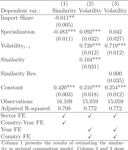
volatility across countries can be explained by the increasing trade openness across countries
observed during recent decades. Using the World Input-Output database, we provide
evidence that the main mechanism through which trade openness negatively affect volatility
is that sectors that rely on imports for their production process are likely to depend more on
global shocks to the industry and less to domestic cycles (Kraay and Ventura, 2007).1 Thus,
trade facilitates higher dissimilarity among the sectors of an economy, diminishing overall
volatility. Finally, we document that changes in the idiosyncratic volatility component are
not only explained by trade openness but also by the volatility in the monetary policy
across countries, acting as an effective business cycle stabilization tool, at the global level.
Although, policy makers are currently more constrained than in the past to stabilize output
fluctuations due to the substantial decline in the importance of the idiosyncratic volatility
component.
Our paper is related to two strands of the literature. First, the literature focused on
evaluating common patterns in macroeconomic volatility, and its shock propagation, from
a global perspective. Commonalities in output volatility have been studied by Stock and
Watson (2005) and Del Negro and Otrok (2008) for the G7 economies, and by Mumtaz and
Theodoridis (2017), Everaert and Iseringhausen (2018) and Carriero et al. (2018a) for 11,
16 and 19 advanced economies, respectively. Up to our knowledge, this is the first study in
providing a global assessment of commonalities in macroeconomic volatility, by addressing
the volatility shock propagation between a large set of advanced and emerging economies.2
Our work is also related to the growing literature on economic uncertainty. There are
numerous proxies for economic uncertainty, based on news (Baker et al. (2016)), the
dis-persion of earnings forecast, the disdis-persion of productivity shocks, the disdis-persion between
forecasters for economic variables, stock market volatility or GDP volatility, among
oth-ers.3 Carriero et al. (2018b) focus on measuring uncertainty and its effect on the U.S.
economy by using a large VAR model with errors whose stochastic volatility is driven by
two common and interrelated unobservable factors, representing aggregate macroeconomic
and financial uncertainty. Recently, Carriero et al. (2018a) employ such framework to
( )
4Giovanni and Levchenko (2012) show that the effect of trade shocks to large firms on aggregate volatility
explain two empirical stylised facts: smaller countries are more volatile and more open countries are more volatile.
5Andr´es et al. (2008) analyze how alternative models of the business cycle can replicate this empirical
finding.
uate commonalities in macroeconomic uncertainty for advanced economies, finding that
uncertainty shocks lower output, stock prices, and in some economies lead to an easing of
monetary policy.
Second, the literature focused on evaluating the effect of specific economic factors on
output volatility. Trade and Terms of trade shocks have been documented as important
sources of output volatility in previous studies. Giovanni and Levchenko (2009) find a
positive and economically significant relationship between trade openness and aggregate
volatility.4 Using a small open economy real business cycle model, Mendoza (1995)
esti-mates that roughly one-half of the variation in aggregate output in a sample of the G7 and
23 developing economies can be attributed to terms of trade shocks. Kose (2002) applies a
similar framework and finds that terms of trade shocks can explain almost all of the
vari-ance in output in small open developing economies. Another important factor considered
in previous studies is financial openness. Buch et al. (2005) found that financial openness
increases business cycle volatility in the decades before the 1990s but it has a cushioned
effect in the 1990s. There is also a large literature pointing to the importance ofgovernment
expenditure on output volatility. Buch et al. (2005) and Fat´as and Mihov (2001), among
others, found that large governments are associated with less volatile economies.5 Fat´as
and Mihov (2003) provide empirical evidence that governments that intensively rely on
discretionary spending induce significant macroeconomic volatility which lowers economic
growth.6 Monetary policy shocks also affect output volatility and its effect depend on
the degree of financial integration of the economy (Buch et al. (2005), Sutherland (1996),
Obstfeld and Rogoff (1976)).
Despite the large literature dedicated to study the underlying drivers of output volatility,
previous studies have typically focused on analyzing a particular driving factor of volatility
without accounting for the implications of other potential factors. The only exception is
Malik and Temple (2009), who use a Bayesian Model Averaging approach to study the
structural drivers of output volatility. However, the authors focus only on developing
countries, and more importantly, they focus on explaining only the level (averaged over
time) of output volatility and not its dynamics. To the best of our knowledge, we are the
6The authors emphasize the importance of political factors in the fiscal policy conduct: institutional
first to identify the main macroeconomic factors that explain changes over time in output
volatility accounting for model uncertainty and reverse causality.
The paper is organized as follows. Section 2 proposes the empirical framework to
measure and decompose global volatility fluctuations. Section 3 describes the dynamics
and assess the propagation of macroeconomic volatility. Section 4 investigates the main
underlying economic factors that could explain changes in volatility worldwide. Section 5
concludes.
2
Measuring Commonalities in Volatility
In this section, we propose a framework that is suitable to jointly estimate output
volatil-ity across countries, decompose it into global, regional and idiosyncratic components, and
assess how volatility shocks propagate at the international level. Specifically, the proposed
empirical framework relies on a hierarchical factor structure, that is designed to
simultane-ously (i) estimate and summarize the output volatilities of a large set of economies into a
small number of factors, both global and regional, (ii) identify changes in the contribution
of the global, regional and idiosyncratic components to the output volatility of countries
over time, and (iii) provide a detailed assessment of the transmission of output volatility
shocks at different levels of disaggregation. In sum, we introduce a framework that is well
suited to analyze the VOLatility Transmission Across Grouped Economies, henceforth, it
will be referred to as the VOLTAGE model.
Within this context, it is important to distinguish between comovements in mean and
in volatility, and their corresponding implications. Recently, Ductor and Leiva-Leon (2016)
have documented that after the early 2000s, economies tend to fall in recessions, and rise in
expansions, in a synchronous way more often than before that time. Hence, if this pattern
persists during future episodes of global recessions, the number of countries affected by
contractionary shocks will be similar or even larger than during the “Great Recession”.
These assessments are based on synchronization of business cycle phases, which rely on
first order moments of output growth. However, it still remains uncertain whether the
severity of GDP downturns is more or less likely to be similar across countries during
next global recessions. If an adverse scenario for the global economy is when most of the
countries enter recessionary phases, an even more drastic scenario is when, in addition, the
is crucial to assess commonalities in the width of international output growth fluctuations,
that is, second order moments, by also accounting for commonalities in first order moments.
Our modelling strategy closely follows the work of Kose et al. (2003), who rely on a
factor structure to decompose real activity growth across countries into global, regional and
idiosyncratic components. However, the authors focus solely on measuring commonalities in
the mean, leaving unaddressed potential volatility comovements. Therefore, we extend their
analysis by also disentangling commonalities in the time-varying macroeconomic volatility
profiles across countries. Consequently, our focus is on “comovement of the volatility”, and
not on “volatility of the comovement”. In particular, previous studies, following the line
of Del Negro and Otrok (2008), have focused on modelling the time-varying volatility of
common mean factors extracted from the data. However, such a modelling strategy is not
designed to measure the extent to which volatility profiles across countries are alike over
time, which is one of the goals of this paper. Instead, the VOLTAGE model is specifically
intended to address commonalities of time-varying volatility measures.
The data employed to estimate the proposed model consists of quarterly real GDP
growth of different countries. This growth rate was computed based on the quarterly
GDP at standardized constant prices in US 2010 dollars. The data was gathered from
Datastream, which has the largest coverage of countries and periods. Since information at
a higher frequency allow us to characterize volatility patterns with more precision, we rely
on data at the quarterly rather than at the annual frequency. Based on data availability,
our sample covers N = 42 countries from four regions of the world, North America, South
America, Europe, and a joint region composed by countries located in Asia and in Oceania.
The list of countries along with the corresponding regions is reported in Table 1. The sample
period spans from 1981:Q1 until 2016:Q3.
Let yik,t be the annual growth rate of quarterly real GDP of country i, which belongs
to region k, at time t. We assume that it is driven by a mean global factor, ¯gt, a mean
regional factor, ¯hk,t, and an idiosyncratic component uik,t, as follows,
yik,t = ¯γik¯gt+ ¯λik¯hk,t+uik,t, (1)
where ¯γik and ¯λik are the corresponding factor loadings, forik = 1,2, ..., nkandk = 1, ..., K,
nk is the number of countries that belong to region k, and K is the total number of
considered regions. Notice that the terms uik,t represent country-specific output growth
uik,t =e
1 2Fik,tεi
k,t, (2)
7Prior to the application of the principal component analysis, the data on output growth is standardized.
Also, to deal with missing data in the extraction of the common factors in the mean, we apply probabilistic principal component analysis.
8However, as a robustness exercises of the empirical analysis, we also extract the mean factors with
filtering techniques by assuming autoregressive dynamics, showing that, besides increasing parameter un-certainty, our main results remain unchanged.
where εik,t ∼N(0,1), Fik,t is a latent variable, and σik,t =e
1
2Fik,t denotes the time-varying
standard deviation associated to country ik. Typically, Fik,t is assumed to be an
inde-pendent univariate autoregressive processes. This functional form was initially used as an
approximation to the stochastic volatility diffusion by Chesney and Scott (1989) and Hull
and White (1987).9 However, given our multi-country environment, we are interested in
de-composingFik,t into its common, regional and idiosyncratic components across countries.10
That is, we decompose country ik log-volatility as follows,
Fik,t = γikgt+λikhk,t+χik,t, (3)
for ik= 1,2, ..., nk and k = 1, ..., K. The term,gt denotes the global volatility factor, while
hk,t denotes the volatility factor associated to the group of countries that belong to region
k, and χik,t denotes the idiosyncratic, or country-specific, volatility component of country
i that belongs to region k.
The global factor measures common changes in the overall degree of countries
macroeco-nomic volatility around the world. Instead, the regional factors account for the
commonal-ities in the volatility patterns between countries located in a given region, after accounting
for global volatility commonalities. Finally, the idiosyncratic component identifies volatility
changes that can be purely attributed to country-specific developments. The coefficients
γik and λik are the corresponding factor loadings and measure the strength of the
comove-9Recent examples of such a modelling strategy are Del Negro and Otrok (2008) and Everaert and
Iseringhausen (2018).
10Such a decomposition is closer to the work by Carriero et al. (2018b), who focuses on measuring U.S.
macroeconomic and financial uncertainty by relying on VAR models.
the dynamics of the mean factors as possible since our main focus is on the comovement in
the volatility. Therefore, we extract mean factors non-parametrically by relying on principal
components.7 This would preclude our main estimates of being significantly affected by
any misspecification in modelling the mean factors.8
Accordingly, in order to investigate volatility commonalities over and above mean
ment between the country-specific volatility and the volatility factors, both at the global
and regional level, respectively.
Equation (3) provides a decomposition of fluctuations in macroeconomic volatility from
a contemporaneous perspective, but it remains silent about potential non-contemporaneous
feedback effects of volatility shocks. Hence, to evaluate the importance of the global
volatil-ity factor on countries macroeconomic volatilvolatil-ity from a more comprehensive perspective,
the latent variables driving both the global and regional volatility factors are assumed to
11We also considered the case when log-volatility factors depend not only on their past values, but also
on past values of the mean factor as a robustness exercise. The results are shown in the empirical Section 3.2.1.
where the innovations are assumed to be normally distributed,ξik,t ∼N(0, σi2k), and
cross-sectionally uncorrelated.
To achieve identification of the factors and factor loadings, we follow Bai and Wang
(2015) and impose two types of restrictions: first, the covariance matrix of the innovations
in the VAR equals to an identity matrix, Σ =IK+1, and second, specific factor loadings,γ11
and {λ1k}Kk=1, are assumed to be lower-triangular matrices with strictly positive diagonal
terms.12 The first restriction facilitates the type of structural analysis that can be performed
with the model since the innovations, ζt, are orthogonal by construction13
12The identification scheme proposed in Bai and Wang (2015) has been proven to work in a context
of linear factor models. Despite the fact that the proposed volatility factor model is nonlinear, those identification restrictions still uniquely identify the factors and factor loadings because the model can be alternatively expressed in a log-linearized representation, which is used to generate inferences from the latent variables (Kim et al. (1998)), as it is shown in Appendix A.1.
13However, notice that since the innovations ζt are orthogonal by assumption, they can be directly
interpreted as structural innovations in an “artificial” way. Therefore, it is important to acknowledge this feature in the interpretations derived from any shock decomposition associated to the VAR defined in Equation (4). Also, notice that if one is interested in allowing Σ to be unrestricted in order to impose a given identification scheme for the structural shocks, it can be also done by imposing stronger restrictions in the matrix of factor loadings, as it is shown in Bai and Wang (2015).
evolve according to a stationary vector autorregresion (VAR),
⎡ ⎢ ⎢ ⎢ ⎢ ⎢ ⎢ ⎣
gt
h1,t .. .
hK,t
⎤ ⎥ ⎥ ⎥ ⎥ ⎥ ⎥ ⎦
= Φ
⎡ ⎢ ⎢ ⎢ ⎢ ⎢ ⎢ ⎣
gt−1
h1,t−1
.. .
hK,t−1
⎤ ⎥ ⎥ ⎥ ⎥ ⎥ ⎥ ⎦
+ζt, (4)
where the innovations are assumed to be normally distributed,ζt∼N(0,Σ). This
assump-tion allows us to perform any type of structural analysis typically employed in a linear VAR
context, but in a perspective of second order moments.11 The dynamics of the idiosyncratic
volatility components are given by independent stationary autoregressive processes,
The proposed VOLTAGE model is suited for a wide range of applications, since it allows
to perform all the types of analyses typically done in the literature of dynamic factor models
and structural vector autoregressions, but for the volatility of data instead of the raw data
itself. Therefore, it can be used to provide a comprehensive assessment on the propagation
pattern of volatility shocks in large dimensional settings.
The model is estimated with Bayesian methods. In particular, we rely on the Gibbs
sampler to provide robust inference on all the elements of the model, that is, latent variables
and parameters. Moreover, the proposed estimation algorithm allows us to deal with
missing observations, which is a typical problem in multi-country GDP data at the quarterly
frequency. The Appendix A.1 reports the details about the estimation procedure.
3
Global, Regional and Idiosyncratic Volatility
The purpose of this section is threefold. First, inferring changes over time in
macroeco-nomic volatility across both developed and developing economies. Second, understanding
the sources of those changes by disentangling them into domestic and foreign
contribu-tions. Third, assessing how macroeconomic volatility shocks propagate throughout the
global economy.
Prior to investigating commonalities in second order moments, it is important to account
for commonalities in first order moments. We extract the common factors in the mean
from the GDP growth of the 42 countries in our sample, as described in Equation 1.
The estimates show that the global factor resembles fairly well the dynamics of the world
real activity, while the regional factors are consistent with several salient features of the
business cycles in those regions, such as, the prolonged slow down in Europe since the late
2000s, the severe recession in Asia due to the 1997 Financial Crisis, the recent downturn
of economic conditions in South America, and the reduction of real activity fluctuations
in North America. Since the focus of this paper is on commonalities in volatility, for the
sake of space, we report the mean factor estimates in A1. Kose et al. (2003), Kose et al.
(2012), and Ductor and Leiva-Leon (2016) provide a deeper assessment on changes in the
comovement of mean output growth at the international level, which is aligned with our
3.1
Cross-country Heterogeneity
We extract commonalities in the volatility profiles of country-specific GDP fluctuations
after removing the common patterns in the mean. The VOLTAGE model is employed to
estimate the volatility, σ2ik,t, of the 42 countries in our sample, and the corresponding
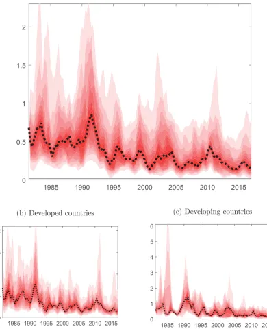
cross-sectional distribution over time is plotted in Figure 1. Chart A plots the world time-varying
second moments distribution, showing two salient features. First, the median of the
cross-sectional distribution exhibits a downward trend, pointing to a moderation of business
cycle fluctuations across the main world economies. Second, the cross-sectional dispersion
of volatility profiles has decreased over time, indicating an increase in the comovement of
international macroeconomic volatility over time. Moreover, in order to assess whether
these two features are consistent with only highly industrialized countries, we compute the
same cross-sectional distribution, but differentiating between developed and developing
economies, plotted in charts B and C, of Figure 1, respectively. The charts indicate these
two features of macroeconomic volatility, downward trend and higher comovement, are
present in both developed and developing countries.
To address whether such an increasing comovement in volatility across countries,
ob-tained with the VOLTAGE model, is an artefact of relying on a factor structure in modelling
second moments, we perform a robustness exercise. We assume no factor structure, and
estimate the time-varying volatility associated to each country, independently, by fitting
univariate stochastic volatility processes to each term uik,t. The results reported in
Fig-ure A2, show the same featFig-ures obtained with the framework based on factor structFig-ure,
indicating an inherent pattern of real activity at the international level. Overall, these
results show that countries macroeconomic volatility has persistently reduced over time
and become more similar worldwide.
In a recent work, Adrian et al. (2019) show substantial changes over time in the
pre-dictive distribution of U.S. GDP growth by relying on quantile regressions.14 Also, Adrian
et al. (2018) document similar patterns at the international level by using quantile panel
regressions. Regarding GDP second moments across countries, Figure 1 suggests that the
14In particular, they show that lower quantiles of GDP growth tend to vary with financial conditions,
especially, when they are deteriorating, while upper quantiles tend to be stable over time.
world macroeconomic volatility distribution is remarkably right-skewed and exhibited
densities associated to all the realizations of volatility, both across time and countries,
within each decade in our sample, that is, 1980s, 1990s, 2000s and 2010s. Chart A of
Fig-ure 2 shows that the world volatility distribution is becoming more right-skewed with time.
This pattern occurs independently on whether we focus only on developed or developing
countries, as shown in Charts B and C.15 This left-displacement of the distribution can be
interpreted as a reduction in the world macroeconomic risk. That is, the realizations of
large and atypical macroeconomic fluctuations across countries has become less frequent
during recent times.
3.2
Dissecting Volatility
The main advantage of the VOLTAGE framework is its ability to endogenously
decom-pose time-varying volatility estimates into the contributions associated to global, regional
and country-specific, or idiosyncratic, development. The time-varying standard deviation
associated to country ik can be compactly expressed as,
σik,t =σg,tγikσhk,tλikσχik,t, (6)
where σg,t = e
1
2gt, σhk,t = e12hk,t, and σχik,t = e12χik,t denote the corresponding global, regional and idiosyncratic components, respectively. Next, we proceed to examine in detail
each of these components and their implications.
3.2.1 Global Component
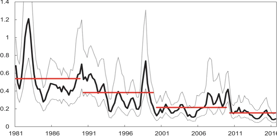
Chart A of Figure 3 plots the dynamics of the global volatility component, showing a
markedly decreasing trend over time. In particular, during the 1980s the average global
volatility was 0.50 standardized units, in the 1990s the average volatility declined to 0.35,
similarly, during the 2000s it continued decreasing reaching 0.20, to finally remain at 0.14
15As a robustness exercise, we also compute the corresponding kernel densities of the time-varying
volatilities obtained with univariate stochastic volatility models. The results, shown in Figure A3, point to the same conclusions.
standard units during the 2010s. Such a persistent decline, which illustrates our first
main result, implies that GDP growth across the main world economies share a feature in
common that can be interpreted as a global moderation of international output fluctuations.
This feature is consistent with the downward trend in the cross-sectional distribution of
16We provide additional evidence on the declining pattern of global macroeconomic volatility based
on three robustness exercises. First, to avoid potential misspecifications in the extraction of the mean common factors, we fit the VOLTAGE model directly to output growth fluctuations, yik,t. Figure A4 plots the estimated global volatility, also showing a persistent declining, with a significant increase during the Great Recession. Second, we estimate the mean and volatility common factors jointly, with Bayesian methods, assuming similar autoregressive dynamics for both types of factors. Figure A5 indicates that, despite increasing the uncertainty around the estimates, the declining pattern in global volatility is also present. Third, to account for the dependence of between the volatility and the mean we allow the volatility factors to depend on their past values and on the lagged mean factors, that is,Ht= ΦHt−1+ Λ ¯Xt−1+ζt, where the log-volatility factors are given by Ht = (gt, h1,t, ..., hK,t) and the mean factors are collected in ¯Xt= (¯gt,¯h1,t, ...,¯hK,t). Figure A6 also shows a persistent decline of the global volatility. These three exercises provide robust evidence on the importance of the global component in the downward trend pattern of macro volatility across countries.
17The weights are obtained by iterating the equations, wj = Bt,jKj, and Bt,j
−1 = Bt,jF −wjG, with Bt|t−1 = I, for j = t−1, t−2, ...,1, where Kj denotes the Kalman gain, and F and G are the matrices corresponding to the transition and measurement equations of the state space representation, respectively, as defined in Appendix A.1. Also, notice that Koopman and Harvey (2003) provide algorithms for computing the weights implicitly assigned to the observed data when estimating the latent variables in a linear state space model. Although the VOLTAGE model works under nonlinear dynamics, it can be expressed in a linearized form by following Kim et al. (1998).
determining international volatility fluctuations. This phenomenon is analyzed in details
in section 3.2.2.16
Next, we examine up to which extent the decline in the global volatility component
has been induced by both, developed and developing economies. For this purpose, we
proceed to disentangle the contribution of each region to the changes exhibited by the
global volatility component. This analysis also allows to identify the regions associated
with the temporary increase in global volatility depicted in Figure 1.
We follow the line of Koopman and Harvey (2003) to decompose the latent factors into
the contributions associated to each of the observable countries real activity. In
partic-ular, we express the state vector containing the latent log-volatilities, both factors and
idiosyncratic,at, as a weighted average of the observed data,
at=
t−1
j=1
wju∗ik,t, (7)
where u∗ik,t = ln(u2
ik,t), and the weights, denoted by wj, can be computed by backward
recursion.17 To facilitate the interpretation of the decomposition, we group all the
country-specific contributions associated to a particular region.
Chart B of Figure 3 shows the historical data decomposition of the global volatility
factor. Notice that the persistent decline in global volatility is not associated to a specific
region, since all the four regions have, in general, significantly contributed to the downward
trend, suggesting that the moderation of macroeconomic fluctuations can be considered as
Regarding global volatility fluctuations, it shows a temporary increase in the early 1980s,
which is accompanied by a significant contribution of the South American region. This is
associated by the period called as the “Lost Decade”. Another increase in global volatility
is observed in the early 1990s. During this period, most of the Western world suffered a
recession. Also, around the same time the German reunification was taking place. This
event had significant economic implications for several European countries. The sudden
increase in global volatility observed in the late 1990s can be rationalized as the result
of spillover effects of the severe Asian crisis to advanced economies through the global
markets. Finally, there is another increase in global volatility that took place between 2007
and 2010, when all the regions contributed almost equally, and that can be associated to
the high levels of uncertainty caused by the adverse effects of the Great Recession.
3.2.2 Regional Components
The regional volatility factors are intended to capture commonalities in output volatility
across countries after accounting for global patterns. We restrict to a definition of groups
based on geographic location of countries since it facilitates the interpretation of the regional
factors, and therefore, the subsequent structural analysis. Figure 4 shows the regional
volatility components along with their corresponding historical data decompositions. Chart
A plots the volatility factor of the North American region, which exhibits three significant
increases. In 1984, all the economies of the region experienced a significant boom leading to
substantial magnitudes of real activity fluctuations. Instead, in 1991, the opposite scenario
occurred, when U.S. and Canada enter a recessionary phase. The third increase can be
attributed to the so called “Tequila Crisis” originated in Mexico. Despite those specific
periods, the volatility in North America has remained relatively stable over time, which
is consistent with Gadea et al. (2018), who showed that since the Great Moderation, U.S.
output growth has remained subdued despite the loss of the Great Recession. Also, the
corresponding decomposition shows that North American volatility is almost no influence
by the volatility of other regions.
Chart B of Figure 4 plots the volatility of South America. This region presents several
temporal increases in volatility, two of them are of a large magnitude. First, the rise in
volatility around the early 1990s is associated to economic upswings in the region due to
policies focused on the liberalization and privatization to incentivize a free market economy.
in the output of Venezuela induced by oil price shocks, and second, uncertainty in the
Argentine economy due to unexpected regulations of its financial system to avoid bank runs.
Similarly to the case of global volatility, temporary increases in regional volatility are not
only related to recessions, but also to large upward fluctuations and to foreign shocks. The
decomposition reveals that North American developments has had a substantial influence
in the volatility of South America during those periods.
Chart C of Figure 4 plots the volatility of the European region. The most significant
episodes of high volatility occurred, first, during the early 1990s European recession, as
dated by the Euro Area Business Cycle Dating Committee. Second, during the Sovereign
Debt Crisis in the early 2010s, event that led to a pronounced declines in real activity for
several countries of the region. Again, the influence of North American developments have
played a substantial role in the volatility of Europe. Finally, Chart D of Figure 4 plots
the volatility associated to the region of Asia+Oceania. The figure shows more frequent
changes in the level of aggregate volatility than for the other regions, such as the one
occurred in the early 2000s, period in which the Turkish economy went through a severe
crisis leading to financial and political instability and to further panic in the markets. In
contrast to South America and Europe, the volatility in Asia+Oceania is mainly driven by
its own developments, being almost no influence by North America.
It is important to notice that all these temporary increases in both global and regional
volatility are not necessarily related to economic recessions. Instead, they seem to be more
generally related to episodes of instabilities, structural changes, and high uncertainty.
3.2.3 Idiosyncratic Components
The idiosyncratic volatility component captures changes in output volatility that can
be attributed to events occurred in a given country and that are unrelated to global or
regional developments, such as domestic economic policies. The estimated idiosyncratic
volatilities, which are plotted in Figures A7 to A9 of the Appendix for the sake of space,
show substantial heterogeneity across countries. For some economies, the idiosyncratic
volatility has remained relatively stable over time, these are the cases of Canada, Mexico,
Belgium or Japan. Instead, other economies exhibit several changes in the idiosyncratic
component of output volatility, for example, Peru, Germany, Norway or China. Also, some
increase due to the 2015 tax inversion practices, in the former case, and to the early 1990s
country-specific depression, in the later.
3.3
Sources of Fluctuations
The effectiveness of stabilization policies would depend on the extent to which
macroe-conomic volatility of a given country is mainly driven by domestic or foreign developments.
Since both global and regional macroeconomic volatility have evolved substantially over
time, it is important to assess the degree of exposition that each country has to
fluctua-tions in these common factors. Therefore, we compute the contribution of global, regional
and idiosyncratic components to the output volatility of each country. The standard
devi-ation of country ik, σik,t can be can be expressed as,
σik,t =Siglobalk,t +S
region
ik,t +S
country
ik,t , (8)
where Siglobalk,t , Siregionk,t , and Sicountryk,t correspond to the share of the global, regional and
idiosyncratic components to the total volatility, respectively, for each period of time. The
expression for each share is derived in the Appendix A.2.18
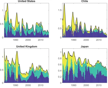
The historical volatility decomposition of four selected countries, United States, United
Kingdom, Chile and Japan, is plotted in Figure 5.19 The figure shows that, in all the four
cases, the volatility has exhibited a downward trend, the contribution of the idiosyncratic
component has lost strength over time, while the contribution of the global component has
increased in recent decades. These results would imply that policy makers of these countries
are currently more constrained to stabilize output fluctuations, by using appropriate tools,
than during the 1980s or 1990s. The historical volatility decomposition for all the countries
in our sample is plotted in figures A10 to A12 of the Appendix, due to space constraints.
The figures show a comprehensive description of the total time-varying output volatility
for each country, along with its corresponding contributions of the global, regional and
idiosyncratic components. This information represents a valuable asset for policy makers,
who are interested in performing timely assessments about the size and sources of
fluctu-18The shares are defined as, Sglobal
ik,t = σik,t
2×logγik gt(σik,t)
αt , S
region
ik,t = σik,t
2×λik hk,tlog(σik,t)
αt , and S country ik,t =
σik,t
2×logχik,t(σik,t)
αt , whereαt=
γikgt
2×log(σik,t) +
λikhk,t
2×log(σik,t) +
χik,t
2×log(σik,t) .
19These countries were selected due to their large size, in economic terms, and because they belong to
ations in macroeconomic volatility for a given country, that is, to disentangle the part of
macroeconomic volatility that is due to purely idiosyncratic (domestic) factors from the
part that can be attributed to regional or global (foreign) developments.
To illustrate the overall patterns, we summarize all the information in figures A10
to A12, from quarters to decades, and from countries to regions. Accordingly, the first
four bars (from left to right) in Chart A of Figure 6 plot the contribution of the global
component, averaged across all the countries in our sample, for the 1980s, 1990s, 2000s and
2010s, respectively. A striking finding is the increase over time in the average contribution
of the global component to the volatility across countries, despite the decrease in global
volatility documented in section 3.1. This feature constitutes our second main result, which
consists of a persistently increasing sensitivity of macro volatility to global developments.
To investigate if this is a particular characteristic of a subset of countries or if it is worldwide
feature, we repeat the same exercise by, separately, using averages across countries that
belong only to each of the four predetermined regions, that is, North America, South
America, Europe and Asia+Oceania. The results presented in the subsequent piles of bars
plotted in Chart A of Figure 6 show that the increase in the contribution of the global
component over time occurred in the four regions under consideration, implying that this
is a systemic feature of international business cycle fluctuations.
Given that the contributions of the three components of volatility are expressed in
terms of shares, and that the global component has increased over time, we assess whether
such an increase has been compensated by a decline in the contribution of the regional
component, or in the idiosyncratic component, or in both. Chart B of Figure 6 plots the
average contribution of the regional component, both across countries in a region and over
quarters in a decade. The figure shows that the sensitivity of output volatility to regional
developments, in general, has remained relatively stable over time, with the exception of
the Asia+Oceania region, which has experienced an increasing sensitivity. Instead, the
average contribution of the idiosyncratic component has persistently declined over time for
all the regions, as can be seen in Chart C of Figure 6.
The overall pattern of the contributions in Figure 6 show that, on average, regional
commonalities account for 37 percent of output volatility fluctuations between 1981 and
2016. Global commonalities accounted for 26 percent of volatility dynamics in the 1980s,
but during the 2010s it accounts for 42 percent. That is, despite the substantial decline
countries has significantly increased. Instead, the contribution of idiosyncratic
develop-ments has dropped substantially from 41 percent in the 1980s, to 18 percent in the 2010s.
This pattern has been roughly similar for North America, South America and Europe.
However, regional commonalities in Asia+Oceania have increased, while the idiosyncratic
component has been significantly loosing importance, pointing to a higher integration in
macro volatility both at the regional and global level for this specific set of countries.
3.4
Shocks Propagation
Economic factors, such as international trade, capital flows, financial integration,
com-mon sectoral composition, have contributed to take the main world economies to a high
level of interconnectedness (Ductor and Leiva-Leon, 2016). The previous sections of this
paper have documented an additional layer of economies interconnection, which is based
on the importance of a global component in determining changes in countries
macroeco-nomic volatility. Global factors, based on strong common patterns, are usually interpreted
as a summary of external influences that countries cannot manage or control, but that at
the same time play an important role in determining country-specific developments (Rey
(2013)). This section provides an assessment on how unexpected increases in the global
component can propagate through countries macroeconomic volatility. This information
could also help policy makers, especially from international organizations, to provide
accu-rate assessment of risks when inferring the outlook of the global economy.
Since the VOLTAGE model allows for endogenous interdependencies between the
com-mon factors of volatility, collected in Ht = (gt, h1,t, ..., hK,t), we are able to apply all the
standard practices used in VAR and FAVAR models to perform structural analysis. In
particular, we rely on the notion of generalized impulse response functions and use the
difference between E(σik,t+j|ζt = 1, ψt−1) and E(σik,t+j|ζt = 0, ψt−1) as our measure of
impulse response, where ψt−1 denotes all the accumulated information up to time t−1.20
Accordingly, to obtain the responses of country-specific volatilities to a one-time unexpected
increases in the volatility factors, we project the impulse response function associated to
the VAR equation by using the corresponding factor loadings,
20Notice that it is not necessary to follow the generalized impulse response function approach of Koop
j
21To identify the latent factors from the factor loadings we follow the line of Bai and Wang (2015) and
assume that Σ =IK+1. An advantage of this identification scheme is that it provides shocks,ζt, that are orthogonal by construction. This feature is also applied in Bai and Wang (2015) to assess spillovers in international bond yields by employing a dynamic factor model in first moments.
∂σik,t+j
∂ζt =exp
1 2
γikΘj[g]+λikΘj[hk]
−1, (9)
for countriesik= 1,2, ..., nk, located in regionsk= 1, ..., K, for horizon path j = 1,2, ..., J,
where Θj[z] denotes the row of Θj that corresponds to the latent factor z ={g, h1, ..., hK},
and where Θj =
∂Ht+j
∂ζt .
21
The responses of country-specific volatilities to a global shock are reported in Figure
(7), showing substantial heterogeneity. In particular, all the three countries composing the
Noth American region are highly sensitive to global shocks. For countries in South America,
Chile is the most responsive to unexpected global developments, while the other countries
of the region present a lower and relatively similar responsiveness. In the case of Europe,
most of the countries experience a significant sensitivity to global shocks, with the exception
of Iceland and Norway. Also, most of the countries that belong to the Asia+Oceania region
are highly sensitive to global volatility shocks, in particular, Indonesia and China. This
impulse response pattern illustrates the high importance of global shocks in influencing
country-specific macroeconomic volatility.
Lastly, we adopt a more aggregate and dynamic perspective in the assessment of shock
propagation and analyze how the influence of global shocks on regional developments has
evolved over time. Once the impulse responses Θj have been estimated, it is possible
to quantify how much a given structural shock explains the historically dynamics of the
log-volatility factors, collected in Ht, by approximating them as follows,
Ht ≈
t−1
j=0
Θjζt−j, (10)
and then computing the corresponding decomposition. Figure 8 plots the shock
decompo-sition of both global and regional log-volatility factors showing a striking feature, which
consists of an increasing contribution over time of global shocks to the volatility dynamics
of all the regions, and more importantly, to the volatility dynamics of the global factor.
This feature corroborates our second main result, which pointed to an increasing
global macro volatility has become “more global”, indicating a more interrelated global
economy in terms of aggregate risks.
4
What Does Explain Changes in Volatility?
In this section, we assess the most robust factors explaining changes in output volatility.
We use Bayesian Model Averaging (hereafter, BMA) to deal with model uncertainty. The
reasoning for doing so is that there are many potential factors that could affect volatility,
however, the theorical literature provides only weak guidance on the specification of the
volatility regression. BMA addresses model uncertainty by weighting the various models
based on fit and then averaging the parameter estimates they produce across models.
4.1
Explanatory Factors
There is ample literature suggesting different potential factors that could explain
vari-ation in volatility. These factors can be categorized as follows:
1) Trade openness. The theoretical relationship between trade openness and output
fluctuations is ambiguous. Trade may affect volatility through three main different channels
(Giovanni and Levchenko, 2009): (i) trade openness may expose industries to external
shocks leading to higher volatility (Newbery and Stiglitz, 1984); (ii) trade may increase
specialization and lead to a less diversified production structure, increasing volatility; (iii)
trade can change co-movement between sectors within the economy; sectors that are more
open to trade will depend more on global shocks to the industry than to domestic cycle,
this may reduce volatility (Kraay and Ventura, 2007).
To compute trade openness we use data on exports and imports and define trade
open-ness in year t as,
Tit =
Eit+Iit
GDPit
(11)
whereEit is the total exports from country iin year t,Iit denotes total imports to country
i in yeart, andGDPit is the nominal GDP in country i in year t.
2) Financial integration. Theoretically, the impact of financial integration on output
volatility is ambiguous. Evans and Hnatkovska (2014) and Kose et al. (2006) emphasize two
main channels through which larger international financial integration may affect output
volatility: (i) consumption paths will be less correlated with country-specific shocks, since
financial instruments facilitates risk-sharing by households; (ii) greater financial
integra-tion increases producintegra-tion specializaintegra-tion within countries, magnifying the effect of
industry-specific shocks and their transmission across countries. The first channel predicts a negative
effect on macroeconomic volatility while the second a positive.
As a measure of financial globalization, we use a financial openness indicator based on
Lane and Milesi-Ferretti (2007). This indicator is defined as the volume of a country’s
assets and liabilities as a share of GDP:22
Fit =
Ait+Lit
GDPit
(12)
where Ait is total assets to GDP and Lit is liquid liabilities to GDP in country i. This
variable has been extensively used in the literature and is considered a good measure in
comparison to available alternatives.
3) Supply shocks. To capture supply shocks we consider exchange rate volatility and
terms of trade volatility. Changes in the exchange rate and terms of trade affect
out-put through two main channels: (i) fluctuations in the exchange rate and term of trades
alter imports and hence affects real domestic income; (ii) inflationary pressures through
fluctuations in domestic spending.
To compute terms of trade we use price level of imports and exports from the Penn
World Table 9.0. Formally, the terms of trade is defined as,
totit= P Eit
P Iit
(13)
where P Eit and P Iit are the price level of exports and imports in country i at year t,
respectively. Since these prices are available per year we compute the volatility at period
t as the square of the first differences in log oftotit fromt−1 to t,
σ(tot)it = (log(totit)−log(totit−1))2 (14)
The square of the growth rate is a standard proxy of volatility in finance (Alizadeh et al.,
2002). We also obtain the exchange rate, defined as national currency units per U.S. dollar,
from the Penn World table 9.0 and compute exchange rate volatility as,
22The original indicator constructed by Lane and Milesi-Ferretti (2007) is based on country’s foreign
σ(xr)it = (log(xrit)−log(xrit−1))2 (15)
5) Monetary policy shocks. The impact of monetary policy shocks on output volatility
has been extensively study. Traditional models suggest that monetary contractions
(ex-pansions) should increase interest rate (decrease), lower (raise) prices and reduce (increase)
real output. Thus, changes in interest rate volatility may also affect output volatility.
Fern´andez-Villaverde et al. (2011) consider a non-linear small open economy DSGE model
to show that as real interest rate volatility increases, countries reduce their foreign debt
by reducing consumption. Thus, investment falls, as foreign debt becomes a less
attrac-tive hedge for productivity shocks, leading to a fall in output. Empirically, Mumtaz and We use both volatilities σ(tot) and σ(xr) to test the importance of supply shocks in
ex-plaining changes in output volatility over time.
4)Fiscal policy shocks. In theory, governments may use discretionary changes to smooth
out fluctuations in output. Some of these discretionary changes include expansionary
spend-ing and tax cuts in recessions and contractionary policy in expansions. However, there is
no agreement as to whether fiscal policy volatility increases or decreases macroeconomic
volatility. Gali (1994) show that both low income tax rate and higher share of government
expenditure are asssociated with low output volatility in a real business cycle model,
how-ever, the predicted effects are small. Fat´as and Mihov (2003) and Fat´as and Mihov (2001)
provide empirical evidence that governments that intensively rely on discretionary
spend-ing induce significant macroeconomic volatility. Fern´andez-Villaverde et al. (2015) find
that unexpected changes in fiscal volatility can have a sizable adverse effect on economic
activity. Andr´es et al. (2008) found a negative effect of government size on business cycle
volatility. Grechyna (2019) shows that higher fraction of discretionary public spending in
total public spending, other things being equal, leads to more volatile business cycles.
To account for the potential effect of fiscal policy on volatility we use the share of
government consumption as in Fatas and Mihov (2013). This variable is obtained from
the Penn World Table 9.0. Since government consumption is only available per year we
compute the volatility at periodt as the squared of growth of government expenditure from
t−1 to t,
σ(gov)it =
govit−govit−1
govit−1
2
23There is ample empirical literature examining the impact of monetary policy shock on output, see
surveys in Christiano et al. (1999) and Bagliano and Favero (1998).
24For a detailed description, see Feenstra et al. (2015).
Zanetti (2013) using a SVAR with stochastic volatility found that the nominal interest rate,
σit =ρσit−1+σ(xk)itβk+μt+αi+vit, (19)
where σit is the quarterly average volatility of economic growth in country i at year t,
as obtained with the framework proposed in Section 2, and shown in figures A10-A12. inflation, and output growth fall after an increase in the volatility of monetary policy.23
We measure monetary policy volatility using the square of the growth rate of the
short-term lending interest rates obtained from the World Bank Development Indicator.
For-mally,
σ(int)it =
intit−intit−1
intit−1
2
(17)
where intit is the short-term interest rate at year t in country i.
6) Technology shocks. The role of technology shocks in business cycle fluctuations has
been widely studied in the real business cycle models that followed the seminal work by
Kydland and Prescott (1982). Overall, there is consensus in the literature that
expan-sions in output, at least in the medium-long run, are caused by TFP increases that derive
from technical progress (Rebelo, 2005). Prescott (1986) estimated that technology shocks
could account for around 75% of business cycle fluctuations. Changes in technology factor
productivity could then be an important factor leading to changes in output volatility.
Total factor productivity (hereafter TFP) level was obtained from the Penn World Table
9.0 (variable ctfp). It is computed using output-side real GDP, capital stock, labor input
and the share of labor income of employees and self-employed workers in GDP.24 We then
measure volatility in TFP as the square growth rate of TFP,
σ(T F P)it =
T F Pit−T F Pit−1
T F Pit−1
2
(18)
where T F Pit is the TFP at year t in country i.
4.2
Model Uncertainty
Following Ductor and Leiva-Leon (2016) we use a BMA panel data approach to deal
with model uncertainty in assessing the most robust explanatory factors of output volatility
25Using a BMA approach, Malik and Temple (2009) find that remote countries exhibit greater output
volatility. However, Malik and Temple (2009) focus on time-invariant drivers of the constant volatility, using only cross-sectional information. Instead, our paper analyses the drivers of changes in volatility, which can be interpreted as its short-run dynamics.
26We also consider a beta-binomial prior for the model space and different forms of the hyperparameter
g in the robustness section.
We acknowledge the potential inefficiency of our estimates due to the measurement error
associated to the dependent variable. Therefore, we perform a series of robustness tests to
assess the reliability of our results. The term σ(xk)it includes a set of potential drivers as
defined in Section 4.1. We include time year dummies in all the regressions, μt, to account
for time aggregate effects, i.e. unobservables affecting all countries, such as oil prices. αi
captures all time invariant factors of the countries, such as geographical location; vit is
the disturbance term.25 The main idea of the BMA approach is to compute a weighted
average of the conditional estimates across all possible models resulting from different
combinations of the regressors. The weights are the probabilities, obtained using Baye’s
rule, that each model is the “true” model given the data. We use the priors specified in
Magnus et al. (2010). In particular, Magnus et al. (2010) considers uniform priors on the
model space, so each model has the same probability of being the true one. Moreover, they
use a Zellner’s g-prior structure for the regression coefficients and sets the hyperparameter
g = max(1N,K2), as in Fernandez et al. (2001), whereK is the number of regressors andN the
number of observations.26 This hyperparameter measures the degree of prior uncertainty
on coefficients.
In the next section, we present the estimates of theposterior inclusion probability (PIP)
of an explanatory factor, which can be interpreted as the probability that a particular
regressor belongs to the true model of international output volatility. We also present
results on the posterior mean, the coefficients averaged over all models, and the posterior
standard deviation, which describes the uncertainty in the parameters and the model.
4.3
Main Drivers of Volatility
We first present results for all the countries in a static panel, without lags of output
volatility as regressors. Table 2 reports the estimates of the output volatility model obtained
by using the BMA panel approach over the 1981-2014 period for 37 emerging and advanced
economies. Column 1 presents the posterior inclusion probability of each potential driver of
output volatility. The rule of thumb is that a factor is considered very robust if the PIP is


![State aids to shipbuilding [1st report] Reports from the Commission to the Council and the European Parliament COM (79) 672 final, 28 November 1979](data:image/gif;base64,R0lGODlhAQABAIAAAP///wAAACH5BAEAAAAALAAAAAABAAEAAAICRAEAOw==)