BLIND DECONVOLUTION USING SHEARLET -TV REGULARIZATION
Z. MOUSAVI1, R. MOKHTARI1, M. LAKESTANI2, §
Abstract. In this article we propose two minimization models for blind deconvolution. In the first model, we use shearlet transform as a regularization term for recovering image. Also total variation method is used as a regularization term for point spread function(PSF). To speed up the process, Fast ADMM approach is exploited. In the second model, shearlet transform is utilized as a regularization term for both image and PSF.
Keywords: shearlet, total variation, blind deconvolution, Fast ADMM, Image processing.
AMS Subject Classification: 94A08, 97N40, 68U10.
1. Introduction
The goal of image deblurring is to estimate an image with the high quality, which has been degraded by camera motion, also the noise resulted from the imaging devices. When the degradations can be modeled as a convolution operation, the act of restoring the original image from the degraded blurred image, frequently called deconvolution [1]. We denote the model of degradated image as
h⊗f +n, (1)
wherehis a convolution kernel or point spread function (PSF) of the imaging system,f is the original image andn is Gaussian white noise . Recoveringf andh using only the degraded image g is called blind deconvolution [2]. Several methods presented the recovering of the deblurred image and PSF in (1) simultaneously. Nakagi et al. [3] presented a VQ-based blind image restoration algorithm. Panchapakesan et al. [4] introduced a blur identification method from vector quantizer encoder distortion. The authors of [5, 6, 7] used inverse filtering methods and Cannon used a Tikhonov regularization[9]. Liao et al. used a GCV approach [13]. We refer to [2, 11-16, 21-25] and references therein, for more informations in blind deconvolution.
Blind image deconvolution is an ill-posed problem [13], hence You and Kaveh designed in [20] a regularizing approach to join blur identification and image restoration. They considered
1 Department of Mathematical Sciences, Isfahan University of Technology, Isfahan 84156-83111, Iran.
e-mail: [email protected]; ORCID: https://orcid.org/0000-0002-2240-4837. e-mail: [email protected]; ORCID: https://orcid.org/0000-0002-1420-0949.
2
Faculty of Mathematical sciences, University of Tabriz, Tabriz, Iran.
e-mail: [email protected]; ORCID: https://orcid.org/0000-0002-2752-0167. § Manuscript received: May 23, 2017; accepted: October 9, 2017.
TWMS Journal of Applied and Engineering Mathematics, Vol.9, No.3 cI¸sık University, Department of Mathematics, 2019; all rights reserved.
the following problem:
minf,hkf⊗h−gk22+λ1kDfk22+λ2kDhk22, (2)
where D is the first-order differencing matrix, λ1 and λ2 are the two positive regulariza-tion parameters which weigh their contriburegulariza-tion. Also Chan and Wong [21] investigated the following blind deconvolution problem:
minf,hkf⊗h−gk22+λ1T V(f) +λ2T V(h). (3)
The definition of discrete TV norm will be given in section IV. Total variation regularization model (3) has superior performance when applied to piecewise constant images but it becomes less effective when images contain complex textures and edges.
The multiscale and multidirectional features of the shearlet transform provide a good estimation ability for restoring images which are more complicated.
According to this point, in this article, we consider two blind deconvolution models. In the first model, shearlet transform is employed as a regularization term for recoveringf (original image) and the total variation regularization is used for restoring h. In the second model shearlet transform is used for concurrent restoringf and h(point spread function) from the observation imageg.
Alternating direction method of multipliers (ADMM) is a common tool for solving min-imization problems. ADMM with a predictor-corrector-type acceleration stage results to accelerated variant of ADMM to solve minimization problem. This method is called Fast ADMM [27]. Here we solve minimization problems using the ADMM and Fast ADMM methods.
The rest of the paper is structured as follows. In Section 2, the shearlet transform and its implementation are described. We solve a deconvolution minimization problem using Fast ADMM method in section 3. In section 4, we present two blind deconvolution models. Experimental results are presented in section 5, and finally we conclude the paper in section 6.
2. Shearlet Transform
The shearlet transform is a directional representation system based on anisotropic dilation which is able to describe geometry of multidimensional functions [28]. Letψ∈L2(R2) and
Aa=
a 0 0 √a
, Bs =
1 s
0 1
,
whereAais an anisotropic dilation matrix andBsis a shear matrix. The Continuous Shearlet System SH(ψ) is defined by
SH(ψ) ={ψa,s,t(x) =a−3/4ψ(A−a1Bs−1(x−t)) :a >0, s∈R, t∈R2}. (4) The continuous shearlet transform of a functionf ∈L2(R2) is given by
f ∈L2(R2)−→SHψ(f)(a, s, t) =< f, ψa,s,t > . (5) However, disadvantage of defined shearlet system is bias toward certain axis. This prob-lem is circumvented by definition cone-adapted discrete shearlet system. Furthermore, all the bandwise discrete shearlet transforms can be computed effectively by employment the discrete Fourier transform and the discrete inverse Fourier transform . LetSHi(f) represents the discrete shearlet transform off that isith subband of the shearlet transform. Moreover, suppose H1 is the fast Fourier transform or FFT of the discrete 2D scaling function, and Hi(i≥2) are those of the discrete shearlets [29].
3. Deconvolution by Fast ADMM method
In this section, we formulate the deconvolution problem as follows:
minf
µ
2kf⊗h−gk
2 2+λ
N X
i=1
kSHi(f)k1, (6)
where SHi(f) is the ith subband of the shearlet transform of f. Introducing auxiliary variables wi,(i= 1, ..., N),(6) is equivalent to
minf,wi µ
2kf⊗h−gk
2 2+λ
N X
i=1
kwik1, (7)
SHi(f) =wi i= 1,2, ..., N. (8)
Introducing the dual variableP ={pi}Ni=1, and applying Fast ADMM for solving (7), we get
the following algorithm:
Algorithm 1: Fast ADMM for deconvolution
Input: convolution operatorh, observed imageg, β1 = 1, P = 0.
for k= 1,2,3, ... do 1. wik= arg minwi kwik1+
α1
2 kwi−SHi(f) +p
k
ik22, i= 1,2, ..., N,
2. f¯k = arg minf¯ µ
2k ¯
f ⊗h−gk2 2+
λα1
2 PN
i=1kSHi( ¯f)−wki −pkik22,
3. p¯ki+1=pk
i +γ(SHi( ¯fk)−wki), i= 1,2, . . . , N,
4. βk+1= (1 + p
1 + 4(βk)2)
2 ,
5. fk+1 = ¯fk+β k−1
βk+1 ( ¯f
k−f¯k−1),
6. pik+1= ¯pki +
βk−1
βk+1 (¯p
k+1
i −p¯ki), i= 1,2, . . . , N, 7. λ=λ∗.98,
end
In step 1, the explicit formulas for wik is:
wi = shrink(SHi(f) +pi,1/α1), i= 1, ..., N,
where shrink(a, b) = sgn(a).∗max(|a| −b,0).
In step 2, to solve the ¯f-subproblem, we have SHi( ¯f) =Hi.∗fft2( ¯f), therefore:
¯
f = ifft2(µ∗conj(fft2(h)).∗fft2(g) +α1λ PN
i=1(Hi.∗fft2(wi−pi))
PN
i=1α1λ(Hi.∗Hi) +µ∗conj(fft2(h)).∗fft2(h)
),
where fft2 is 2-D Fourier transform and ifft2 is inverse 2-D Fourier transform.
Fast alternative direction method is used in process solving proposed model for restoring original image in next section.
4. Proposed Algorithms
In this section, we present two models for blind deconvolution problem. A. Blind deconvolution by SH-TV regularization
In the first form, we apply shearlet transform as a regularization term of an image and use the total variation method as regularization term of PSF. This can be written as:
minf,h
µ
2kf⊗h−gk
2
2+λ1khkT V +λ2
N X
i=1
whereSHi(f) is theith subband of the shearlet transform of f. The TV-norm,khkT V,can either be the anisotropic TV norm :
khkT V = X
i
|(Dxh)i|+|(Dyh)i|, (10)
or the isotropic TV norm :
khkT V = X
i q
(Dxh)2i + (Dyh)2i, (11)
where Dxh = vec(h(x+ 1, y)−h(x, y)), Dyh =vec(h(x, y+ 1)−h(x, y)). Here we apply anisotropic TV norm. The isotropic TV, can be similarly derived.
Without using a priori information, let initial f be the observed image and initial h be the delta function in our numerical results. Iterative procedure for solving the problem (9) is formulated in Algorithm 2 :
Algorithm 2
Input: an initial image f, an initial PSF h and an observed imageg
for k= 1,2,3, ... do 1. Solve for hk :
hk = arg minh
µ
2kf
k−1⊗h−gk2
2+λ1khkT V, (12)
2. Solve for fk :
fk= arg minf
µ
2kf ⊗h
k−gk2 2+λ2
N X
i=1
kSHi(f)k1. (13)
end
a. h-Subproblem: The minimization problem (9) may not have a unique solution. For obtaining an acceptable solution, natural and physical conditions onf andhcan be imposed as what follows [21],
h≥0, X
i,j
hi,j = 1, f ≥0. (14)
Let D = (Dx, Dy), therefore khkT V =kDhk1 and hence the minimization problem (12)
can be rewritten as:
minh
µ
2kf⊗h−gk
2
2+λ1kDhk1, (15)
which is equivalent to:
minh,z
µ
2kf ⊗h−gk
2
2+λ1kzk1, (16)
s.t z=Dh. (17)
Introducing the dual variable y, the augmented Lagrangian can be written as
h= arg minz,hkzk1+ µ
2λ1kf⊗h−gk 2
2+< y, z−Dh >+ηrkDh−zk22. (18)
For the estimating of PSF in (18), letting ˆf =F(f), the convolution operator can be written asf⊗h=F∗ΛF h, where Λ is a diagonal matrix with diagonal entries ˆf. LetM =F∗ΛF, therefore :
h= arg minz,hkzk1+ µ
2λ1
kM h−gk22+< y, z−Dh >+ηrkDh−zk22. (19)
Figure 1. Original images : Cameraman, Peppers, Shepp-Logan, Satellite (from left to right).
for k= 1,2,3, ... do 1. hk+1 = arg minh
µ
2λ1kM h−gk 2
2−< y, z−Dh >+ηrkz−Dhk2, 2. zk+1= arg minzkzk1−< y, z−Dhk+1>+ηrkz−Dhk+1k2, 3. yk+1 =yk−ηr(zk+1−Dhk+1),
4. ηr=
δηr, ifkzk+1−Dhk+1k2 ≥ξkzk−Dhkk2
ηr, otherwise.
end
To solve step 1, by considering normal equations, we have:
(µM∗M+ηrD∗D)h=µM∗g+ηrD∗z−D∗y. (20)
Using the Fourier transform, Eq. (20) will have the following solution:
h=F∗
F(µM∗g+ηrD∗z−D∗y)
µ|F M|2+η
r(|F Dx|2+|F Dy|2)
. (21)
In step 2, the explicit formulas for z is:
z= shrink(Dh+ 1
ηr
y,1/ηr).
b. f-Subproblem: We use Fast alternative direction method for restoring original image ,f, similar to section 3.
B. blind deconvolution by SH-SH regularization
In the second model, shearlet transform is used as regularization term of an image and PSF as:
minf,h
µ
2kf⊗h−gk
2 2+τ1
N X
i=1
kSHi(h)k1+τ2
N X
i=1
kSHi(f)k1. (22)
To solve this problem, we propose the following algorithm : Algorithm 4.
Input: an initial image f, an initial blur h and an observed imageg
1.for k= 1,2,3, ... do 2. Solve for hk:
hk = arg minh
µ
2kf
k−1⊗h−gk2 2+τ1
N X
i=1
kSHi(h)k1, (23)
3. Solve for fk:
fk = arg minf
µ
2kf ⊗h
k−gk2 2+τ2
N X
i=1
kSHi(f)k1, (24)
end
0 2
4 6
8
0 2 4 6 8 0.016 0.018 0.02 0.022 0.024
Observed Image, BSNR:30dB
0 5
10 15
20
0 5 10 15 20
0 0.005 0.01 0.015 0.02 0.025 0.03
0
5
10
0 5 10
0 0.1 0.2 0.3 0.4 0.5
5. Numerical Results
Here, we use the presented methods (Shearlet-Total variation blind deconvolution (SH-TV BD) and Shearlet-Shearlet blind deconvolution (SH-SH BD)) for restoring degraded image and PSF for some images with different kinds of PSFs and noise levels. We use peak signal to noise ratio (PSNR) and improvement in signal-to-noise ratio (ISNR) to measure the quality of the restored images. Also blurred signal-to-noise ratio (BSNR) is used to measure the noise contained in observed image, which are defined as follows:
PSNR = 20log10 255
kf−uk2
, ISNR = 20log10kf−gk2
kf−uk2
, BSNR = 20log10kgk2
knk2 ,
where f, g, u and n, are the original image, observed image, recovered image and the noise vector respectively. In all tests, we use the observed image as an initial image and the delta function as an initial PSF. Table 1 displays the results for Peppers, Cameraman,
Shepp-Table 1. Comparison result in PSNR, blurred image by Gaussian(7,5),
BSNR=30 dB.
blured Sh-TV BD SH-SH BD non-blind [32]
Peppers 24.73 23.36 27.42
Cameraman 24.10 22.11 26.74
Shepp-Logan 29.71 24.79 34.37
Satellite 30.28 27.23 31.02
Logan and Satellite images presented in Figure 1. Images degraded by Gaussian PSFs with variance 5 of size 7 and Gaussian noise with BSNR=30dB. For all images in SH-TV blind deconvolution, parameter λ1 is varying from 106 to 108 and λ2 = 0.2.Table 1 shows
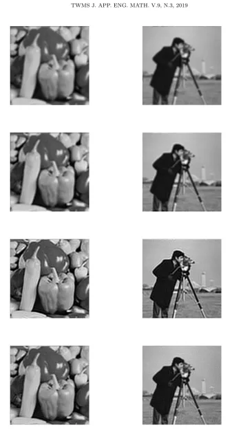
that the results of the presented blind deconvolution methods (specially SH-TV method), is comparable to that of the nonblind deconvolution one. Figure 2 shows the obtained results using shearlets-total variation blind deconvolution, shearlet-shearlet blind deconvolution and Fast ADMM deconvolution where PSF is known, for Peppers and Cameraman images.
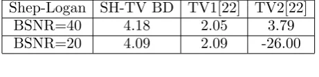
We also compare the Shearlet-Total variation blind deconvolution method with the blind deconvolution algorithms in [21, 22]. Obtained results are in Tables 2 and 3. In [21] authors used total variation function as the image and the point spread function priors. In [22] authors used the total variation function as the image prior and a simultaneous autoregressive (SAR) model as the PSF prior. In these tests, the Cameraman and Shep-Logan images, degraded by Gaussian PSFs with variance 5 of size 10 and Gaussian noises with BSNR=40dB and 20dB. The parameter λ1 is varying from 106 to 108 and λ2 = 0.2. It can be observed
that for the Gaussian PSF, the SH-TV blind deconvolution method outperforms the other three methods. Figure 3, shows the results of presented methods on Satellite image degraded by kernel gaussian(7,5) and BSNR=30.
Table 2. Comparison in ISNR on Gaussian PSF with variance 5.
Cameraman SH-TV BD TV1[22] TV2[22] Method[21]
BSNR=40 1.58 1.66 2.49 1.32
Table 3. Comparison in ISNR on Gaussian PSF with variance 5 .
Shep-Logan SH-TV BD TV1[22] TV2[22]
BSNR=40 4.18 2.05 3.79
BSNR=20 4.09 2.09 -26.00
6. Conclusions
In this paper we presented two blind deconvolution methods: SH-TV method and SH-SH method. By using of shearlet transform, we are able to restoring more details of images with complex tissues. Obtained results show the efficiency of the presented methods for image recovering in minimization problems. Also our results for blind deconvolution, is comparable to those of the nonblind deconvolution.
References
[1] Patel, V. M., Easley, G. R. and Healy, D. M.,(2009) Shearlet-Based Deconvolution, IEEE Trans. Image Process, 18(12) pp. 2673-2685.
[2] Campisi, P. and Egiazarian, K. ,(2007) Blind Image Deconvolution: Theory and Applications. Boca Raton, FL: CRC.
[3] Nakagaki, R. and Katsaggelos, A. K., (2003) , A VQ-based blind image restoration algorithm, IEEE Trans. Image Process., 12(9) pp. 1044-1053.
[4] Panchapakesan, K. Sheppard, D. G. Marcellin, M. W. and Hunt, B.R. (2001), Blur identification from vector quantizer encoder distortion, IEEE Trans. Image Process., 10(3) pp. 465-470.
[5] Kundur, D. and Hatzinakos, D.(1998) , A novel blind deconvolution scheme for image restoration using recursive filtering, IEEE Trans. Signal Process., 46(2) pp. 375-390.
[6] Ng, M. Plemmons, R. and Qiao, S. (2000), Regularization of RIF blind image deconvolution, IEEE Trans. Image Process., 9(6) pp. 1130-1134.
[7] Ong, C. and Chambers, J.(1999), An enhanced NAS-RIF algorithm for blind image deconvolution, IEEE Trans. Image Process., 8(7) pp. 982-992.
[8] Stockham,T. G. Cannon, T. M. and Ingebretsen, R. B., (1975), Blind deconvolution through digital signal processing, Proc. IEEE, 64(4) pp. 678-692.
[9] Cannon, M.,(1976), Blind deconvolution of spatially invariant image blurs with phase,IEEE Trans. Acoust., Speech, Signal Process., 24(1) pp. 58-63.
[10] Lane, R. G. and Bates, R. H. T., (1987) , Automatic multidimensional deconvolution, J. Opt. Soc. Amer. A, 4(1) pp. 180-188.
[11] Katsaggelos, A. and Lay, K., (1989), A. Katsaggelos and K. Lay, Simultaneous blur identification and image restoration using the EM algorithm, in Proc. SPIE Conf, Visual Commun. Image Process. IV, 1199 pp. 1474-1485.
[12] Lagendijk, R. Tekalp, A. and Bidmond, J., (1990) Maximum likelihood image and blur identification: A unifying approach, Opt. Eng., 29 pp. 422-435.
[13] Liao, H. and Ng, M. K., (2011), Blind deconvolution using generalized cross-validation approach to regularization parameter estimation, IEEE, Transactions on Image Processing, 20(3) pp. 670-680. [14] Likas, A. C. and Galatsanos, N. P., (2004), A variational approach for Bayesian blind image
deconvolu-tion, IEEE Trans. Signal Process., 52(8) pp. 2222-2233.
[15] Molina, R. Mateos, J. and Katsaggelos, A. K., (2006), Blind deconvolution using a variational approach to parameter, image, and blur estimation, IEEE Trans. Image Process., 15(12) pp. 3715-3727.
[16] Tzikas, D. Likas, A. and Galatsanos, N., (2009) Variational Bayesian sparse kernel-based blind image deconvolution with student’s-t priors, IEEE Trans. Image Process., 18(4) pp. 753-764.
[17] Reeves, S. and Mersereau, R., (1992) Blur identification by the method of generalized cross-validation, IEEE Trans. Image Process., 1(3) pp. 301-311.
[18] Miskin, J.W. and MacKay, D. J. C., (2000) Ensemble learning for blind image separation and deconvo-lution, in Advances in Independent Component Analysis, M. Girolami, Ed. New York: Springer-Verlag. [19] Adami, K. Z., (2003), Variational methods in Bayesian deconvolution, PHYSTAT2003, SLAC, Stanford,
California, pp. 8-11.
[21] Chan, T. F. and Wong, C. K., (1998) Total variation blind deconvolution, IEEE Trans. Image Process., 7(3) pp. 370-375.
[22] Babacan, S. D. Molina, R. and Katsaggelos, A. K., (2009), Variational Bayesian blind deconvolution using a total variation prior, IEEE Trans. Image Process., 18(1) pp. 12-26.
[23] You, Y. and Kaveh, M., (1999), Blind image restoration by anisotropic regularization, IEEE Trans. Image Process, 8(3) pp. 396-407.
[24] Huang, Y. and Ng, M. (2008), Lipschitz and total-variational regularization for blind deconvolution, Commun. Comput. Phys., 4 pp. 195-206.
[25] Kundur, D. and Hatzinakos, D. , (1996), Blind image deconvolution, IEEE Signal Process. Mag., 13(3) pp. 43-64.
[26] Rudin, L. Osher, S. and Fatemi, E., (1992), Nonlinear total variation based noise removal algorithms, Physica D, 60 pp. 259-268.
[27] Goldstein, T. O’Donoghue, B. Setzer, S. and Baraniuk, R., (2014), Fast Alternating Direction Optimiza-tion Methods, SIAM J. Imaging Sciences, 7(3) pp. 1588-1623.
[28] Kutyniok, G. and D. Labate, D., (2009), Resolution of the wavefront set using continuous shearlets, Trans. Am. Math. Soc., 361 pp. 271-2754.
[29] Guo, W. Qin, J. and Yin, W., (2014), A New Detail-Preserving Regularization Scheme, SIAM J. Imaging Sciences, 7(2) pp. 1309-1334.
[30] Hauser, S., (2012) Fast Finite Shearlet Transform, preprint, arXiv:1202.1773.
[31] Chan, S. H. Khoshabeh, R. Gibson, K. B. Gill,P. E. and Nguyen, T. Q., (2011), An Augmented La-grangian Method for Total Variation Video Restoration,IEEE Trans. Image Process., 20(11) pp. 3097-3111.
[32] He C., Hu, C. and Zhang, W., (2014), Adaptive shearlet-regularized image deblurring via alternating direction method, Multimedia and Expo (ICME), IEEE International Conference.
Zohre Mousavi Rizi was born 1982 in Iran. She received the B.Sc degree
in Applied mathematics in 2004 and the M.Sc degree in Pure Mathematics in 2006, both from the University of Yazd in Iran and currently pursuing the Doctor degree in Applied mathematics at Esfahan Technology university in Iran . Her research interests include: Image processing, shearlet and minimization methods .
Reza Mokhtari received his Ph.D. in Applied Mathematics (Numerical
Anal-ysis) in 2005 at Iran University of Science and Technology in Tehran, Iran. Since 2005 he has been working at the Department of Mathematical Sciences of Isfahan University of Technology, Isfahan, Iran. He is currently an associate professor and his main research interest is numerical solution of differential equations.
Mehrdad Lakestani is a Professor at Department of Applied Mathematics in