Vol. 7, No. 2, 2015 Article ID IJIM-00554, 11 pages Research Article
Numerical solution of the one dimensional non-linear Burgers
equation using the Adomian decomposition method and the
comparison between the modified Local Crank-Nicolson method and
the VIM exact solution
AR. Haghighi∗†, M. Shojaeifard ‡
————————————————————————————————–
Abstract
The Burgers equation is a simplified form of the Navier-Stokes equations that very well represents their non-linear features. In this paper, numerical methods of the Adomian decomposition and the Modified Crank Nicholson, used for solving the one-dimensional Burgers equation, have been com-pared. These numerical methods have also been compared with the analytical method. In contrast to the conventional Crank-Nicolson method, the MLCN method is an explicit and unconditionally stable method. The Adomian decomposition method includes the unknown function U (x), in which each equation is defined and solved by an infinite series of unbounded functions. Velocity parameters u in the direction of the X axis, are examined at different times with different Reynolds numbers over a fixed time step. Also the accuracy of the Adomian and the Crank-Nicolson methods at different Reynolds numbers have been studied using two examples with different initial conditions, and the Adomian decomposition method is closer to the analytical method.
Keywords : Non-linear Burgers equation; Adomian method; the modified Local Crank-Nicolson method.
—————————————————————————————————–
1
Introduction
T
hNavier-Stokes and the continuity equations,e Burgers equation is a special form of the which was introduced in 1915 by Bateman [1]. In this equation continuity and pressure components of the Navier-Stokes is omitted. Burgers equation is a fundamental partial differential equation of the fluid mechanics [2]. This equation is widely used in many physical phenomena, such as mod-els of gas dynamics, plasma dynamics,simula-∗Corresponding author. [email protected] †Department of Mathematics, Urmia University of Technology, Urmia, Iran.
‡Department of Mathematics, Urmia University of Technology, Urmia, Iran.
tion of traffic flows, shock wave, simplified model of the behavior of the boundary layer, sound at-tenuation in fog, etc [3, 4, 5, 6, 7, 8, 9, 10, 11]. Because of their widespread use, these equations have been studied by many researchers and are appropriate context for research activities and several studies about different, accurate and ex-plicit numerical solutions are done to generalize these equations to higher dimensions [12]. Differ-ent numerical methods such as the finite differ-ence, the finite element, and the spectral meth-ods, are used for solving the Burgers equations [13, 14, 15, 16]. In recent years, the Adomian decomposition method (ADM) has been consid-ered by many researchers for solving the Burgers equation [17,18]. Our best strategy, which hasnt
yet been used for solving the Burgers equation is the ADM discretization method. The ADM dis-cretization method was first utilized for obtaining numerical solutions, to discretize the nonlinear Schrdinger equation [19]. The Adomian decom-position method was presented in early 1980 by George Adomian [20]. Abduwali has introduced the Crank-Nicholson (CN) and the modified local Crank-Nicholson (MLCN) methods in order to solve the motion, heat, and Burgers equations re-spectively [21,22]. Various methods have been in-troduced for the numerical solution of the Burgers equations in higher dimensions. In these meth-ods a variety of linear conversions such as the Hopf-cole and Auto and Backlund or an Ancillary Function have been used for accurate solutions of these equations [23].
It is notable that, no conversion has been used in the MLCN method. In this method, partial differential equations are converted into ordinary differential equations. The MLCN method con-verts the Coefficients matrix to a simple block matrix, which is an explicit and unconditional method [24].
The organization of this paper is as follows. the Burgers one-dimensional equation is defined in setion 2. The solution of this equation using the Adomian decomposition method is given in Section 3. Section 4 modifies the local Crank-Nicholson and the analytical solution is used to solve the one-dimensional Burgers equations. In Section 5, numerical examples for both methods and their comparison to the analytical solution is given. And at the end a conclusion of this paper is presented.
2
The one-dimensional Burgers
equation
The general form of the one-dimensional Burgers equation is as follows: [25]
ut+uux =
1
R(uxx). (2.1)
With initial conditions:
u(x,0) = f(x), x∈D (2.2)
And boundary conditions:
u(x, t) = f1(x, t), x∈∂D (2.3)
where D = {x|a ⩽ x ⩽ b} and ∂D is its boundary,u(x, y) determine the velocity compo-nents f, f1 are known functions, and R is the
Reynolds number.
To solve system (1) with initial conditions, Ba-hadir proposed a fully implicit finite-difference scheme as follows [26]:
1
τ(u n+1 i −u
n i) +
1 2hx
(uni+1+1−uni−+11)uni+1
= 1
Rh2 x
(uni+1+1−2uin+1+uni−+11).
(2.4)
In the above definition, the space domain [0, Nx]
is divided into a Nx mesh with the spatial step
size hx = N1x in x direction, the time step size τ represent the increment in time. A discrete approximation of u(x, y) at the uniform mesh (ihx, nτ) is denoted asuni.
3
The discrete Adomian
decom-position method
In this section, we describe the discrete ADM method as it is applied to the 1D Burgers equa-tions system, in which the fully implicit finite difference part has been used. For the system of the Burgers equations the following operator form can be used:
D+τuni + (Dhxu n+1 i )u
n+1 i =
1
R(D
2 hxu
n+1
i ) (3.5)
With the initial conditions:
u0i =fi. (3.6)
where i∈ Z , n∈N0 and The standard forward
difference is:
D+τuni = (u
n+1 i −uni)
τ . (3.7)
AndDhxu n+1
i denotes the central difference given
by:
Dhxu n+1 i =
(uni+1+1−uni−+11) 2hx
. (3.8)
The standard second order difference D2hxuni+1
are given by:
Dh2xuni+1= (u
n+1 i+1 −2u
n+1 i +u
n+1 i−1)
h2 x
In this method, the linear operator is determined as follows:
Dτ+wn= (w
n+1−wn)
τ . (3.10)
And the inverse operator (Dτ+)−1 of this system is defined as:
(Dτ+)−1wn=τ n−1 ∑
m=0
wm, n∈N0. (3.11)
Thus
(D+τ)−1D+τuni =uni −u0i. (3.12)
Applying the inverse operator (D+τ)−1to Eq. (5):
uni =u0i −(D+τ)−1(Dhxu n+1 i )u
n+1 i
+1
R(D
2 hxu
n+1
i ). (3.13)
The nonlinear operator of (13) can be defined as:
M1(uni+1) = (Dhxu n+1 i )u
n+1
i . (3.14)
Submitted Eq. (14) into Eq. (13):
uni =fi− −(D+τ)−1M1(uni+1) +
1
R(D
2 hxu
n+1 i ).
(3.15) The proposed discrete ADM suggests the expres-sion ofun
i in decomposition form as follows:
uni = ∞
∑
l=0
uni,l. (3.16)
Similar to the continuous ADM, the nonlinear op-erators M1(uni+1) can be defined by the infinite
series of the Adomian polynomial as:
M1(uni+1) =
∞
∑
l=0
Al. (3.17)
Where Al are called as Adomian polynomials.
The zero componentsuni,0and the remaining com-ponent (uni,l, l≥0) can be determined using the following recursive relation:
uni,0=fi. (3.18)
uni,l+1=− −(D+τ)−1Al+
1
R(D
2 hxu
n+1
i ). (3.19)
Where the Adomian polynomialAlare evaluated
with the following formula
Al=
1
l!
[
dl dλlM1
( ∞
∑
k=0
(λkuni,k+1)
)]
λ=0
. (3.20)
The first few terms of the Adomian polynomial
Al can be obtained from the above equation as
follow:
A0 = (Dhxu n+1 i,0 )u
n+1 i,0 ,
A1 = (Dhxu n+1
i,0 )uni,+11 + (Dhxu n+1 i,1 )uni,+10 ,
A2 = (Dhxu n+1 i,0 )u
n+1
i,2 + (Dhxu n+1 i,1 )u
n+1 i,1
+ (Dhxu n+1 i,0 )u
n+1 i,2 .
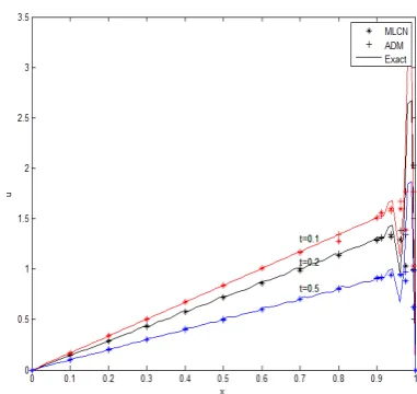
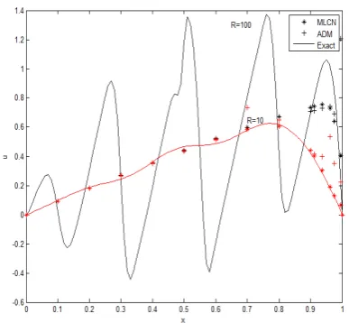
Figure 1: Comparison of the analytical method and the ADM and MLCN in the three steps of timet= 0.1,0.2,0.5 forR= 100.
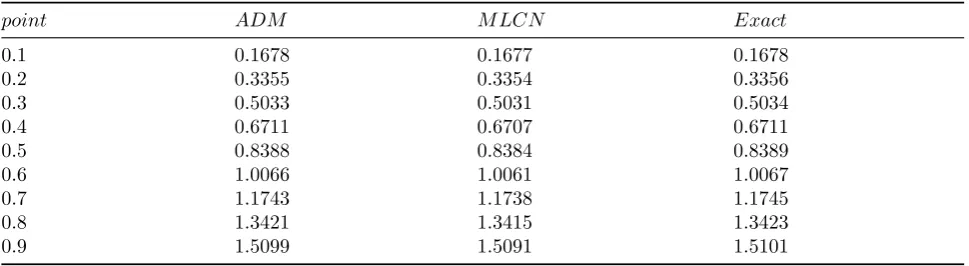
Table 1: The ADM and MLCN compared to the analytical solution of the R = 100 andτ= 10−4 andt= 0.1.
point ADM M LCN Exact
0.1 0.1678 0.1677 0.1678
0.2 0.3355 0.3354 0.3356
0.3 0.5033 0.5031 0.5034
0.4 0.6711 0.6707 0.6711
0.5 0.8388 0.8384 -0.8389
0.6 1.0066 1.0061 1.0067
0.7 1.1743 1.1738 1.1745
0.8 1.3421 1.3415 1.3423
0.9 1.5099 1.5091 1.5101
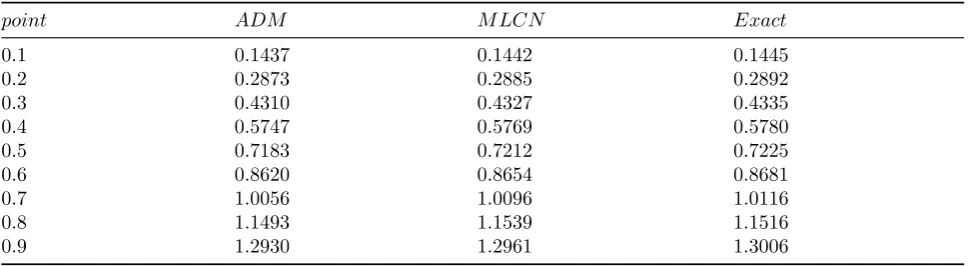
Table 2: The ADM and MLCN compared to the analytical solution of the R = 100 andτ= 10−4 andt= 0.2.
point ADM M LCN Exact
0.1 0.1437 0.1442 0.1445
0.2 0.2873 0.2885 0.2892
0.3 0.4310 0.4327 0.4335
0.4 0.5747 0.5769 0.5780
0.5 0.7183 0.7212 0.7225
0.6 0.8620 0.8654 0.8681
0.7 1.0056 1.0096 1.0116
0.8 1.1493 1.1539 1.1516
0.9 1.2930 1.2961 1.3006
Table 3: The ADM and MLCN compared to the analytical solution of the R = 100 andτ= 10−4 andt= 0.5.
point ADM M LCN Exact
0.1 0.1004 0.1012 0.1020
0.2 0.2008 0.2027 0.2041
0.3 0.3012 0.3040 0.3061
0.4 0.4016 0.4053 0.4082
0.5 0.5020 0.5066 0.5102
0.6 0.6024 0.6080 0.6122
0.7 0.7028 0.7093 0.7143
0.8 0.8032 0.8106 0.8163
0.9 0.9036 0.9117 0.9184
Table 4: The ADM and MLCN compared to the analytical solution of the R = 10 andτ= 10−4 andt= 0.1.
point ADM M LCN Exact
0.1 0.1678 0.1677 0.1678
0.2 0.3355 0.3354 0.3356
0.3 0.5033 0.5031 0.5034
0.4 0.6711 0.6707 0.6711
0.5 0.8388 0.8384 0.8389
0.6 1.0066 1.0061 1.0067
0.7 1.1743 1.1738 1.1745
0.8 1.3421 1.3415 1.3423
Table 5: The ADM and MLCN compared to the analytical solution of the R = 10 andτ= 10−4 andt= 0.2.
point ADM M LCN Exact
0.1 0.1437 0.1442 0.1445
0.2 0.2873 0.2885 0.2892
0.3 0.4310 0.4327 0.4335
0.4 0.5747 0.5769 0.5780
0.5 0.7183 0.7212 0.7225
0.6 0.8620 0.8654 0.8681
0.7 1.0056 1.0096 1.0116
0.8 1.1493 1.1539 1.1516
0.9 1.2930 1.2961 1.3006
Table 6: The ADM and MLCN compared to the analytical solution of the R = 10 andτ= 10−4 andt= 0.5.
point ADM M LCN Exact
0.1 0.1004 0.1012 0.1020
0.2 0.2008 0.2027 0.2041
0.3 0.3012 0.3040 0.3061
0.4 0.4016 0.4053 0.4082
0.5 0.5020 0.5066 0.5102
0.6 0.6024 0.6080 0.6122
0.7 0.7028 0.7093 0.7143
0.8 0.8032 0.8106 0.8163
0.9 0.9036 0.9117 0.9184
Table 7: The ADM and MLCN compared to the analytical solution of the R = 80 andτ= 10−4 andt= 0.1.
point ADM M LCN Exact
0.1 0.1678 0.1677 0.1678
0.2 0.3355 0.3354 0.3356
0.3 0.5033 0.5031 0.5034
0.4 0.6711 0.6707 0.6711
0.5 0.8388 0.8384 0.8389
0.6 1.0066 1.0061 1.0067
0.7 1.1743 1.1738 1.1745
0.8 1.3421 1.3415 1.3423
0.9 1.5099 1.5091 1.5101
Table 8: The ADM and MLCN compared to the analytical solution of the R = 80 andτ= 10−4 andt= 0.2.
point ADM M LCN Exact
0.1 0.1437 0.1442 0.1445
0.2 0.2873 0.2885 0.2892
0.3 0.4310 0.4327 0.4335
0.4 0.5747 0.5769 0.5780
0.5 0.7183 0.7212 0.7225
0.6 0.8620 0.8654 0.8681
0.7 1.0056 1.0096 1.0116
0.8 1.1493 1.1539 1.1516
Table 9: The ADM and MLCN compared to the analytical solution of the R = 80 andτ= 10−4 andt= 0.5.
point ADM M LCN Exact
0.1 0.1004 0.1012 0.1020
0.2 0.2008 0.2027 0.2041
0.3 0.3012 0.3040 0.3061
0.4 0.4016 0.4053 0.4082
0.5 0.5020 0.5066 0.5102
0.6 0.6024 0.6080 0.6122
0.7 0.7028 0.7093 0.7143
0.8 0.8032 0.8106 0.8163
0.9 0.9036 0.9117 0.9184
Table 10: The ADM and MLCN compared to the analytical solution of the R = 100 andτ= 10−4andt= 0.1.
point ADM M LCN Exact
0.1 0.0906 0.0916 0.0240
0.2 0.1802 0.1814 0.3076
0.3 0.2680 0.2703 0.2322
0.4 0.3531 0.3572 0.1931
0.5 0.4345 0.4313 1.1852
0.6 0.5114 0.5218 0.1884
0.7 0.5831 0.5983 0.8068
0.8 0.6488 0.6700 0.4066
0.9 0.7079 0.7361 0.4217
Table 11: The ADM and MLCN compared to the analytical solution of the R = 100 andτ= 10−4andt= 0.2.
point ADM M LCN Exact
0.1 0.0819 0.0834 0.0488
0.2 0.1629 0.1663 0.1747
0.3 0.2423 0.2482 0.4250
0.4 0.3192 0.3286 0.1156
0.5 0.3928 0.4070 0.5927
0.6 0.4624 0.4829 0.4232
0.7 0.5272 0.5557 0.4056
0.8 0.5867 0.6250 0.8655
0.9 0.6402 0.6898 0.4710
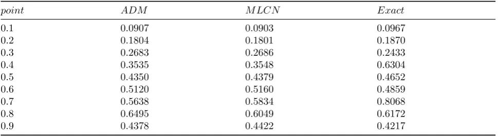
Table 12: The ADM and MLCN compared to the analytical solution of the R = 10 andτ= 10−4 andt= 0.1.
point ADM M LCN Exact
0.1 0.0907 0.0903 0.0967
0.2 0.1804 0.1801 0.1870
0.3 0.2683 0.2686 0.2433
0.4 0.3535 0.3548 0.6304
0.5 0.4350 0.4379 0.4652
0.6 0.5120 0.5160 0.4859
0.7 0.5638 0.5834 0.8068
0.8 0.6495 0.6049 0.6172
Table 13: The ADM and MLCN compared to the analytical solution of the R = 10 andτ= 10−4 andt= 0.2.
point ADM M LCN Exact
0.1 0.0820 0.0823 0.0828
0.2 0.1631 0.1642 0.1635
0.3 0.2426 0.2451 0.2431
0.4 0.3191 0.3241 0.3234
0.5 0.3932 0.3996 0.4001
0.6 0.4629 0.4671 0.4649
0.7 0.5278 0.5095 0.5034
0.8 0.5873 0.4815 0.4755
0.9 0.4409 0.3140 0.3115
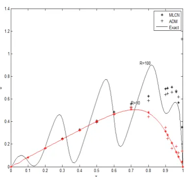
Figure 3: Comparison of the analytical method and the ADM and MLCN in the three steps of timet= 0.1,0.2 and 0.5 forR= 80.
4
The
modified
local
Crank-Nicolson method and
Analyt-ical solution for one
dimen-tional Bergur’s solution
4.1 The modified local Crank-Nicolson method
The Crank-Nicolson method (CN) is a central finite difference method. It should be noted that the Crank-Nicholson method is an implicit method, to obtain the values of u in the next steps, a set of algebraic equations must be solved, because the partial differential values are non-linear. Therefore, the discretization of these values must be non-linear. For many Burgers equations and many other equations it can be shown that the Crank-Nicholson method is un-conditional stable. The modified local
Crank-Figure 4: Comparison of analytical method and the MLCN and ADM with Reynolds numbers 10 and 100 in time stept= 0.1.
Nicholson method (MLCN) converts the partial differential equations into ordinary differential equations. The MLCN converts Coefficients ma-trixes into simple block mama-trixes. Using the Hopf - Cole conversion or using other conversion, the Burgers nonlinear equation becomes a linear equation [24], To solve equation (1) with the given boundary conditions using the central difference the following discretization equation is achieved [24].
dV(t)
dt =
1
2h2AV(t). (4.21)
Where the vector V(t) represents approximate
u values in the Burgers equation (1), h is the spatial step, ∆t is the time step and A is a tree diagonal matrix with dimensions (M − 1) × (M − 1) . Then the by inte-grating equation (21) and defininge the vector
Figure 5: Comparison of the analytical method and the MLCN and ADM with Reynolds numbers 10 and 100 in time stept= 0.2.
we will have:
V(tn+1) = exp (
∆t
2h2A )
V(tn). (4.22)
However, the Crank-Nicholson method for the Burgers equation (1) gives the following result:
V(tn+1) = (
(1−λA)−1))((1 +λA))V(tn).
(4.23) Where λ = 4τh2 is called the networking ratio.
The following equation is obtained by comparing equations (22) and (23):
exp
(
∆t
2h2A )
≈((1−λA)−1))((1 +λA)).
4.2 Analytical solution
The non-linear equation is given as [27]:
Lu(t) +N u(t) =g(t). (4.24)
Where L is a linear operator, N a nonlinear operator, andg(t) is a known analytical function. According to the variational iteration method (VIM) we can have the following recursive relation:
un+1(x, t) =un(x, t) +
∫ t
0
λ(ξ)(Lun(ξ)
+Nubn(ξ)−g(ξ))dξ (4.25)
Whereλis the general Lagrange multiplier which can be identified by the variational theory. Is
an initial u0(t) approximation that may be
un-known. Andbunis considered as boundary change
and δbun = 0 . Thus, in the first iteration of the
Lagrange multiplier λ is characterized which is obtained using fractional integration. Successive approximations un+1(t), are for the solution of
u(t) which is easily obtained using the Lagrange multiplier and using any selective functions u0 .
Consequently, the exact solution can be achieved using u= limn7→∞un.
Equation (1) with initial and boundary condi-tions is considered, for solving Eq. (1) with initial condition (2), via VIM, And with replacement in (26), it is written in the form of the original equa-tion [27] .
un+1(x, t) =un(x, t)
+
∫ t
0
λ(ξ)(∂un
∂ξ (x, ξ)
+bun ∂bun
∂x (x, ξ)
−ν∂
2ub n
∂x2 (x, ξ))dξ (4.26)
To make this correction functional stationary,
δun(x,0) = 0 having we derive:
δun+1(x, t) =δun(x, t)
+
∫ t
0
λ(ξ)(δun(x, ξ))
′
dξ. (4.27)
Its stationary conditions can be determined as follows:
λ′(ξ) = 0 1 +λ(ξ)|ξ=t= 0
From which the Lagrange multiplier can be iden-tifiedλ=−1, and the following iteration formula is obtained:
un+1(x, t) =un(x, t)
−
∫ t
0
(∂un
∂ξ (x, ξ) +un ∂un
∂x (x, ξ)
−ν∂
2u n
∂x2 (x, ξ))dξ (4.28)
Beginning with u0 =u(x,0) =f(x) the
boundary conditions (2) by VIM we have:
un+1(x, t) =un(x, t)
+
∫ t
0
λ(η)(∂un
∂ξ (η, t)
+ubn ∂ubn
∂x (η, t)
−ν∂
2bu n
∂x2 (η, t))dη. (4.29)
To find the optimal value ofλ, havingδun(0, t) =
0 leads to:
δun+1(x, t) =δun(x, t)−νδu
′
n(η, t)|x0 −λ′(η)(δun(η, t))|x0
+
∫ t
0
λ”(η)(δun(η, t))dη. (4.30)
Therefore, the stationary conditions are obtained as:
λ”(η) = 0
1 +νλ′(η)|η=x= 0
λ(η)|η=x= 0
This results in λ(η) = 1ν(x −η) and a desired iterative relation can be constructed as:
un+1(x, t) =un(x, t)
+1
ν
∫ t
0
(x−η)(∂un
∂ξ (η, t)
+un ∂un
∂x (η, t)
−ν∂
2u n
∂x2 (η, t))dη. (4.31)
Beginning with theu0 =f1(t)+xf2(t) an
approx-imate solution of (1) can be determined via the iterative formula (31).
5
Numerical examples
Problem 1. In this example, the numerical so-lution of the Burgers equation using the ADM and the MLCN and the comparison between the result and the analytical solution is given [27]
u(x, t) = 2x 1 + 2t
The above equation for t = 0 has its own initial conditions. With initial and boundary conditions
for t, and changing t, we solve the Eq. In this example, the length of time step τ = 0.004 and the node hx = 0.0125 but t changes:
u(x,0) = 2x.
uni,0 = 0.025×i.
uni,1 =− 0.05×i (1 + 2(n+ 1)0.004)2
uni,2 =
(
−0.1×i×(2 + 2(n+ 1)0.004)2 (1 + 2(n+ 2)0.004)2
)
× (
1
(1 + 2(n+ 1)0.004)2 )
And finallyuni comes in the form below:
uni ≈uni,0+uni,1+uni,2.
In this example, the greater the Reynolds number, the closer the Adomian answer to the analytical solution answers (See Figure 1 and Table 1, 2, 3), and the smaller the Reynolds number, the closer the MLCN answer to the an-alytical solution answer (See Figure 2 and Table 4, 5, 6), and if t is smaller the Adomian answer is more precise, so in any Reynolds number if t is considered very small, the Adomian method can be more accurate than the MLCN (See Figure 3 and Table 7,8,9) .
Problem 2. In this example, the numerical so-lution of the Burgers equation using the ADM and the MLCN and the comparison of the result to the analytical solution results are given:
u(x, t) =e−tsin(x).
The above equation for t = 0 has its own initial conditions. With the initial and boundary condi-tions for t, and changing t, we solve Eq. In this example, the length of time step τ = 0.004 and the node hx = 0.0125 but t changes:
u(x,0) = sin(x).
13), but in such functions the MLCN works bet-ter than the ADM method in larger t amounts and with smaller Reynolds numbers the answer is more precise .
6
Discussion and conclusion
The Burgers equation is a mix of convection and diffusion sentences, and is a simplified form of the Navier-Stockes equation. The Adomian numerical decomposition method has been pre-sented for solving the one-dimensional Burgers equations and has been compared to the modi-fied Local Crank-Nicolson numerical method, and the results of the two methods have been com-pared to the results of the analytical method. MLCN method is an explicit unconditional sta-bility. Two examples with different initial condi-tions have been solved and the accuracy of the solution methods ADM and MLCN in different Reynolds numbers has been studied. It has been observed that in Trigonometric functions with smaller Reynolds numbers and larger t amounts the MLCN method behaves better than the ADM method.
References
[1] H. Bateman, Some recent researches on the
motion of fluids, Mon. Weather Rev, 43
(1915) 163-170.
[2] M. Beck, Burgers Equation. Department of Mathematics, (2012) 1-4.
[3] H. Aminikhah, An analytical approximation for coupled viscous Burgers equation, Appl. Math. Modelling, 37 (2013) 5979-5983.
[4] A.H. Salas, Symbolic computation of solu-tions for a forced Burgers equation, Appl. Math. Comput, 216 (2010) 18-26.
[5] A.M. Wazwaz,Multiple soliton solutions and rational solutions for the (2+1)-dimensional dispersive long waterwave system, Ocean En-gineering, 60 (2013) 95-98.
[6] C.Q. Dai, and F.B. Yu, Special solitonic localized structures for the one-dimensional Burgers equation in water waves, Wave Mo-tion, 51 (2014) 52-59.
[7] J. Zhou,Novel soliton-like and multi-solitary wave solutions of (3+1)-dimensional
Burg-ers equation, Appl. Math. Comput, 204
(2008) 461-467.
[8] A.M. Wazwaz, A study on the one-dimensional and the two-one-dimensional higher-order Burgers equations, Appl. Math. Let-ters, 25 (2012) 1495-1499.
[9] F. Kong, and S. Chen,New exact soliton-like solutions and special soliton-like structures of the (2+1) dimensional Burgers equation, Chaos, Solitons and Fractals, 27 (2006) 495-500.
[10] E. Demetriou, M.A. Christou, and C. Sopho-cleous,On the classification of similarity so-lutions of a two-dimensional
diffusionadvec-tion equadiffusionadvec-tion , Appl. Math. Comput, 187
(2007) 1333-1350.
[11] G. Zhao, X. Yu, and R. Zhang, he new nu-merical method for solving the system of two-dimensional Burgers equations, Appl. Math. Comput, 62 (2011) 3279-3291.
[12] M.A. Christou, and C. Sophocleous, Nu-merical similarity reductions of the (1+3)-dimensional Burgers equation ,Appl. Math. Comput, 217 (2011) 7455-7461.
[13] W. Liao, An implicit fourth-order compact finite difference scheme for one-dimensional Burgers equation, Appl. Math. Comput, 206 (2008) 755-764.
[14] A.H.A.E. Tabatabaei, E. Shakour, and M. Dehghan,Some implicit methods for the nu-merical solution of Burgers equation, Appl. Math. Comput, 191 (2007) 560-570.
[15] H. Chen, and Z. Jiang, A characteristics-mixed finite element method for Burgers equation. Korean , Appl. Math. Comput. J. 15 (2004) 29-51.
[16] J. D. Cole, On a Quasi-Linear Parabolic Equation Occurring in Aerodynamics,Quart. Appl. Math. 9 (1951) 225-236.
[18] S. Abbasbandy, M. T. Darvishi, A numeri-cal solution of Burgers equation by modified
Adomian method, Appl. Math. Comput. 163
(2005) 1265-1272.
[19] H. Zhu, H. Shu, M. Ding, Numerical solu-tions of two-dimensional Burgers equasolu-tions by discrete Adomian decomposition method, Appl. Math. Comput. 60 (2010) 840-848.
[20] G. Adomian, Application of the decomposi-tion method to the Navier-Stokes equadecomposi-tions, Appl. Math. Analytic. J. 119 (1986) 340-360.
[21] A. M. Abduwali, A corrector local C-N method for the two-dimensional heat equa-tion), Math. Numer. Shin. 19 (1997) 267-276.
[22] A. M. Abduwali, M. Sakakihara, and H. Niki, A local Crank-Nicolson method for solving the heat equation , Hiroshima Math. J. 24 (1994) 1-13
[23] A. M Wazwaz,A (3+1)-dimensional nonlin-ear evolution equation with multiple soliton solutions and multiple singular soliton
so-lutions , Appl. Math. Comput. 215 (2009)
1548-1552.
[24] P. Huang, A. Abduwali, The Modified Lo-cal Crank-Nicolson method for one- and two-dimensional Burgers equations, Appl. Math. Comput. 59 (2010) 2452-2463.
[25] E. R. Benton, G. W. Platzman,A table of so-lutions of the one-dimensional Burgers equa-tion , Quarterly of Appl. Math 30 (1972) 195-216.
[26] A. R. Bahadr, A fully implicit finite-difference scheme for two-dimensional
Burg-ers equations , Appl. Math. Comput. 137
(2003) 131-137.
[27] J. H. A. Biazar, Exact and numerical so-lutions for non-linear Burgers equation by VIM, Math. Comput. Modelling 49 (2009) 1394-1400.
Ahmad Reza Haghighi is an Assis-tant Professor in the department of mathematics at Urmia Univer-sity of technology, Urmia, Iran. He completed his Ph. D degree in ap-plied mathematics from Pune Uni-versity, India. His research in-terest includes Bio-Mathematics, Computational Fluid Dynamics, Partial Differential Equations and Control