VOLUME 41, ARTICLE 15, PAGES 425
-
460
PUBLISHED 31 JULY 2019
https://www.demographic-research.org/Volumes/Vol41/15/ DOI: 10.4054/DemRes.2019.41.15
Research Article
Is the age difference between partners related to
women’s earnings?
Angela Carollo
Anna Oksuzyan
Sven Drefahl
Carlo Giovanni Camarda
Linda Juel Ahrenfeldt
Kaare Christensen
Alyson van Raalte
© 2019 Angela Carollo et al.
This open-access work is published under the terms of the Creative Commons Attribution 3.0 Germany (CC BY 3.0 DE), which permits use, reproduction, and distribution in any medium, provided the original author(s) and source are given credit.
1 Introduction 426
2 Background 429
2.1 Gender gap in pay 429
2.2 Reasons for age gaps in marriage 430
3 Data and methods 431
3.1 Data 431
3.2 Variables 432
3.3 Statistical analysis 433
4 Results 434
4.1 Descriptive results 434
4.2 Within-twin comparisons 435
4.3 Unconditional quantile regression model 437
5 Discussion 442
References 449
Is the age difference between partners related to women’s earnings?
Angela Carollo1
Anna Oksuzyan2
Sven Drefahl3
Carlo Giovanni Camarda4
Linda Juel Ahrenfeldt5
Kaare Christensen5 Alyson van Raalte2
Abstract
BACKGROUND
Women earn less than men at most career stages. Explanations for a gender gap in wages include gender differences in the allocation of household and domestic work. At the family level, a marital age difference is an important shared characteristic that might play a role in determining a woman’s career trajectory, and, therefore, her income. Since women tend to marry older men, we investigate whether women whose husbands are older have lower incomes than women whose husbands are the same age or younger.
OBJECTIVE
This study investigates whether the age gap between a woman and her partner was associated with her income in Denmark in 2010.
METHODS
We use data on Danish female twin pairs in 2010. Our design includes samples within twin pairs (n = 4,716) and pooled twin samples (n = 13,354) to account for differences in early household environments and uses unconditional quantile regression to model the association between the age gap and the woman’s income.
1 Max-Planck-Institut für Demografische Forschung, Rostock, Germany. Email:[email protected]. 2 Max-Planck-Institut für Demografische Forschung, Rostock, Germany.
3 Stockholms Universitet, Sweden.
RESULTS
We find a statistically significant association between the marital age gap and the woman’s income. The form of this association appears to be complex and varies across the income and age gap distribution. However, the magnitude of the estimated effects is small in economic terms.
CONCLUSIONS
These results suggest that the marital age gap is unlikely to be an important determinant of a woman’s income, at least in Denmark.
CONTRIBUTION
To our knowledge, this is the first study that explores the association between marital age differences and a woman’s earnings using a twin design and high-quality register data.
1. Introduction
The gender gap in income is large and persists throughout the life course. In the 28 countries of the European Union in 2014, the average gender wage gap (the difference between the average gross hourly earnings of male and of female paid employees as a percentage of the average gross hourly earnings of male paid employees) was about 16.7% (Eurostat 1994–2014). Men out-earn women starting with their entry into the labor market, and gender differences in pay increase with age (Eurostat 2008).
A substantial body of research has investigated the reasons for the gender differences in labor market outcomes in general, and in the gender wage gap in particular. In addition to examining gender segregation into educational fields and labor market segments, the existing theoretical work has focused primarily on gender differences in the allocation of household work and family responsibilities. This body of work includes theoretical accounts of relative resource bargaining (Blood and Wolfe 1960), household specialization (Becker 1981), as well as the ‘doing gender’ hypothesis (West and Zimmerman 1987).
power within the relationship, as well as the pathways toward specific forms of household specialization.
Women tend to marry men who are, on average, two to three years older (Buss 1989). Since income tends to rise with age, the male partner is likely to contribute more to the household’s economic resources than the female partner simply by virtue of being older (Rothstein 2012). At least in the short term, the best strategy the partners can use to maximize their household income is to optimize the income and the career prospects of the older, higher-earning male partner at the potential expense of the younger female partner. It follows that, on average, a woman with an older partner may be more willing to compromise her own career trajectory than a woman with a partner who is the same age or younger, which would be reflected in a negative association between the male and female marital age gap and the woman’s earnings.
For example, in academia, seniority is closely linked to stable employment opportunities for both men and women. Previous research has pointed out that couples pursuing dual careers in science face difficulties and that, in particular, women are less likely than men to secure a tenure-track position due to family constraints (Ackers 2004; Wolfinger, Mason, and Goulden 2009). Anecdotal evidence of dual-earner couples in the authors’ own social networks suggests that the partner who is older and who obtained his or her PhD first is also almost always the first to secure stable employment. In nearly all cases, this is the man. We wondered whether this pattern could be generalized, and whether examining the marital age gap can add important insights about career trajectories, particularly for women.
We expect to find that the association between a spousal age gap and the woman’s income varies across the female income distribution. A woman with a high income might be less willing to sacrifice her own career regardless of whether her partner is older, which would result in a null association between the age gap and the woman’s earnings. On the other hand, a woman with a low income may be more likely to compromise her own career in order to help her partner advance. In this case, we would expect to see a negative association between the spousal age gap and the woman’s earnings. It is, however, possible that higher-income couples have greater agency in defining their career paths and the number of hours worked, which would result in a stronger association between the age gap and the woman’s income for high-income women.
older man is expected to take on a larger share of the household responsibilities because her husband is from a birth cohort with more traditional gendered values. These expectations could lead her to reduce her working hours, which has a direct dampening effect on her wages, and which again results in a negative association between the spousal age gap and the woman’s income.
Finally, a large age gap in a relationship in which the man is older could indicate that the couple has formed a more patriarchal household in which the man is expected to have a more established and successful career than the woman. Consequently, a woman who partners with an older man might be directly or indirectly signaling a willingness to take on a greater share of the domestic duties, while the man in such a couple may expect to take on fewer household responsibilities.
There are also a number of reasons to assume that marital age differences affect women’s earnings only slightly or not at all. For example, the effect of a spousal age gap on a woman’s earnings can be short-lived. Kahn, García-Manglano, and Bianchi (2014) showed that motherhood reduces women’s labor force participation at younger ages only, and that the effect disappears later in the life course, when women are in their forties and fifties. Alternatively, a woman may start to invest more in her career after her husband has reached the desired level in his career. Finally, given these many factors that may disrupt the link between a marital age gap and the woman’s earnings, it is worth emphasizing that this relationship may have no clear causal path.
To date, studies that have investigated the impact of a spousal age gap on earnings have found that women who marry men men of similar age out-earn women who marry older men (Dribe and Nystedt 2017; Mansour and McKinnish 2014). In their analysis of how the earnings of Swedish women change before and after partnership formation, Dribe and Nystedt (2017) found that wage differences based on the marital age gap were already present prior to union formation. Thus, the authors attributed this pattern to selection through assortative mating rather than characterizing it as a true causal effect. This suggests either that the theory that partnering with an older man reduces a women’s income is wrong, or that other pathways are present. For instance, the degree of patriarchy in an individual’s early childhood environment might be expected to affect his or her partnership formation behavior and degree of career orientation.
quantiles. Finally, we separately analyze younger and older birth cohorts based on secular differences in the division of household labor.
2. Background
2.1 Gender gap in pay
In the 20th century, it was posited that a substantial share of the male to female wage differential can be explained by differences in occupational qualifications upon entry into the labor market, and that these differences were important determinants of future wage prospects (Blau and Kahn 2000; Kunze 2005). However, even though the educational attainment of women has increased considerably in recent years, with women having higher educational qualifications than men in many countries, the gender wage gap persists in all countries (Eurostat 1994–2014).
Comparative international studies have suggested that the gender wage gap is influenced by wage structures, i.e., “prices determined for labor market skills and the rewards to employment in particular sectors” (Blau and Kahn 2000: 6). Rosholm and Smith (1996) argued that differences in wage dispersion in the private vs. the public sector, which employs higher proportions of women, helps to explain the gender wage gap in Denmark.
Some empirical analyses have investigated how noncognitive traits affect gender wage differentials (Fortin 2008). Studies conducted in Sweden and the Netherlands have suggested that women are less likely to negotiate for higher compensation and respond differently to negotiation outcomes (Säve-Söderbergh 2007; Wahlberg 2010). It has also been argued that women tend to have work-related preferences other than compensation that cause them to have lower wages than men (Fransen, Plantenga, and Vlasblom 2012).
In Denmark, the adoption of the principle of equality of pay for men and women in 1973, and the enforcement of this principle by the European Union starting in 1976, led to a reduction in the gender pay gap in the 1970s (Rosholm and Smith 1996). Although this trend plateaued in the 1980s, at least in the private sector, Denmark continued to have a smaller gender pay gap than the Netherlands, Germany, Ireland, the United Kingdom, and the United States until the early 1990s. In 2014, the average Danish woman earned 16.0% less than the average Danish man, a figure that is only slightly below the EU-28 average (16.6%) (Eurostat 1994–2014). When other domains of gender equality are considered, Denmark is found to be among the leading EU countries. In the Gender Equality Index, which measures gender gaps adjusted for achievement levels, Denmark is ranked third after Sweden and Finland (EIGE 2015). In the United Nation’s Gender Inequality Index, Denmark is ranked fourth out of the 155 countries included, in part because it has very low levels of inequality in domains such as reproductive health and empowerment (Jahan et al. 2015). The country’s role as one of the EU leaders in gender equality makes Denmark a good setting for investigating the possible relationship between the spousal age gap and income because this relationship is not distorted by gender differences in labor market outcomes.
2.2 Reasons for age gaps in marriage
Both currently and historically, the male partner is older than the female partner in the majority of marital unions (Gustafson and Fransson 2015). Although it has been shown that the mean age at marriage increased in many developed and developing countries over the 20th century (Billari 2005), trends in spousal age differences have received less
attention. The average marital age gap in Denmark was 2.8 years in 2010 (Statistics Denmark 2010) and remained relatively stable throughout the 20th century (Drefahl
2010a).
It has also been suggested that gender equality, the status of women, and gender-related social norms are important determinants of cross-national variation in age differences at marriage. Comparative studies have shown that the age gap is larger in developing countries with more traditional gender roles than in countries with higher levels of gender equality (Casterline, Williams, and McDonald 1986). Social norms may also contribute to the spousal age gap distribution (Presser 1975). Generally, it is more socially acceptable for a woman to marry an older man than a younger man, and a large age discrepancy in a partnership is viewed negatively when the man is older, and especially when the woman is older (Banks and Arnold 2001).
Previous empirical research has indicated that having low levels of education and income, being unemployed, and having a migration background are associated with larger spousal age differences (Atkinson and Glass 1985; Gustafson and Fransson 2015; Vera, Berardo, and Berardo 1985).
3. Data and methods
3.1 Data
The Danish Twin Registry is the world’s oldest national twin register, and it contains information on more than 86,000 twin pairs born in Denmark since 1870 (Skytthe et al. 2013).
The present study utilizes the Central Person Register (CPR) (since 1968), the Danish Twins Register (since 1954), the Integrated Database for Labor Market research (IDA) (since 1980), and the Population Education Register (PER) (since 1981), which were linked using 10-digit unique personal identification numbers (Baadsgaard and Quitzau 2011; Pedersen 2011; Petersson, Baadsgaard, and Thygesen 2011; Skytthe et al. 2013).
We employ a twin design to control for differences in the early household environment and social development, which may be related to both income prospects and marriage, and which are often unobserved. For instance, some twin pairs may come from patriarchal families that encourage both large marital age gaps and low levels of female autonomy, whereas other twin pairs may come from more egalitarian households. These differences would not be fully captured by traditional socioeconomic controls such as parental education. Moreover, without using a twin design, unobserved family characteristics could be correlated with such traditional controls.
endowments. In addition to having similar genetic characteristics, twins who are raised together experience similar social and economic conditions during childhood and adolescence. Thus, studying twins provides us with a unique opportunity to gain a better understanding of how genetic and early social environments affect behaviors and choices in later stages of life (Kohler, Behrman, and Schnittker 2011).
The study is based on all female twin pairs born between 1945 and 1990 who were alive and resident in Denmark in 2010. We perform a within-pair analysis in which individuals are included only if both the individual and her twin were alive and married in 2010 (n = 4,716). Hereafter, we refer to these cases as complete twin pairs. We then perfom a pooled analysis to increase the size of the population (n = 13,354), although the advantages of the twin design are lost. The pooled analysis also includes incomplete twin pairs, such as cases in which one twin was unmarried or deceased in 2010. While it would have been desirable to include the entire Danish population in the pooled analysis, information on childbearing is not available from the general population registry, which is a critical determinant of female income.
We restrict the sample to women born after 1945 because there were major structural changes in women’s career and family situations in Denmark around the early 1960s (Grunow 2004). Prior to that time, it was uncommon for a married woman to engage in paid work. Same-sex couples are excluded from the analysis because our main focus is on gender relations.
3.2 Variables
We identify taxable gross income before deductions as the outcome of interest, converting the data from Danish krone into US dollars (on April 15, 2016, a Danish krona, 1DKK, was equal to around 0.15 US dollars). This indicator includes income from the following sources: wage income, retirement income, transfers from public monies, capital income, and income from abroad. Gross income is registered annually, and we extract the value registered in the year 2010. We decided to use gross income as the outcome of interest because it also allows us to retrieve information on retired women and women whose main sources of income are independent work, capital income, and/or transfers. We have chosen to include retired women even though they are no longer working because retirement income is based on previous work-related income, which may be associated with a marital age gap.
children, and some socioeconomic characteristics of the spouse, such as gross income in 2010 and retirement status. The highest level of education attained is measured according to the International Standard Classification of Education (ISCED), which has seven categories for Denmark (Eurydice 2014, 2016). To avoid small numbers, we have grouped together the categories ISCED 1–2 and ISCED 5–6. The category ISCED 0 is not observed among the women in our study. The employment status is identified as employed, unemployed, and out of the labor force. Included in this third category are pensioners, students, early retirees, and other people who are not in the labor force. Retirement status is divided into four categories: not retired, retired, retired early, and early retirement beneficiary; the differences between the last three categories can be determined by looking at the age at retirement and the type of pension plan chosen by the individual. We use the same approach to identify the retirement status of the spouse. The number of children is included as a factor with four levels: zero, one, two, and three or more children. The income of the partner is measured as the gross income in 2010 and is assigned to one of four categories according to the income distribution in the population: low, medium-low, medium-high, and high. Finally, the birth cohort variable distinguishes between women born in 1945–1964 (older cohorts) and women born in 1965–1990 (younger cohorts). Restricting the analysis to observations with no missing values in the variables results in a final sample size of 13,354 individuals.
3.3 Statistical analysis
We employ the recently proposed Unconditional Quantile Regression (Firpo, Fortin, and Lemieux 2009), UQR, to quantify any differences in effects that the marital age gap and the other covariates might have on different quantiles of the income distribution. The UQR provides more interpretable results in the context of a target population because it marginalizes the effect of the covariate of interest over the distributions of the other covariates in the model (Borah and Basu 2013). A woman’s ranking in the income distribution might be different in the unconditional distribution than it is in the distribution conditional upon the covariates. The UQR coefficient is then interpreted as the effect of an additional year of age gap in each of the quantiles of the unconditional distribution of income, net of the effect of the other covariates, where the ranking of women’s wages is determined prior to the regression.
into an ‘older cohort’ subpopulation born in 1945–1964, who are likely to be retired or at advanced career stages, and a ‘younger cohort’ subpopulation born in 1965–1990. We then run the model for each of these cohort groupings based on five income quantiles; that is: = {0.10, 0.25, 0.50, 0.75, 0.90}.
We first present some descriptive results, including a within-twin pairs comparison. We then show the results of the model estimated first in the complete twin pairs, and second in the pooled sample.
All of the analyses are performed using R and the R-packageuqr (Nembrini 2017; R Core Team 2017). The within-pair results are presented, followed by the results of the pooled analysis on the extended population.
4. Results
4.1 Descriptive results
To obtain an initial picture of the relationships among the variables included in the analysis, we consider nine categories of age difference, following the study by Mansour and McKinnish (2014). Among the complete twin pairs, 23% had a partner who was one year younger or older, 13% had a partner who was one to two years older, 30% of the female twins had a partner who was two to five years older, and 12% had a partner who was five to eight years older (Table A-1). Among all twins, these percentages are almost identical (22%, 13%, 29%, 13%) (Table A-2). Around 50% of all twins had a partner who was at least two years older, and only 9% of female twins had a partner who was at least two years younger.
Table A-1 shows for the complete twin pairs the mean values and the standard errors computed for the variables age at marriage and age, and the distribution of the age gap conditional on the other variables included in the analysis (Table A-2 for all twins). In 2010, the mean age of the women in our population was 48 years, both for the complete pairs and for all twins. On average, the women who were older than their husbands married at higher ages.
married to older men, while only 40% of women with a high-income spouse had an age difference of more than two years. The findings are similar in the pooled sample of all twins (Table A-2).
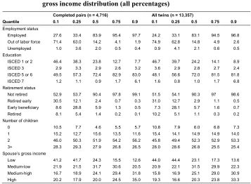
Table A-3 shows the characteristics of the women in each of the quantiles of the gross income distribution, for complete pairs and for all twins, to investigate the degree to which women differ in each part of the income distribution. Among the complete pairs of twins, medium-to-high earners were more likely to be employed, to be better educated (ISCED 5–6 and above), to have two children, and to have a spouse with a medium-high or high income. These findings signal a high degree of earning homogamy. The results for the pooled sample of all twins are similar.
4.2 Within-twin comparisons
We compute the absolute difference between the gross incomes of the two twins in each pair and plot the age gap of twin one against the age gap of twin two with the difference in their gross incomes added as a third variable. Different incomes are illustrated by different shades of blue (Figure 1). In Figure 1, dark dots indicate twin pairs with large income differences while bright dots indicate twin pairs with only small income differences.
Figure 1: Age gap of twin 1 versus age gap of twin 2
Note: Darker points indicate bigger absolute differences in gross income between twin one and twin two.
4.3 Unconditional quantile regression model
We first present the relationship between the marital age gap and the woman’s gross income estimated by the unconditional quantile regression model using a graph that compares the estimated curves (without intercept) for the two cohorts in the within-twin pairs sample (Figure 2).
Figure 2: Estimated curves for the effect of the marital age gap on the woman’s gross income; older cohort (left panel), younger cohort (right panel); within-twin pairs sample (n = 4,716)
Figure 2 shows that the relationship between the marital age gaps and the gross incomes of the twins in the complete-twin pairs is complex and varies in the different parts of the income distribution and in the different parts of the age gap distribution.
In the older cohort, increasingly negative age gaps (the wife is older than the husband) are associated with decreasing incomes for very low-income women (tau = 0.10), for middle-high-income women (tau = 0.75), and for high-income women (tau = 0.90). The relationship is first slightly decreasing and then slightly increasing for low-middle-income (tau = 0.25) and medium-income earners (tau = 0.50). The opposite pattern can be observed for positive age gaps (the husband is older than the wife), with the association between the age gap and income being almost null for low-income women (tau = 0.10) and medium-income earners (tau = 0.5), increasing for high-middle-income women (tau = 0.75), and first increasing and then decreasing for all other income groups.
Woman older Man older Woman older Man older
Old cohort Young cohort
–10 –5 0 5 10 –10 –5 0 5 10
–5000 –2500 0 2500 5000
Age gap
E
stima
ted
eff
e
c
t
o
n
in
c
om
e
The situation appears to be different in the younger cohort, for whom retirement effects are unimportant. Increasingly negative age gaps are associated with decreasing incomes for all income groups except the highest earners (tau = 0.90). In the middle-income to high-middle-income groups (tau = 0.5, tau = 0.75, and tau = 0.9), there is a negative association between positive increasing age differences and incomes; while in the low-income groups, this association is increasing (tau = 0.10) or slightly increasing and then flattening (tau = 0.25).
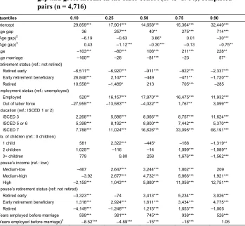
Table 1: Unconditional quantile regression for the association between the age gap and gross income in the older cohort (1945–1964); completed pairs (n = 4,716)
Quantiles 0.10 0.25 0.50 0.75 0.90
Intercept 29,859*** 17,901*** 14,658*** 15,364*** 32,440***
Age gap 36 257*** 40** 275*** 714***
(Age gap)2 –6.19 –0.63 3.86* 0.01 –30***
(Age gap)3 0.43 –1.12*** –0.30*** –0.13 –0.75**
Age –103*** –80*** 106*** 211*** 228**
Age marriage –160** –28 –81*** –23 57*
Retirement status (ref.: not retired)
Retired early –6,511** –6,920*** –911*** –822*** –2,337***
Early retirement beneficiary 26,848*** 2,147*** –449 –471** –1,720***
Retired 10,558** –1,489* 213 705*** –285
Employment status (ref.: unemployed)
Employed 520** 16,157*** 17,870*** 16,475*** 11,932***
Out of labor force –27,955*** –13,583*** –4,022*** 1,767** 3,099***
Education (ref.: ISCED 1 or 2)
ISCED 3 2,268*** 5,586*** 8,066*** 8,757*** 11,624***
ISCED 5 or 6 5,398*** 8,192*** 8,800*** 7,442*** 5,370***
ISCED 7 7,788*** 11,024*** 16,626*** 33,095*** 66,191***
No. of children (ref.: 0 children)
1 child 581 2,322*** –445* –166 –1,319**
2 children 1,025** –116 –14 1,099*** –1,089**
3+ children 779 9.80 258 1,676*** –1,562***
Spouse’s income (ref.: low)
Medium-low –467 2,647*** 3,244*** 1,802*** 209
Medium-high –3.92 2,677*** 4,732*** 5,866*** 1,921***
High –2,155*** 1,043*** 5,880*** 11,056*** 12,751***
Spouse’s retirement status (ref: not retired)
Retired early –3,323*** –74 3,413*** 5,234*** 3,026***
Early retirement beneficiary 1,318*** 2,924*** 1,611*** 3,434*** 4,775***
Retired –4,149*** –1,248*** 1,215*** 1,653*** –1,005
Years employed before marriage 599*** 381*** 745*** 938*** 526***
(Years employed before marriage)2 –8.52*** –4.89*** –15*** –18*** 1.05
It should be noted, however, that some of these relationships do not have any statistical significance, possibly due to the small sample size of the within-twin pair sample. We present the coefficients and the results of the t-test (p-values, robust SE obtained through bootstrap sampling, 2,000 samples) in Tables 1 and 2.
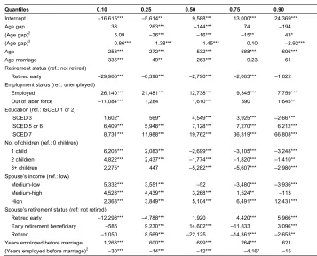
Table 2: Unconditional quantile regression for the association between the age gap and gross income in the younger cohort (1965–1990); completed pairs (n = 4,716)
Quantiles 0.10 0.25 0.50 0.75 0.90
Intercept –16,615*** –5,614** 9,588*** 13,000*** 24,369***
Age gap 38 263*** –144*** 74 –194
(Age gap)2 5.09 –36*** –16*** –15** 43*
(Age gap)3 0.86*** 1.38*** 1.45*** 0.10 –2.92***
Age 258*** 272*** 532*** 688*** 606***
Age marriage –335*** –49** –263*** 9.23 61
Retirement status (ref.: not retired)
Retired early –29,966*** –6,398*** –2,790*** –2,003*** –1,022
Employment status (ref.: unemployed)
Employed 26,140*** 21,481*** 12,738*** 9,345*** 7,759***
Out of labor force –11,084*** 1,284 1,610*** 390 1,645**
Education (ref.: ISCED 1 or 2)
ISCED 3 1,602* 569* 4,549*** 3,925*** –2,667**
ISCED 5 or 6 6,409*** 5,948*** 7,128*** 7,270*** 6,212***
ISCED 7 8,731*** 11,988*** 19,762*** 36,319*** 66,808***
No. of children (ref.: 0 children)
1 child 6,203*** 2,083*** –2,699*** –3,105*** –3,248***
2 children 4,822*** 2,437*** –1,774*** –1,820*** –1,410**
3+ children 2,275* 447 –5,282*** –5,607*** –2,980***
Spouse’s income (ref.: low)
Medium-low 5,332*** 3,551*** –52 –3,480*** –3,936***
Medium-high 4,528*** 4,439*** 3,268*** 1,524** –113
High 2,368*** 3,849*** 5,104*** 6,491*** 12,431***
Spouse’s retirement status (ref: not retired)
Retired early –12,298*** –4,788*** 1,920 4,420*** 5,966***
Early retirement beneficiary –585 9,230*** 14,602*** –11,833 3,096***
Retired –1,050 8,569*** –22,125 –14,361*** –2,653**
Years employed before marriage 1,268*** 600*** 699*** 264*** 621
(Years employed before marriage)2 –30*** –14*** –12*** –4.16* –15
Note: *p < .05. **p < .01. ***p < .001.
pairs analysis, we first present the estimated curves in Figure 3, and then show the coefficients in Table 3 (older cohorts) and Table 4 (younger cohorts).
Figure 3: Estimated curves for the effect of the marital age gap on the woman’s gross income; older cohort (left panel), younger cohort (right panel); pooled twin pairs sample (n = 13,354)
As in the case of the within-twin pairs sample, we find for the pooled sample that the relationship between the age gap and the gross income is complex and varies across the two cohorts and the income groups.
In the older cohort, increasingly negative age differences are associated with increasing incomes for the lowest-income group (tau = 0.10), with steeply decreasing incomes for medium (tau = 0.50) and high-middle incomes (tau = 0.75), and with slightly decreasing incomes for low-middle (tau = 0.25) and high incomes (tau = 0.90). Positive increasing age differences (the husband is older than the wife) are associated with incomes that are first slightly increasing and then decreasing for all income groups except the middle-high-income women, for whom instead the relationship seems to be steeply increasing.
In the younger cohort, the picture again is different. Both low-income and high-income women experience an increasing relationship, with the age differences expanding in both directions (negative and positive). Medium-income and middle-low-income earners experience a negative relationship, with the age differences expanding in both directions. Finally, the relationship between the age gap and income is decreasing steeply for increasingly negative age gaps and is increasing slightly for positive age gaps for women in the medium-high-income group (tau = 0.75).
Woman older Man older Woman older Man older
Old cohort Young cohort
–10 –5 0 5 10 –10 –5 0 5 10
–4000 –2000 0 2000
Age gap
E
stima
ted
eff
e
c
t
o
n
in
c
om
e
We also controlled for the effects of age, age at marriage, employment status, highest educational level attained, number of children, retirement status, total number of years employed before marriage, and the gross income and retirement status of the partner (Tables 3 and 4). All coefficients, together with p-values and confidence intervals, are presented in Tables 3 and 4.
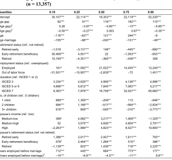
Table 3: Unconditional quantile regression for the association between the age gap and gross income in the older cohort (1945–1964); all twins (n = 13,357)
Quantiles 0.10 0.25 0.50 0.75 0.90
Intercept 30,107*** 22,114*** 16,353*** 22,119*** 52,230***
Age gap 82*** 91*** 116*** 182*** 110***
(Age gap)2 0.26 –3.87*** –3.60*** –13*** –5.85***
(Age gap)3 –0.50*** –0.27*** 0.003 0.67*** –0.35***
Age –116*** –63*** 121*** 244*** –9
Age marriage –155*** –88*** –240*** –131*** –49***
Retirement status (ref.: not retired)
Retired early –1,018 –3,131*** 148** –440** –690***
Early retirement beneficiary 30,469*** 4,501*** 22 –1,053*** –653***
Retired 10,190*** –4,351*** –365*** –438*** 308
Employment status (ref.: unemployed)
Employed 161* 11,092*** 21,022*** 14,455*** 12,240***
Out of labor force –31,501*** –15,957*** –2,839*** –72 1,451***
Education (ref.: ISCED 1 or 2)
ISCED 3 3,334*** 4,629*** 4,906*** 4,138*** 4,896***
ISCED 5 or 6 4,668*** 5,812*** 7,845*** 7,083*** 5,217***
ISCED 7 6,363*** 7,979*** 16,758*** 32,527*** 65,660***
No. of children (ref.: 0 children)
1 child 889*** 1,309*** –209** 113 –646**
2 children 894*** 1,166*** –517*** –564*** –2,834***
3+ children 816*** 859*** –545*** –310** –3,773***
Spouse’s income (ref.: low)
Medium-low 389* 4,082*** 3,217*** 1,009*** –1,325***
Medium-high 52 3,575*** 4,826*** 4,604*** 2,791***
High –2,263*** 1,999*** 4,823*** 8,527*** 10,800***
Spouse’s retirement status (ref: not retired)
Retired early 1,386*** 2,017*** 2,007*** 1,611*** 793**
Early retirement beneficiary 578* 2,464*** 1,284*** 515** 396**
Retired –1,139*** 823*** 1,436*** 718*** 2,225***
Years employed before marriage 712*** 445*** 684*** 773*** 177**
(Years employed before marriage)2 –14*** –6.8*** –4.5*** –11*** 8.8***
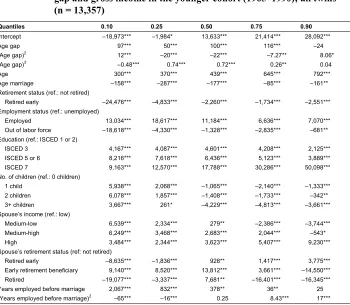
Table 4: Unconditional quantile regression for the association between the age gap and gross income in the younger cohort (1965–1990); all twins (n = 13,357)
Quantiles 0.10 0.25 0.50 0.75 0.90
Intercept –18,973*** –1,984* 13,633*** 21,414*** 28,092***
Age gap 97*** 50*** 100*** 116*** –24
(Age gap)2 12*** –20*** –22*** –7.27** 8.06*
(Age gap)3 –0.48*** 0.74*** 0.72*** 0.26** 0.04
Age 300*** 370*** 439*** 645*** 792***
Age marriage –158*** –287*** –177*** –85*** –161**
Retirement status (ref.: not retired)
Retired early –24,476*** –4,833*** –2,260*** –1,734*** –2,551***
Employment status (ref.: unemployed)
Employed 13,034*** 18,617*** 11,184*** 6,636*** 7,070***
Out of labor force –18,618*** –4,330*** –1,328*** –2,835*** –681**
Education (ref.: ISCED 1 or 2)
ISCED 3 4,167*** 4,087*** 4,601*** 4,208*** 2,125***
ISCED 5 or 6 8,216*** 7,618*** 6,436*** 5,123*** 3,889***
ISCED 7 9,163*** 12,570*** 17,788*** 30,286*** 50,098***
No. of children (ref.: 0 children)
1 child 5,938*** 2,068*** –1,065*** –2,140*** –1,333***
2 children 6,078*** 1,857*** –1,408*** –1,733*** –342**
3+ children 3,667*** 261* –4,229*** –4,813*** –3,661***
Spouse’s income (ref.: low)
Medium-low 6,539*** 2,334*** 279** –2,386*** –3,744***
Medium-high 6,249*** 3,468*** 2,683*** 2,044*** –543*
High 3,484*** 2,344*** 3,623*** 5,407*** 9,230***
Spouse’s retirement status (ref: not retired)
Retired early –8,635*** –1,836*** 928** 1,417*** 3,775***
Early retirement beneficiary 9,140*** 8,520*** 13,812*** 3,661*** –14,550***
Retired –19,077*** –3,337*** 7,681** –16,401*** –16,345***
Years employed before marriage 2,067*** 832*** 378** 36** 25
(Years employed before marriage)2 –65*** –16*** 0.25 8.43*** 17***
Note: *p < .05. **p < .01. ***p < .001.
5. Discussion
or an older man. Nevertheless, in all cases, the association between a woman’s income and the age gap between her and her partner is weak.
Our hypothesis was premised on the idea that an older male partner would have a higher income than a same-aged male partner, and would be at a more advanced career stage, which could create incentives within couples to maximize the male partner’s career potential over the female partner’s. Our results provide evidence supporting our hypothesis for some income groups; namely, the lowest- and the highest-earning women in the older cohort and the middle-low- and median-earning women in the younger cohort. We also found that when the man is the older partner, having a larger positive age gap had a positive impact on the incomes of middle-high-income women in both cohorts, median earners in the older cohort, and both the highest and the lowest earners in the young cohort. One interpretation of our finding of drastically varying associations within the twin pairs, and of the failure of the descriptive analysis to identify patterns, could be that controlling for unobserved differences in early childhood removes much of the endogeneity in partnership choice and earnings.
It is important to stress at this point that all of the examined associations, although statistically significant in most cases in the pooled sample analysis, have little relevance in economic terms. As Figure 3 shows, the highest estimated effect in the correspondence of an age gap of more than ten years in the older cohort corresponds to an increase in annual income for middle- to high-earning women of less than 2,000 dollars. Similarly, in the youngest cohort, the greatest increases (or decreases) are for very large age gaps (less than –10 and more than +10), which, because they are uncommon partnership constellations, would have little impact at the population level, even if the point estimates were accurate.
The finding that wages were generally little affected by partnering with an older man could be attributed to heterogeneous groups of women entering partnerships with older men. Labor income generally increases with age until around age 50 (Lee and Ogawa 2011). In some cases, an older (wealthier) man might be more attractive to a career-oriented woman seeking further income gains, leading to a positive association. In other cases, a woman may, as hypothesized, have made compromises in her own career trajectory while prioritizing that of her older partner in order to maximize the family’s wealth, leading to a negative association.
authors found that high-earning Swedish women were self-selecting partners of a similar age rather than partnerships with older men (Dribe and Nystedt 2017).
Selection effects can also operate through the relative success or failure in the marriage market, with men who marry substantially younger women being more negatively selected through other individual characteristics than men who partner with women their own age. A study conducted in the United States found that the older a man was when he married, the more extreme the age difference between him and his partner was likely to be (England and McClintock 2009). Based on US data, Mansour and McKinnish (2014) showed that men and women in age-dissimilar marriages were negatively selected in terms of education and income levels, cognitive abilities, and physical attractiveness. Although women married to younger men had higher incomes than women married to men similar age, this was due to longer hours spent at work rather than higher wages (Mansour and McKinnish 2014). An analysis of Swedish data suggested that individuals with high levels of education and income were more likely to marry individuals their own age, whereas individuals with low levels of education and income were more likely to marry individuals of a dissimilar age (Gustafson and Fransson 2015).
Alternatively, large age gaps could signal a second marriage, as a divorced or widowed man is more likely to marry a younger woman than a man entering a first marriage (Drefahl 2010a; Shafer 2013). There is some evidence that men who divorce have steeper and longer-term declines in household income than women who divorce (Drefahl 2010b). Moreover, a divorced man could be supporting children from a previous marriage, in which case the woman’s income would be particularly important to the household income, especially if the family has a lower income. These observed patterns could go some way toward explaining the consistent positive relationship between the age gap and the woman’s income found for the lowest-income quantile. Unfortunately, our data do not contain information on the husbands’ children, which otherwise could be used to test whether these are important mediators of the relationship.
determinant, we would expect to see a stronger relationship between larger age gaps and reduced incomes for the older cohort, which is not the case.
The choice of using a quantile regression framework, and specifically the recently proposed unconditional quantile regression, is a strength of our analysis. We were able to distinguish between different associations of marital age differences and incomes in different parts of the marginal distribution of income. Our results show that the actual career type and the agency a woman has over her career choices are unlikely to be strongly impacted by the age gap between her and her partner.
Our use of female gross income as a marker of career success may be regarded as a potential limitation of the study. Income might not capture all dimensions, and other variables, such as the number of promotions, might have been a better proxy for career success. However, this information is not available in our data. Moreover, we are unable to discern whether higher income comes from higher wages or more hours worked. The official statistics suggest that the gender wage gap is much smaller among part-time employees than among full-time workers (Rothstein 2012). There is also evidence that in recent years, the share of Danish women in full-time employment has increased substantially, whereas the share of Danish men in part-time employment has increased only slightly (OECD 2016c).
It is also possible that a marital age difference has a short-term impact on the income of a married woman. To test for this hypothesis, we estimated our model with a measure of lifetime income as the outcome (created by summing up all income earned from 1980 until 2010). The results of this sensitivity check are similar to the results from the model estimated for the younger cohort and differ slightly for only the two extreme income groups of the older cohort (which represent only 20% of the sample).
found that potential same-age partners were also unemployed– and hence unattractive – and was thus forced to marry an older man while having limited labor market experience. However, a woman from an older or a younger cohort might not have faced these problems. Thus, we encourage future research to investigate how changes in the labor and the marriage markets influence the relationship between the marital age gap and the woman’s income, and whether they are cohort- or period-specific.
We examined the association between a woman’s current earnings and the age gap in her current marriage in 2010. If a woman was divorced and remarried, an earlier marriage at a critical life stage – such as surrounding the birth of her first child – may have had a more important influence on her career trajectory. To test this possibility, we excluded all women who had divorced and remarried from the analysis. The results from this smaller sample are qualitatively similar, and none of our conclusions changed. Another limitation is that divorced couples were excluded from the analysis. If the likelihood of divorce was also related to both the size of the age gap and lower- or higher-than-expected earnings, this exclusion could have biased our results. To ensure that these issues were not influencing our results, we ran a model that included divorced couples in the analysis. The magnitude and the direction of the coefficients in this model are similar to those performed on married couples only.
There might be some question as to whether twins are representative of the Danish female population. There is evidence that twins marry at slightly older ages and have lower marriage rates than singletons and that female (but not male) twins have lower divorce rates than singletons (Kaprio et al. 1979; Petersen et al. 2011). These findings suggest that while the experience of having been in a twin relationship may reduce an individual’s need for marriage, once the twin is married, this same experience could be associated with a greater ability to maintain a long-term relationship. However, other studies have found no evidence of differences between twins and singletons with respect to marital histories (Middeldorp et al. 2005; Pearlman 1990) or fecundity (Christensen et al. 1998). The female twins in our analysis married at about the same age as women in the 5% random sample (mean age at marriage, twin sample = 29.71 (SD = 7.85); mean age at marriage, 5% sample = 29.18 (SD = 8.10)).
Studies of recent cohorts of twins born in 1986–1988 have shown that their school performance in adolescence is similar to that of singletons, but it is possible that among older cohorts, the lower birth weights of twins compared to singletons could have led to adverse cognitive outcomes. However, while any cognitive differences might be expected to reduce the earning power of twins relative to that of singletons, we would not expect these differences to change the relationship between a woman’s earnings and the difference between her age and the age of her husband.
methodological strategies were the same as those used for the twin analysis except for childbearing, since this information was not available for women in the general population. The results show that the effect sizes of the age gap on a woman’s income are similarly small and have the same direction as the association found for most of the income groups.
A final question is how generalizable our results are to other countries with different welfare regimes and attitudes toward gender equality. During the working years of these cohorts of women, the female labor force participation rates have consistently been much higher in Denmark than in other OECD countries (Jaumotte 2003; OECD 2016a). These high participation rates may be partly attributable to Denmark’s generous family policies, which provide for long paid parental leave and affordable, public childcare (Thévenon 2013). Such policies have been linked to higher female participation rates (Thévenon and Solaz 2013) but also to higher rates of part-time employment and employment in lower-level positions (Blau and Kahn 2013). Indeed, nearly one in five Danish women was engaged in part-time employment (less than 30 hours per week) in 2010 – a share that was about 2.5 percentage points higher than the OECD average (OECD 2016b).
Compared with the OECD average, Danish women are also more heavily represented in the public sector (OECD 2015), which generally offers more opportunities for part-time employment (OECD 2016c) and higher pay than the private sector (European Institute for Gender Equality (EIGE) 2015; Jahan et al. 2015). It is possible that the average woman married to an older man is more likely to work part-time with a higher salary in order to have more family part-time, while the average woman married to a man her own age is more likely to choose to work full-time with a lower salary. On the other hand, domestic work and childcare are more evenly distributed between the genders in Denmark (Craig and Mullan 2010), with large shares of fathers taking paternal leave (Rothstein 2012). Greater gender parity in household work should allow women greater flexibility in their career choices. Nevertheless, the net effect of these differences is that the gender pay gap in hourly gross earnings in Denmark is around the average for European countries (Eurostat 1994–2014).
References
Ackers, L. (2004). Managing relationships in peripatetic careers: Scientific mobility in the European Union. Womens Studies International Forum 27(3): 189–201.
doi:10.1016/j.wsif.2004.03.001.
Arber, S. and Ginn, J. (1995). Choice and constraint in the retirement of older married women. In: Arber, S. and Ginn, J. (eds.). Connecting gender and ageing: A sociological approach. Buckingham: Open University Press: 69–86.
Atkinson, M.P. and Glass, B.L. (1985). Marital age heterogamy and homogamy, 1900 to 1980.Journal of Marriage and Family47(3): 685–691.doi:10.2307/352269.
Baadsgaard, M. and Quitzau, J. (2011). Danish registers on personal income and transfer payments. Scandinavian Journal of Public Health 39(7S): 103–105.
doi:10.1177/1403494811405098.
Banks, C.A. and Arnold, P. (2001). Opinions towards sexual partners with a large age difference. Marriage and Family Review 33(4): 5–18. doi:10.1300/ J002v33n04_02.
Becker, G. (1981).A treatise on the family. Cambridge: Harvard University Press. Bergstrom, T.C. and Bagnoli, M. (1993). Courtship as a waiting game. Journal of
Political Economy101(1): 185–202.doi:10.1086/261871.
Billari, F. (2005). Partnership, childbearing and parenting: trends of the 1990s. In: Macura, M., MacDonald, A.L., and Haug, W. (eds). The new demographic regime: Population challenges and policy responses. Geneva: United Nations. Blau, D.M. (1998). Labor force dynamics of older married couples. Journal of Labor
Economics16(3): 595–629.doi:10.1086/209900.
Blau, F.D. and Kahn, L.M. (2000). Gender differences in pay. Journal of Economic Perspectives14(4): 75–99.doi:10.3386/w7732.
Blau, F.D. and Kahn, L.M. (2013). Female labor supply: Why is the United States falling behind?The American Economic Review103(3): 251–256.doi:10.1257/ aer.103.3.251.
Borah, B.J. and Basu, A. (2013). Highlighting differences between conditional and unconditional quantile regression approaches through an application to assess medication adherence. Health Economics 22(9): 1052–1070. doi:10.1002/ hec.2927.
Budig, M.J. and Hodges, M.J. (2010). Differences in disadvantage: Variation in the motherhood penalty across white women’s earnings distribution. American Sociological Review75(5): 705–728.doi:10.1177/0003122410381593.
Buss, D.M. (1989). Sex differences in human mate preferences: Evolutionary hypotheses tested in 37 cultures. Behavioral and Brain Sciences 12(1): 1–14.
doi:10.1017/S0140525X00023992.
Casterline, J.B., Williams, L., and McDonald, P. (1986). The age difference between spouses: Variations among developing countries.Population Studies40(3): 353– 374.doi:10.1080/0032472031000142296.
Christensen, K., Basso, O., Kyvik, K.O., Juul, S., Boldsen, J., Vaupel, J.W., and Olsen, J. (1998). Fecundability of female twins. Epidemiology 9(2): 189–192.
doi:10.1097/00001648-199803000-00015.
Craig, L. and Mullan, K. (2010). Parenthood, gender and work-family time in the United States, Australia, Italy, France, and Denmark. Journal of Marriage and Family72(5): 1344–1361.doi:10.1111/j.1741-3737.2010.00769.x.
Drefahl, S. (2010a). How does the age gap between partners affect their survival?
Demography47(2): 313–326.doi:10.1353/dem.0.0106.
Drefahl, S. (2010b). Death in the family [PhD thesis]. Rostock: University of Rostock. Dribe, M. and Nystedt, P. (2013). Educational homogamy and gender-specific earnings:
Sweden, 1990–2009. Demography50(4): 1197–1216. doi:10.1007/s13524-012-0188-7.
Dribe, M. and Nystedt, P. (2017). Age homogamy, gender, and earnings: Sweden 1990–2009.Social Forces 96(1): 239–264.doi:10.1093/sf/sox030.
EIGE (2015). Gender Equality Index 2015: Measuring gender equality in the European Union 2005–2012 [electronic resource]. Vilnius: European Institute for Gender Equality. https://eige.europa.eu/publications/gender-equality-index-2015-measuring-gender-equality-european-union-2005-2012-report.
England, P. and McClintock, E.A. (2009). The gendered double standard of aging in US marriage markets. Population and Development Review 35(4): 797–816.
Eurostat (1994–2014). The unadjusted Gender Pay Gap (GPG): 1994–2014 [electronic resource]. Luxembourg: Eurostat. http://ec.europa.eu/eurostat/web/labour-market/earnings/database.
Eurostat (2008). The life of women and men in Europe: A statistical portrait. Luxembourg: Eurostat. https://ec.europa.eu/eurostat/web/products-statistical-books/-/KS-80-07-135.
Eurydice (2014). The structure of the European education systems 2014/15: Schematic diagrams. Luxembourg: Eurostat. https://eacea.ec.europa.eu/national-policies/ eurydice/content/structure-european-education-systems-201415-schematic-diagrams_en.
Eurydice (2016). The Danish education system [electronic resource]. Luxembourg: European Commission. https://eacea.ec.europa.eu/national-policies/eurydice/ content/denmark_en.
Firpo, S., Fortin, N.M., and Lemieux, T. (2009). Unconditional quantile regressions.
Econometrica77(3): 953–973.doi:10.3982/ECTA6822.
Fortin, N.M. (2008). The gender wage gap among young adults in the United States: The importance of money versus people. Journal of Human Resources 43(4): 884–918.doi:10.3368/jhr.43.4.884.
Fransen, E., Plantenga, J., and Vlasblom, J.D. (2012). Why do women still earn less than men? Decomposing the Dutch gender pay gap, 1996–2006. Applied Economics44(33): 4343–4354.doi:10.1080/00036846.2011.589818.
Gough, M. and Noonan, M. (2013). A review of the motherhood wage penalty in the United States.Sociology Compass7(4): 328–342.doi:10.1111/soc4.12031.
Grunow, D. (2004). Women’s employment in Denmark: Are Danish women’s careers marked by globalization? Bamberg: Otto-Friedrich-University Bamberg (GLOBALIFE Working Paper Series 52).
Gustafson, P. (2017). Spousal age differences and synchronised retirement.Ageing and Society37(4): 777–803.doi:10.1017/S0144686X15001452.
Jahan, S., Jespersen, E., Mukherjee, S., Kovacevic, M., Bonini, A., Calderon, C., Cazabat, C., Hsu, Y., Lengfelder, C., and Lucic, S. (2015). Human development report 2015: Work for human development. New York: United Nations.
http://hdr.undp.org/sites/default/files/2015_human_development_report.pdf. Jaumotte, F. (2003). Female labour force participation: Past trends and main
determinants in OECD countries. Paris: OECD (OECD Working Paper 376).
doi:10.2139/ssrn.2344556.
Johansson, E.-A. (2010). The effect of own and spousal parental leave on earnings. Uppsala: Institute for Labour Market Policy Evaluation (IFAU Working paper 2010-4).
Johnson, R.W. (2004). Do spouses coordinate their retirement decisions? An issue in brief. Chestnut Hill: Center for Retirement Research at Boston College.
https://www.urban.org/sites/default/files/publication/57481/1000694-Do-Spouses-Coordinate-their-Retirement-Decisions-.PDF.
Kahn, J.R., García-Manglano, J., and Bianchi, S.M. (2014). The motherhood penalty at midlife: Long-term effects of children on women’s careers.Journal of Marriage and Family76(1): 56–72.doi:10.1111/jomf.12086.
Kaprio, J., Koskenvuo, M., Artimo, M., Sarna, S., and Rantasalo, I. (1979).The Finnish twin registry: Baseline characteristics: Section I: Materials, methods, representativeness and results for variables special to twin studies. Helsinki: Helsingin yliopiston monistuspalvelu.
Kohler, H.-P., Behrman, J.R., and Schnittker, J. (2011). Social science methods for twins data: Integrating causality, endowments, and heritability.Biodemography and Social Biology57(1): 88–141.doi:10.1080/19485565.2011.580619.
Kunze, A. (2005). The evolution of the gender wage gap.Labour Economics12(1): 73– 97.doi:10.1016/j.labeco.2004.02.012.
Lee, S.-H. and Ogawa, N. (2011). Labor income over the life-cycle. In: Lee, R. and Mason, A. (eds.). Population aging and the generational economy: A global perspective. Cheltenham: Edward Elgar: 109–135.
Mandel, H. and Semyonov, M. (2006). A welfare state paradox: State interventions and women’s employment opportunities in 22 countries. American Journal of Sociology111(6): 1910–1949.doi:10.1086/499912.
Mansour, H. and McKinnish, T. (2014). Who marries differently aged spouses? Ability, education, occupation, earnings, and appearance. Review of Economics and Statistics96(3): 577–580.doi:10.1162/REST_a_00377.
Middeldorp, C.M., Cath, D.C., Vink, J.M., and Boomsma, D.I. (2005). Twin and genetic effects on life events.Twin Research and Human Genetics 8(3): 224– 231.doi:10.1375/twin.8.3.224.
Nembrini, S. (2017). Package ‘uqr’: Version 1.0.0 [electronic resource]. Vienna: R Foundation for Statistical Computing.https://CRAN.R-project.org/package=uqr.
OECD (2015). Women in public sector employment. In: Government at a glance 2015. Paris: OECD.doi:10.1787/gov_glance-2015-23-en.
OECD (2016a). OECD labour force statistics 2015. Paris: OECD. doi:10.1787/ oecd_lfs-2015-en.
OECD (2016b). Part-time employment rate [electronic resource]. Paris: OECD.
https://www.oecd-ilibrary.org/employment/part-time-employment-rate/indicator/ english_f2ad596c-en.
OECD (2016c). Society at a glance 2016: OECD social indicators. Paris: OECD.
doi:10.1787/9789264261488-en.
Pearlman, E.M. (1990). Separation–individuation, self-concept, and object relations in fraternal twins, identical twins, and singletons. The Journal of Psychology
124(6): 619–628.doi:10.1080/00223980.1990.10543255.
Pedersen, C.B. (2011). The Danish civil registration system. Scandinavian Journal of Public Health39(7S): 22–25.doi:10.1177/1403494810387965.
Petersen, I., Martinussen, T., McGue, M., Bingley, P., and Christensen, K. (2011). Lower marriage and divorce rates among twins than among singletons in Danish birth cohorts 1940–1964.Twin Research and Human Genetics14(2): 150–157.
doi:10.1375/twin.14.2.150.
Petersson, F., Baadsgaard, M., and Thygesen, L.C. (2011). Danish registers on personal labour market affiliation.Scandinavian Journal of Public Health39(7S): 95–98.
Presser, H.B. (1975). Age differences between spouses: Trends, patterns, and social implications. American Behavioral Scientist 19(2): 190–205. doi:10.1177/ 000276427501900205.
R Core Team (2017).R: A language and environment for statistical computing. Vienna: R Foundation for Statistical Computing.
Roseberry, L. (2002). Equal rights and discrimination law in Scandinavia. In: Wahlgren, P. (ed.). Stability and change in Nordic labour law. Stockholm: Stockholm Institute for Scandinavian Law: 215–256.
Rosholm, M. and Smith, N. (1996). The Danish gender wage gap in the 1980s: A panel data study. Oxford Economic Papers 48(2): 254–279. doi:10.1093/ oxfordjournals.oep.a028568.
Rothstein, B. (2012). The reproduction of gender inequality in Sweden: A causal mechanism approach. Gender, Work and Organization 19(3): 324–344.
doi:10.1111/j.1468-0432.2010.00517.x.
Säve-Söderbergh, J. (2007). Are women asking for low wages? Gender differences in wage bargaining strategies and ensuing bargaining success. Stockholm: Swedish Institute for Social Research, Stockholm University (Working Paper 7/2007). Shafer, K. (2013). Disentangling the relationship between age and marital history in
age-assortative mating. Marriage and Family Review 49(1): 83–114.
doi:10.1080/01494929.2012.728557.
Skytthe, A., Christiansen, L., Kyvik, K.O., Boedker, F.L., Hvidberg, L., Petersen, I., Nielsen, M.M.F., Bingley, P., Hjelmborg, J., Tan, Q., Holm, N.V., Vaupel, J.W., McGue, M., and Christensen, K. (2013). The Danish Twin Registry: Linking surveys, national registers, and biological information. Twin Research and Human Genetics16(1): 104–111.doi:10.1017/thg.2012.77.
Statistics Denmark (2010). Average age of males and females getting married by time and age [electronic resource]. Copenhagen: Statistics Denmark. https://www. statbank.dk/VIE1.
Thévenon, O. (2013). Drivers of female labour force participation in the OECD. Paris: OECD (OECD Social, Employment and Migration Working Papers 145).
doi:10.1787/5k46cvrgnms6-en.
Thévenon, O. and Solaz, A. (2013). Labour market effects of parental leave policies in OECD countries. Paris: OECD (OECD Social, Employment and Migration Working Papers 141).doi:10.1787/5k8xb6hw1wjf-en.
Vera, H., Berardo, D.H., and Berardo, F.M. (1985). Age heterogamy in marriage.
Journal of Marriage and Family47(3): 553–566.doi:10.2307/352258.
Wahlberg, R. (2010). The gender wage gap across the wage distribution in the private and public sectors in Sweden. Applied Economics Letters 17(15): 1465–1468.
doi:10.1080/13504850903035915.
West, C. and Zimmerman, D.H. (1987). Doing gender. Gender and Society1(2): 125– 151.doi:10.1177/0891243287001002002.
Supplementary material
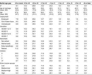
Table A-1: Selected descriptive statistics of the complete pairs subpopulation (n = 4,716)
Marital age gap +8 or more +5 to +8 +2 to +5 +1 to +2 –1 to +1 –1 to –2 –2 to –5 –5 to –8 –8 or less
%* 8.1 12.2 29.6 13.2 23.2 5.3 5.9 1.6 0.9
Age at marriage
(mean, SD) 30.8(8.4) 28.8(8.3) 28.0(7.4) 28.0(6.8) 28.9(6.4) 31.3(7.0) 34.1(7.3) 40.3(8.1) 42.6(5.4) Age
(mean, SD) 47.8(9.7) (10.1)48.4 (10.1)49.0 (10.0)48.5 (10.2)47.5 47.0(9.3) 47.9(9.6) 51.5(7.6) 52.3(7.5) Employment
Employed 7.8 12.0 29.6 12.7 23.7 5.9 5.8 1.6 0.9
Out of labor force 9.3 13.0 28.6 15.2 21.4 3.3 6.3 1.7 1.2
Unemployed 6.8 8.5 39.0 13.6 22.0 5.1 0.0 3.4 1.7
Education
ISCED 1 or 2 9.9 14.2 30.2 13.4 18.1 4.3 6.4 2.0 1.5
ISCED 3 7.5 11.9 26.9 15.7 21.6 6.7 7.5 1.5 0.7
ISCED 5 or 6 7.7 11.4 30.1 13.0 24.4 5.5 5.5 1.6 5.9
ISCED 7 6.6 15.6 19.8 15.1 27.8 6.1 8.0 0.5 0.5
Retirement
Not retired 8.0 12.2 29.6 12.8 23.3 5.7 5.9 1.6 0.9
Retired early 13.6 12.8 27.7 12.8 18.2 2.5 7.0 2.5 2.9
Early beneficiary 4.6 11.7 31.6 18.9 23.8 3.9 4.2 0.7 0.7
Retired 11.5 10.3 26.4 13.8 28.7 2.3 4.6 2.3 0.0
Children
0 19.0 13.8 24.6 11.8 15.9 3.5 8.0 2.1 1.4
1 10.3 13.1 27.8 11.7 19.8 5.0 7.3 3.3 1.9
2 7.0 12.3 30.3 13.3 24.7 5.2 5.1 1.3 0.8
3+ 6.7 11.1 30.0 14.1 23.6 6.3 6.2 1.4 0.6
Gross income spouse
Low 12.6 17.3 31.9 11.6 16.5 3.2 4.6 1.3 0.9
Medium-low 9.3 10.8 30.1 12.6 22.4 5.1 6.8 1.7 1.2
Medium-high 4.8 12.3 29.1 14.4 24.8 7.1 5.4 1.4 0.8
High 6.3 9.1 27.4 14.0 28.1 5.8 6.4 2.1 0.9
Table A-2: Descriptive statistics of the all-twins population (n = 13,354)
Marital age gap +8 or more +5 to +8 +2 to +5 +1 to +2 –1 to +1 –1 to –2 –2 to –5 –5 to –8 –8 or less
%* 9.1 12.7 28.7 13 22.3 5.3 6.3 1.8 0.8
Age at marriage (mean, SD)
30.9 (8.5)
29.3 (8.3)
28 (7.4)
28.5 (7.3)
29.2 (6.9)
31.8 (7.1)
34.9 (7.4)
39.6 (7.8)
43 (5.5) Age
(mean, SD) (10.3)47.2 47.9(10.8) 48.9(10.6) (10.6)48.7 (10.7)47.6 47.7(9.7) 48.5(9.3) 51(8.3) 52.2(7.9) Employment
Employed 9.0 12.4 28.5 12.9 22.9 5.6 6.5 1.7 0.7
Out of labor force 9.6 13.9 29.7 13.4 20.6 4.3 5.8 2.0 0.8
Unemployed 11.6 9.5 27.6 13.1 25.1 4.0 4.0 4.0 1.0
Education
ISCED 1 or 2 11.2 14.3 30.1 12.7 18.1 4.1 6.1 2.3 1.0
ISCED 3 10.8 14.9 25.7 16.5 18.9 4.9 5.9 1.4 1.1
ISCED 5 or 6 8.5 12.0 28.7 13.0 23.6 5.6 6.3 1.6 0.7
ISCED 7 9.2 13.6 23.4 13.4 24.7 6.8 7.5 1.3 0.2
Retirement
Not retired 9.2 12.6 29.3 12.9 22.7 5.5 6.4 1.7 0.7
Retired early 13.4 14.2 29.4 10.8 16.7 3.8 7.6 2.7 1.5
Early beneficiary 5.7 12.6 33.5 15.9 22.2 3.8 4.4 1.4 0.5
Retired 8.8 10.5 27.0 26.9 24.0 5.4 4.1 2.7 0.7
Children
0 19.2 14.5 24.1 9.7 17.0 4.2 7.2 2.4 1.7
1 12.3 12.4 26.7 11.5 21.3 4.6 7.2 2.9 1.1
2 7.8 12.7 29.7 13.5 23.2 5.5 5.8 1.3 0.6
3+ 7.4 12.3 29.3 13.9 22.7 5.5 6.4 1.9 0.7
Gross income spouse
Low 15.0 16.2 30.2 10.6 17.5 3.4 4.5 1.6 0.9
Medium-low 8.8 12.0 29.9 13.1 21.3 5.4 6.8 1.9 0.9
Medium-high 6.2 12.0 28.4 14.7 23.9 6.0 6.6 1.5 0.6
High 6.7 10.6 26.5 13.7 26.5 6.3 7.1 2.1 0.6
Table A-3: Conditional distribution of covariates according to quantiles of the gross income distribution (all percentages)
Completed pairs (n = 4,716) All twins (n = 13,357)
Quantile 0.1 0.25 0.5 0.75 0.9 0.1 0.25 0.5 0.75 0.9
Employment status
Employed 27.6 33.4 83.9 95.4 97.7 24.2 33.1 83.1 94.5 96.8
Out of labor force 71.4 63.0 14.2 4.1 1.9 74.9 62.8 14.8 4.9 2.6
Unemployed 1.0 3.6 2.0 0.5 0.4 0.9 4.1 2.1 0.6 0.5
Education
ISCED 1 or 2 46.4 38.3 23.8 12.7 7.7 46.7 39.7 24.2 14.1 8.9
ISCED 3 2.9 3.3 2.9 2.6 3.2 3.6 2.9 2.8 2.7 2.4
ISCED 5 or 6 49.5 57.3 72.4 82.9 83.0 48.1 56.6 72.0 81.5 81.8
ISCED 7 1.2 1.1 0.9 1.7 6.1 1.6 0.8 1.0 1.7 6.8
Retirement status
Not retired 52.9 53.7 90.4 97.8 99.1 51.5 54.1 90.3 97 98.6
Retired early 30.5 12.1 2.4 0.7 0.3 31.0 12.7 2.9 1.1 0.5
Early beneficiary 8.6 28.8 5.9 1.3 0.5 7.3 28.1 5.7 1.6 0.7
Retired 8.1 5.4 1.4 0.2 0.1 10.2 5.1 1.1 0.3 0.2
Number of children
0 10.5 7.7 4.6 5.5 5.7 10.8 7.9 6.0 6.8 7.3
1 15.2 12.7 15.6 13.5 11.6 15.4 14.1 14.9 14.9 14.0
2 46.0 50.3 51.9 54.2 56.2 45.8 49.4 52.3 52.9 53.3
3+ 28.3 29.3 27.9 26.8 26.5 28.0 28.6 26.8 25.5 25.4
Spouse’s gross income
Low 41.2 41.7 24.3 15.5 12.6 44.0 44.4 23.1 17.3 13.6
Medium-low 21.9 21.5 31.7 30.6 20.5 20.9 22.1 31.5 29.9 22.3
Medium-high 16.7 18.9 24.1 29.4 31.8 15.8 16.9 25.1 29.0 30.9
High 20.2 17.9 20.0 24.5 35.0 19.3 16.6 20.3 23.8 33.3
Supplementary sensitivity analyses – log-income specification and retirement specific models
In our analysis, we have considered as the main outcome the gross income of female twins in 2010. Therefore, the relationship examined by the models presented and discussed in our main analysis can be interpreted (within each quantile) as the absolute increment (or decrement) of the annual gross income per each additional year of age difference relative to the partner.