Depth recovery for unstructured farmland road image using an improved
SIFT algorithm
Lijian Yao
,
Dong Hu
*,
Zidong Yang
,
Haibin Li
,
Mengbo Qian
(School of Engineering, Zhejiang A&F University, Hangzhou 311300, China)Abstract: Road visual navigation relies on accurate road models. This study was aimed at proposing an improved scale-invariant feature transform (SIFT) algorithm for recovering depth information from farmland road images, which would provide a reliable path for visual navigation. The mean image of pixel value in five channels (R, G, B, S and V) were treated as the inspected image and the feature points of the inspected image were extracted by the Canny algorithm, for achieving precise location of the feature points and ensuring the uniformity and density of the feature points. The mean value of the pixels in 5×5 neighborhood around the feature point at an interval of 45º in eight directions was then treated as the feature vector, and the differences of the feature vectors were calculated for preliminary matching of the left and right image feature points. In order to achieve the depth information of farmland road images, the energy method of feature points was used for eliminating the mismatched points. Experiments with a binocular stereo vision system were conducted and the results showed that the matching accuracy and time consuming for depth recovery when using the improved SIFT algorithm were 96.48% and 5.6 s, respectively, with the accuracy for depth recovery of –7.17%-2.97% in a certain sight distance. The mean uniformity, time consuming and matching accuracy for all the 60 images under various climates and road conditions were 50%-70%, 5.0-6.5 s, and higher than 88%, respectively, indicating that performance for achieving the feature points (e.g., uniformity, matching accuracy, and algorithm real-time) of the improved SIFT algorithm were superior to that of conventional SIFT algorithm. This study provides an important reference for navigation technology of agricultural equipment based on machine vision.
Keywords: scale-invariant feature transform (sift), feature matching, canny operator, energy method of feature point, farmland road, depth recovery, visual navigation
DOI: 10.25165/j.ijabe.20191204.4821
Citation: Yao L J, Hu D, Yang Z D, Li H B, Qian M B. Depth recovery for unstructured farmland road image using an improved SIFT algorithm. Int J Agric & Biol Eng, 2019; 12(4): 141–147.
1 Introduction
Intelligent agricultural machinery navigation technology, based on machine vision, has achieved an increasing attention in last decades due to the advantages of rich details of farmland and superior adaptability to complicated environment. Road recognition, coupled with three-dimension (3D) reconstruction is one of the research hotspots. West[1] solved the influence of shadow on image extraction by using color information in road images. Feng et al.[2-4] proposed a method for the determination of appropriate driving paths for navigation vehicle by analyzing the color and gray features in different areas. In order to extract the crop center directly under illumination for driving purposes, Bengochea-Guevara et al.[5] used a threshold segmentation method, considering the field contour and crop type. In the study of Bao et
Received date: 2018-12-04 Accepted date: 2019-06-11
Biographies: Lijian Yao, Associate Professor, research interests: intelligent agricultural equipment and agricultural robot, Email: [email protected]; Zidong Yang, Professor, research interests: design method of modern agricultural equipment, Email: [email protected]; Haibin Li, Assistant Professor, research interests: bionic materials and intelligent algorithms, Email: [email protected]; Mengbo Qian, Associate Professor, research interests: digital innovative design and nonlinear dynamics of mechanisms, Email: [email protected].
*Corresponding author: Dong Hu, PhD, Assistant Professor, research interests: quality and safety detection of agro-products based on light transfer property and spectral imaging, Zhejiang A&F University, 666 Wusu Street, Lin’an District, Hangzhou 311300, China. Tel: +86-15158131053, Email: [email protected].
al.[6], a trapezoid prediction model was first used to detect the edge shape characteristics of the road, and then an improved support vector machine (SVM) classifier was utilized to recognize the road connected area. Choi et al.[7] focused on the study of texture, morphology and other geometric features of the work area to overcome the impact of environmental changes on road images. In addition, neural network has also been introduced into the study of route identification and obstacle location[8,9].
cosine similarity, and achieved the matching success rate of 89.55%. Tian et al.[16,17] adopted multi-thread SIFT feature point detection method for decreasing the time-consuming of road detection successfully. In order to integrate feature matching underwater acoustic image navigation, Li et al.[18] used SIFT feature matching algorithm for extracting feature points of underwater acoustic images. In order to obtain the position error and yaw error simultaneously by the SAR scene matching assistant navigation system, Ren et al.[19] proposed an image matching algorithm based on SIFT.
Previous studies mainly focused on the use of image processing techniques to identify navigation routes, while less attention has been paid to the microscopic details of farmland roads. Although the speeded up robust features (SURF) and SIFT algorithm have been used for feature extraction and matching of the farmland road, the improvement of real-time performance and matching accuracy is in great demand. The SIFT algorithm is advantageous in keeping constant in scene rotation, scale scaling and brightness change. Moreover, the changes of the rotation and scaling between left and right images can be neglected, when the binocular camera is placed in parallel at a small distance, so the redundant information of rotation and scaling can be abandoned to improve the real-time performance of the SIFT algorithm. Therefore, the objective of this study is to improve and optimize the SIFT algorithm for accurate depth recovery of farmland roads under machine vision conditions. The Canny operator was first used to locate the image feature points, considering the density and uniformity of the feature point distribution. Then the feature vectors of feature points in different color spaces were extracted, which were used for matching the left and right image features. Finally, the mismatched pairs were eliminated using the energy method, after which the depth recovery was achieved. The specific objectives were to: (1) optimize the SIFT algorithm by combining the Canny operator; (2) validate the performance of the improved SIFT algorithm using field experiments.
2 Materials and methods
2.1 Materials
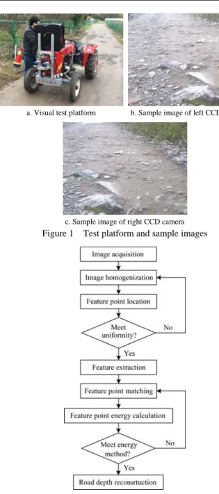
A parallel binocular stereo vision system was used in this study, which mainly consists of a pair of Panasonic CCD cameras (WV-CP480/CH), Seiko lenses (SSV0358), an image acquisition card (DH-CG300) and a computer (Core i5, 3.2GHz, 8G). The visual system was mounted on the front of the tractor (Huanghai Jinma 250B). The images were acquired on the farm track of Guantang experimental farm in Zhejiang A&F University, with the size of 640×480 pixels. The calibration and error correction of the visual system were carried out before image acquisition, and MATLAB 2012b (Mathworks, Inc., Natick, Massachusetts, USA) was used to analyze the images. The platform and acquired images of the left and right cameras are shown in Figures 1a, 1b and 1c, respectively.
2.2 Image processing
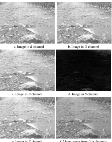
The flowchart of image processing in this study is shown in Figure 2. The acquired image was first subjected to homogenization processing and feature point location, and then it was judged whether the uniformity of the image met the requirement. If the requirement was met, image feature extraction, feature point matching, and feature point energy calculation were sequentially performed, otherwise it returned to the homogenization process. The images, which met the requirement of energy method, were finally used for depth recovery.
a. Visual test platform b. Sample image of left CCD camera
c. Sample image of right CCD camera Figure 1 Test platform and sample images
Figure 2 Flowchart for image processing 2.2.1 Preprocessing of inspected image
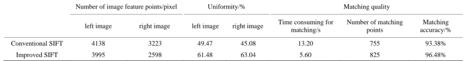
The conventional SIFT algorithm extracts the feature points in the positions where the pixel values of the image change sharply, but it pays little attention to the uniformity of the feature point distribution. Some researchers proposed a feature point extraction method based on region segmentation to ensure the uniformity of feature point distribution[20,21], but the algorithm was not well in real-time. RGB and HSV are two common color spaces, and the positions with the pixel values changing sharply are different, resulting in inconsistent distribution uniformity of the extracted feature points. In order to improve the distribution uniformity of the feature points, three single channel data matrices of R, G and B, coupled with the saturation S and the gray level V data matrix in the HSV space, were used in this study. The new inspected image matrix Imean, which was the mean image of pixel value in five channels, could be calculated as follows:
Imean=(IR+IG+IB+IS+IV)/5 (1) where, IR, IG, IB, IS and IV are the pixel values of the road image in
a. Image in R-channel b. Image in G-channel
c. Image in B-channel d. Image in S-channel
e. Image in V-channel f. Mean image from five channels Figure 3 Images for different channels
2.2.2 Extracting feature points
The Canny operator is a multi-level edge detection algorithm[22], which could suppresses noise effectively and determines edge position accurately. In this study, preliminary extraction and positioning for the feature points of the new inspected image were firstly conducted by the Canny operator. Then eigenvalue of the feature points was determined by using the SIFT algorithm. Discrete Gaussian Filter in the Canny operator, taking care of both the main outlines and tiny details of the image, could further improve the uniformity of the feature point distribution. Figure 4a was a binary image for the feature point distribution extracted by the above method. To better express the specific location of these feature points, the feature points were enlarged and displayed in a true color scene image, as shown in Figure 4b. The Canny operator used in this study had a 2D discrete Gaussian 9×9 filter with the standard deviation as 1 and the ratio of low threshold to high threshold as 0.4, resulting in the number of feature points as 3995.
a. Binary map b. Feature point distribution in true color scene
Figure 4 Distribution of feature points 2.2.3 Quantitative analysis of feature point uniformity
Assuming that the number of feature points extracted by the method in Section 2.2 is T. In order to quantitatively analyze its uniformity, the image in Figure 4a was evenly divided into k block regions. Here it was divided into 25 pieces (5×5), with the size of
128×96 pixels for each piece. The uniformity of the feature point distribution was described using a variable U, which could be calculated using Equation (2).
1
1 [ ( / ) ] / ( ) 100%
k
i i
U N T k k T
=
⎧ ⎫
=⎨ − − ⋅ ⎬×
⎩
∑
⎭ (2)where, Ni was the number of feature points of block i, and T was the total number of the feature points.
Since the Equation (2) has been normalized, the closer U value is to 1, the better the uniformity of feature points is. Therefore, the feature point uniformity of the conventional SIFT method and the method proposed in this study can be compared using the value of U. In a picture of the same size, the larger the number of feature points, the higher the density. To ensure that the uniformity of the feature point distribution of the two methods was compared under the same density, a specific threshold was set in the SFIT algorithm to make the number of feature points basically equal[8].
Figures 5a and 5b showed the feature point distribution extracted by the conventional SIFT method and the proposed method under a single channel (R channel), respectively. Table 1 was the corresponding quantitative analysis for the feature point uniformity. It was observed that the feature point uniformity extracted by the method proposed in this study was better than the conventional SIFT algorithm. Moreover, the performance of the mean operation for multi-channel images was superior to that with only a single channel.
a. Conventional SIFT method b. Proposed method in R-channel Figure 5 Distribution of feature points using different methods
Table 1 Quantitative analysis for the feature point uniformity
Conventional SIFT Proposed method for R-channel
Proposed method for five channels Number of image
feature points/pixel 4138 3935 3995
Uniformity/% 49.47% 39.57% 61.48%
2.2.4 Extracting feature value
Feature value is important to serve as the matching basis for depth reconstruction of the farmland road images. The feature vectors extracted by the conventional SIFT algorithm had the characteristics of invariance to scene rotation and scaling. The rotation and scaling changes of the left and right images were negligible when the binocular camera was placed parallel to each other at a small distance. However, the affine transformation between the left and right images could not be ignored due to the parallax between the left and right cameras. In order to improve the real-time performance of the algorithm, the redundant information, such as rotation and scale scaling, was abandoned. Since the feature points of the image were obtained based on the mean values of R, G, B, S and V, the feature values were also extracted in the five channels to describe the feature points. The specific steps were as follows:
necessary to investigate the information of other points adjacent to this feature point. The neighborhood scope was increased in this study to lower the effect of the affine transformation between images. Therefore, for a feature point f(x,y) in a channel, the pixel values in the neighborhood of 5×5 were analyzed (Figure 6a). The values of v(1)-v(8) in eight directions around the feature point
f(x,y) at an interval of 45 degrees were used to represent the feature vector of this point, as shown in Figure 6b. The values of v(1)-v(8) can be calculated using Equation (3):
(1) [ ( 2, 2) ( 1, 2) ( 2, 1) ( 1, 1)] / 4 (2) [ ( 1, 2) ( , 2) ( 1, 2) ( 1, 1) ( , 1)
( 1, 1))] / 6
v = f x- +f x- +f x- +f x-
y-v = f x- y- +f x y- +f x+ y- +f x- y- +f x y- + f x+
y-⎧ ⎪ ⎪ ⎨ ⎪ ⎪⋅⋅⋅⋅⋅⋅ ⎩
(3) where, v(1) and v(2) were the mean values of the pixels in the corresponding red and blue dotted box in Figure 6a, respectively. In this way, a 5×8 feature vector V was generated for each feature point. The feature vector V was able to restrain image noise and maintain the stability for the affine transformation, since it was calculated as the mean value.
a. 5×5 neighborhood of a feature point
b. Feature vectors for each channel Figure 6 Extraction of feature value
Step2: Determine the initial matching point pair. The Marr Polar Constraint principle was used to narrow the range of potential matching point pairs of left and right images, followed with Equation (4) for calculating the difference between the feature values of point pairs. Assuming that the 5×8 feature vectors of a feature point in the left and right images were VL and VH, respectively, DL-H was used to describe the difference between the two feature points:
5 8
L H
L-H
1 1
( ) ( )
i i
i j
D = V j V j
= =
−
∑∑
(4)The smaller value of DL-H indicates the smaller difference between the two feature points. Hence the point pair with the
minimum DL-H value was the initial matching point pair.
Step3: Eliminate the mismatching point. Although the information of the neighborhood of the point was fully utilized in searching for the initial matching point pair, there still remained mismatching points. Fox example, the point in Figure 7a indicated by the arrow matched the point indicated by the arrow in Figure 7b according to the Equation (4), but obviously they did not match. The correct matching point should be the point indicated by the arrow in Figure 7c.
a. Matching point of left image b. Error matching point of right image
c. Correct matching point of right image Figure 7 Elimination of the error matching point
The mismatching points were eliminated by calculating the energy of feature points in this study[23]. This method made full use of the relationship between the current initial matching point and the surrounding matching point, with the main idea as follows: 1) Determine the initial matching point pairs fl(x,y) and fr(x,y); 2) Determine the initial matching point collections Ml and Mr, which were centered on the left and right points, respectively, with the parameter φ as the radius. The more the number of initial matching point pairs in the collection, the greater the energy of the feature point. PL-H was used to describe the probability of correct matching point pair, which could be calculated using Equation (5):
-L-H
( ) / 2
l r
l r
m P
m m
=
+ (5)
where, ml and mr were the element number in the two collections, which were also called energy, and ml-r was the number of successful initial matching point pairs in the two collections. The larger the PL-H was, the greater probability that the point pairs matched correctly.
The appropriate threshold value P was then used to judge whether the initial matching point was the correct matching point. According to the coordinate information of the correct matching point pair, the depth information Z of each matching point in the farmland road could be calculated by Equation (6):
2 | r l|
af Z
x x
=
− (6)
3 Results and discussion
60 pairs of farmland road images were acquired using the above calibrated test platform for validating the effectiveness of the proposed algorithm in this study. The images were acquired in different conditions, such as sunny, partly cloudy and cloudy for the weather conditions, and straight road, curve road, upper and lower ramp road, and watery road for the road conditions. Figure 8 shows part of farmland road images acquired in different conditions. Depth information measurement was conducted on the test sites, which was further used to compare with the experimental results for validating the performance of the proposed
method in this study. Figure 9(a) was the sample image of the left CCD camera in Figure 1, in which ten artificial measurement points of depth information were labeled, and Figures 9b and 9c were the contour map of depth information and 3D depth map after 3D depth reconstruction, respectively. The projection size was the same as the sample image. The value of a certain point in Figures 9b and 9c was the distance between the corresponding point in the road surface and the center point of the binocular camera. Table 2 and Table 3 were summaries for the matching quality of the left and right image in Figure 1, and error statistics of depth information recovery, respectively.
a. Curve/Partly Cloudy b. Ramp/Sunny c. Watery/Cloudy d. Straight/Cloudy
Figure 8 Farmland road images in different conditions
a. Schematic diagram of test point positions b. Contour map of depth information c. 3D depth map Figure 9 Depth information retrieval for farmland road
Table 2 Comparison of matching quality for left and right images
Table 3 Error statistics of depth information recovery for farmland road
Point 1 Point 2 Point 3 Point 4 Point 5 Point 6 Point 7 Point 8 Point 9 Point 10 Measured value/m 2.51 1.91 1.61 1.38 1.34 1.30 1.21 0.96 1.01 1.00
Test values/m 2.33 1.80 1.53 1.32 1.29 1.25 1.19 0.98 1.04 1.01
Error/% –7.17% –5.76% –4.97% –4.35% –3.73% –3.85% –1.65% 2.08% 2.97% 1.00%
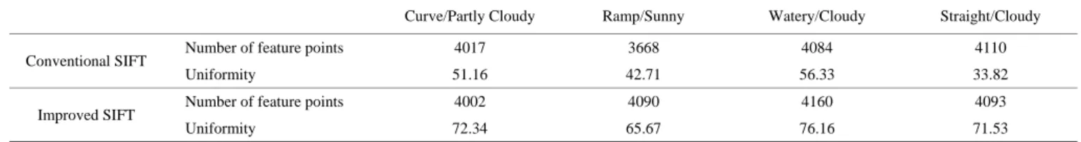
In order to test the versatility of the proposed algorithm, feature point matching and depth recovery experiments were conducted for 60 pairs of farmland road images. Figure 10 was comparison of the feature point distribution extracted by the conventional and improved SIFT algorithms from part of the images in Figure 8. Table 4 shows statistical results for the number and uniformity of the feature points, and Table 5 shows the comprehensive statistics for the matching quality of these 60 pairs of images by using the improved SIFT algorithm.
The following conclusions can be drawn from the experimental analysis:
(1) It was observed from Table 2 that the successful matching
point pairs by the conventional and improved SIFT algorithms were 755 and 825, respectively, and the utilization ratio for the feature points were 20.51% and 25.03%, indicating that the proposed method in this study had higher utilization efficiency for the obtained feature points. Though both the two methods had relatively high matching accuracy, time consuming of the proposed method was 5.60 s, approximately two fifths of the conventional SIFT algorithm, which significantly improved the real-time performance for the feature point matching.
(2) As shown in Figure 9 and Table 3, the depth reconstruction accuracy using the calibrated binocular stereo vision system was within –7.17%-2.97%. The camera had smaller distortion when Number of image feature points/pixel Uniformity/% Matching quality
left image right image left image right image Time consuming for matching/s
Number of matching points
Matching accuracy/%
Conventional SIFT 4138 3223 49.47 45.08 13.20 755 93.38%
the farmland road was closer to the camera, resulting in smaller error, and the accuracy could be ±5% when the depth was within 2 m. These results showed that the method proposed in this study
could accurately restore the 3D landform of farmland road, which provided a fundamental basis for visual navigation and vehicle control.
a1 a2 a3 a4
b1 b2 b3 b4 Figure 10 Comparison of the feature point distribution for part of images extracted by the conventional (top panel) and improved (bottom
panel) SIFT algorithms, where the images from left to right were curve/partly cloudy, ramp/sunny, watery/cloudy, and straight/cloudy, respectively
Table 4 Statistics of the number and uniformity of the feature points for part of images extracted by the conventional and improved SIFT algorithms
Curve/Partly Cloudy Ramp/Sunny Watery/Cloudy Straight/Cloudy
Conventional SIFT Number of feature points 4017 3668 4084 4110
Uniformity 51.16 42.71 56.33 33.82
Improved SIFT Number of feature points 4002 4090 4160 4093
Uniformity 72.34 65.67 76.16 71.53
Table 5 Statistics of matching quality for 60 groups of images by the improved SIFT algorithm.
Road conditions Climate conditions
Straight (30 pictures)
Curve (18 pictures)
Ramp (12 pictures)
Sunny (20 pictures)
Partly Cloudy (20 pictures)
Cloudy (20 pictures)
Average uniformity/% 62.85 59.70 56.54 65.12 61.28 52.68
Average time/s 6.05 5.45 5.70 6.25 5.75 5.2
Average matching accuracy/% 95.45 93.04 90.84 96.21 94.73 88.4
(3) As shown in Figure 10 and Table 4, the uniformities of feature point distribution by using the conventional and improved SIFT algorithms were 33.82%-56.33% and 65.67%-76.16%, in the case where the density of feature points was basically the same (around 4000 pixels), indicating that the method proposed in this study performed much better. Moreover, the uniformity for the conventional SIFT algorithm was only 33.82% when the road condition was relatively straight (Figure 10a4), which was much worse than that obtained by the improved SIFT algorithm (71.53%).
(4) It was observed from Table 5 that the mean uniformity, time consuming, and matching accuracy for feature points by the improved SIFT algorithm were 50%-70%, 6-6.5 s, and higher than 88%, respectively. Different road conditions and weather conditions have great influence on the matching quality. Straight road and sunny weather performed better matching quality. However, bad weather increased the difficulty in acquiring high quality images, and the curve or ramp road caused a large difference in road features between the left and right images, with
some of the feature points located in the region with large camera distortion, thus reducing the overall matching accuracy.
4 Conclusions
both the matching quality and depth recovery accuracy should be improved in bad conditions, such as cloudy weather and ramp road. Moreover, the accuracy of the road model should be verified by laser scanning technology to make the farmland road model closer to the real road surface.
Acknowledgements
This work was financially supported by the Zhejiang Science and Technology Department Basic Public Welfare Research Project (LGN18F030001) and the Major Project of Zhejiang Science and Technology Department (2016C02G2100540).
[References]
[1] West B. Enhanced visual navigation for mobile robots. Auburn: Auburn University, Alabama,USA, 2014.
[2] Feng J, Liu G, Si Y. Algorithm based on image processing technology to generate navigation directrix in orchard. Transactions of the CSAM, 2012; 43(7): 185–189, 184. (in Chinese).
[3] Li J, Chen B, Liu Y. Detection for navigation route for cotton harvester based on machine vision. Transactions of the CSAE, 2013; 29(11): 11–19. (in Chinese).
[4] Li Y, Wei L. Navigation line of vision extraction algorithm based on dark channel. Acta Optica Sinica, 2015; 35(2): 0215001. (in Chinese). [5] Bengochea-Guevara J M, Conesa-Muñoz J, Andújar D, Ribeiro A. Merge
fuzzy visual servoing and GPS-based planning to obtain a proper navigation behavior for a small crop-inspection robot. Sensors, 2016; 16: 276.
[6] Bao J, Zhang Y, Su X, Zheng R. Unpaved road detection based on spatial fuzzy clustering algorithm. EURASIP Journal on Image and Video Processing, 2018; 2018: 26.
[7] Choi K H, Han S K, Han S H, Park K H, Kim K S, Kim S. Morphology-based guidance line extraction for an autonomous weeding robot in paddy fields. Computers and Electronics in Agriculture, 2015; 113: 266–274.
[8] Cong Y, Peng J J, Sun J, Zhu L L, Tang Y D. V-disparity based UGV obstacle detection in rough outdoor terrain. Acta Automatica Sinica, 2010; 36: 667–673.
[9] Tang J, Jing X, He D. Visual navigation control for agricultural robot
using serial BP neural network. Transactions of the CSAE, 2011; 27(2): 194–198.
[10] Kostavelis I, Boukas E, Nalpantidis L, Gasteratos A. Stereo-based visual odometry for autonomous robot navigation. International Journal of Advanced Robotic Systems, 2016; 13: 21.
[11] Vitor G B, Victorino A C, Ferreira J V. Comprehensive performance analysis of road detection algorithms using the common urban Kitti-road benchmark. Intelligent Vehicles Symposium Proceedings, 2014; pp.19–24. [12] Li Y, Olson E B. A general purpose feature extractor for light detection
and ranging data. Sensors, 2010; 10: 10356–10375.
[13] Lowe D G. Distinctive image features from scale-invariant keypoints. International Journal of Computer Vision, 2004; 60: 91–110.
[14] Shao N, Li H G, Liu L, Zhang Z L. Stereo vision robot obstacle detection based on the SIFT. 2010 Second WRI Global Congress on Intelligent Systems, 2010; pp.274–277.
[15] Guo A, Xiong J, Xiao D. Computation of picking point of litchi and its binocular stereo matching based on combined algorithms of harris and SIFT. Transactions of the CSAM, 2015; 46(12): 11–17. (in Chinese) [16] Li S, Zhou J, Ji C, Tian G, Gu B, Wang H. Moving obstacle detection
based on panoramic vision for intelligent agricultural vehicle. Transactions of the CSAM, 2013; 12: 041. (in Chinese)
[17] Tian G, An Q, Ji C. Real-time motion detection for intelligent agricultural vehicle based on stereo vision. Transactions of the CSAM, 2013; 44(7): 210–215. (in Chinese).
[18] Li K, Zhang L. Research on underwater navigation algorithm based on SIFT matching algorithm. DEStech Transactions on Engineering and Technology Research, 2017.
[19] Ren S, Chang W, Liu X. SAR image matching method based on improved SIFT for navigation system. Progress in Electromagnetics Research, 2011; 18: 259–269.
[20] Ni X, Ding L, Jiang T, Hu S. A remote sensing image registration algorithm by obtaining uniform control points based on invariant feature. Science of Surveying and Mapping, 2011; 36: 70–72.
[21] Wu C, Niu H, Liang W. A new homogenized feature based multi-spectral image registration method. 2012 Third Global Congress on Intelligent Systems, 2012; pp.198–201.
[22] Schalkoff R J. Digital image processing and computer vision. Wiley New York, 1989.