ISSN: 2231-5373
http://www.ijmttjournal.org
Page 437
Efficient Hierarchic Predictive Multivariate
Product Estimator Based On Harmonic Mean
K.B.Panda1 and P.Das2
Department of Statistics, Utkal University, Bhubaneswar, Odisha, India
Abstract−In this paper, extending the work of hierarchic estimation proposed by Agrawal and Sthapit(1997), we define a multivariate product estimator using harmonic means of multi-auxiliary variables which conforms to predictive character. Furthermore, it has been shown that the proposed multivariate product estimator of order k, when k is determined optimally, fares better than its competitors both in terms of bias and mean square error under some practical conditions. Empirical investigations in support of the theoretical findings have been carried out.
Keywords−Hierarchic multivariate product estimator, auxiliary information, harmonic mean
I. INTRODUCTION
In the literature of survey sampling, the use of auxiliary information at estimation stage often results in considerable gain in efficiency of the proposed estimators for population parameters under study. Singh(1967) has utilized multi-auxiliary variables negatively correlated with the study variable to propose the customary multivariate product estimator. Adhering to the method of hierarchic estimation introduced by Agrawal and Sthapit(1997) and carried forward by Panda and Sahoo(2015), this paper develops a new multivariate product estimator of order k using harmonic means of multi-auxiliary variables.
Let 𝑈 = 𝑈1, 𝑈2, … … … . , 𝑈𝑁 be the finite population of size 𝑁, out of which a sample of size𝑛 is drawn with simple random sampling without replacement. Let 𝑦 and 𝑥𝑖(𝑖 = 1,2, … … , 𝑝) be, respectively, the study and 𝑖-th auxiliary variables having population means 𝑌 and 𝑋 𝑖 (known), and sample means 𝑦 and 𝑥 𝑖 . The auxiliary variable 𝑥𝑖(𝑖 = 1,2, … … , 𝑝) is assumed to be negatively correlated with the study variable 𝑦. Let 𝜌𝑜𝑖 and 𝜌𝑖𝑗, respectively, denote the correlation coefficients between 𝑦 and 𝑥𝑖 and 𝑥𝑖 and 𝑥𝑗 𝑖 ≠ 𝑗 = 1, … … , 𝑝 and 𝐶0 and
𝐶𝑖(𝑖 = 1, … … , 𝑝) be, respectively, the coefficients of variation of 𝑦 and 𝑥𝑖. Let’s further suppose that 𝐶0𝑖 =
𝜌0𝑖𝐶0𝐶𝑖 and 𝐶𝑖𝑗 = 𝜌𝑖𝑗𝐶𝑖𝐶𝑗 .
The traditional multivariate product estimator due to Agrawal and Panda (1993) is given by
𝑦 𝑀𝑃𝐻 = 𝑦 𝑝𝑖=1𝑤𝑖𝑥 𝑖,/𝑋 𝑖 , (1.1)
where𝑤𝑖′𝑠 are weights such that 𝑝𝑖=1𝑤𝑖 = 1, its bias and mean square error , to the first degree of approximation, i.e., to 𝑜(𝑛−1) have been expressed, respectively, as
𝐵 𝑦 𝑀𝑃𝐻 = 𝜃𝑌 𝑝𝑖=1𝑤𝑖𝐶𝑖2+ 𝑝𝑖=1𝑤𝑖𝐶0𝑖 (1.2) and𝑀 𝑦 𝑀𝑃𝐻 = 𝜃𝑌 2 𝐶02+ 𝑃𝑖=1𝑤𝑖2𝐶𝑖2+ 𝑃𝑖≠𝑗𝑤𝑖𝑤𝑗𝐶𝑖𝑗 + 2 𝑃𝑖=1𝑤𝑖𝐶0𝑖 (1.3)
= 𝒘𝑩𝒘𝑇,
where𝒘 = (𝑤1, 𝑤2, … … … , 𝑤𝑝) is a p-vector, 𝑩 = (𝑏𝑖𝑗), 𝑏𝑖𝑗 = 𝜃𝑌 2 𝐶02+ 𝐶0𝑖+ 𝐶0𝑗+ 𝐶𝑖𝑗 (i≠ 𝑗 = 1, … . . , 𝑝) and 𝜃 =1𝑛−𝑁1 . The superscript T refers to transpose. Minimization of the mean square error of𝑦 𝑀𝑃𝐻 yields the following optimal weight vector :
ISSN: 2231-5373
http://www.ijmttjournal.org
Page 438
where𝒆 = 1, 1, … … , 1 and 𝑾 = (𝑊1, 𝑊2, … … … , 𝑊𝑝) are p-vectors. In what follows, we shall consider multivariate product estimator 𝑦 𝑀𝑃 using optimum weights.
Comparing the minimum MSE of𝑦 𝑀𝑃𝐻 given in (1.1) with the variance of simple mean 𝑦 , we find that 𝑦 𝑀𝑃𝐻 fares better than 𝑦 if condition
1 2≤
− 𝑝𝑖=1𝑊𝑖𝐶0𝑖 𝑊𝑖2
𝑝
𝑖=1 𝐶𝑖2+ 𝑝𝑖≠𝑗 =1𝑊𝑖𝑊𝑗𝐶𝑖𝑗 (1.5) holds.
II. THE NEWLY PROPOSED MULTIVARIATE PRODUCT ESTIMATOR
Following the predictive approach of Basu(1971) and Smith(1976), we write the population total as
Y= 𝑦𝑙𝜖𝑠 𝑙+ 𝑦𝑙𝜖 𝑠 𝑙 , (2.1) where𝑠 is the sample of selected units and 𝑠 is its complement. Thus, the first part on the right-hand side of equation (2.1) is known and to estimate Y, we have to predict the second part on the right- hand side of the equation . As a matter of fact, the predictive format for estimation of Y becomes
𝑌 = 𝑦𝑙𝜖𝑠 𝑙+ 𝑦 𝑙𝜖 𝑠 𝑙 , (2.2)
where𝑦 𝑙 is the implied predictor of 𝑦𝑙(𝑙 ∈ 𝑠 ). If we use the multivariate product estimator due to Agrawal and Panda(1993) given in (1.1) as an intuitive predictor of 𝑦𝑙(𝑙 ∈ 𝑠 ), then we arrive at
𝑌 = 𝑦𝑙𝜖𝑠 𝑙 + (N−𝑛) 𝑦 𝑀𝑃𝐻 or𝑌 = 𝑦 𝑀𝑃𝐻(1) , (2.3) where𝑦 𝑀𝑃𝐻(1) = 𝜙1𝑧 𝑀𝑃𝐻 + 𝑦 𝑀𝑃𝐻 , with 𝜙1= 1 +𝜆𝜙0 , 𝜙0= 0, 𝜆 = 1−𝑁𝑛 and𝑧 𝑀𝑃𝐻 = 𝑁𝑛𝑦 1 − 𝑃𝑖=1𝑤𝑖𝑋 𝑥 𝑖
𝑖 .
Now, making use of 𝑦 𝑀𝑃𝐻(1) as an intuitive predictor of 𝑦𝑙(𝑙 ∈ 𝑠 ) in (2.2), we obtain
𝑌 = 𝑦 𝑀𝑃𝐻 2 ,
where𝑦 𝑀𝑃𝐻 2 = 𝜙2𝑧 𝑀𝑃𝐻 + 𝑦 𝑀𝑃𝐻 and 𝜙2= 1+ 𝜆𝜙1. Proceeding in this manner, we would, at the 𝑘𝑡ℎ iteration, reach
𝑦 𝑀𝑃𝐻 𝑘 = 𝜙𝑘𝑧 𝑀𝑃𝐻 + 𝑦 𝑀𝑃𝐻 , where𝜙𝑘= 1 + 𝜆𝜙𝑘−1=1− 𝜆
𝑘
1− 𝜆.
With 𝜙𝑘 as stated above, 𝑦 𝑀𝑃𝐻 𝑘 can be rewritten as
𝑦 𝑀𝑃𝐻 𝑘 = 1 − 𝜆𝑘 𝑦 + 𝜆𝑘𝑦 𝑀𝑃𝐻 (2.4)
We have, thus, arrived at the newly proposed multivariate product estimator of order 𝑘. It is worth mentioning that when 𝑘 = 0, the proposed estimator is same as the customary multivariate product estimator 𝑦 𝑀𝑃𝐻&when
𝑘 → ∞, this becomes 𝑦 . It is apt to mention here that sampling is carried out from a finite population, i.e., when 𝑁 < ∞ , for if we draw samples of fixed sizes from an infinite population, then the proposed estimator
ISSN: 2231-5373
http://www.ijmttjournal.org
Page 439
1 − 𝜆𝑘 𝑦 + 𝜆𝑘 𝑊 𝑖
𝑦 𝑥𝑖𝑗𝑥 𝑖 𝑝
𝑖=1
as the intuitive predictor of 𝑦𝑙(𝑙 ∈ 𝑠 ) in (2.2) and can easily conclude that
𝑌 = 𝑦 𝑀𝑃𝐻 𝑘 ,
which shows that the proposed multivariate product estimator of order 𝑘 (𝑘 ≥ 1) is endowed with the predictive character.
III. COMPARISON OF BIAS AND MEAN SQUARE ERROR OF THE PROPOSED ESTIMATOR VIS-À-VIS THE COMPETING ESTIMATOR
The bias of the estimator 𝑦 𝑀𝑃𝐻 𝑘 , to 𝑜 𝑛−1 , can be found as
𝐵(𝑦 𝑀𝑃𝐻 𝑘 )= 𝜆𝑘𝜃𝑌 𝑖=1𝑝 𝑤𝑖𝐶𝑖2+ 𝑝𝑖=1𝑊𝑖𝐶0𝑖 . (3.1)
It is evident from (3.1) that the absolute value of the bias obtained above is, for 𝑘 ≥ 1, invariably less than that of the customary multivariate product estimator given in (1.2).
The mean square error of 𝑦 𝑀𝑃𝐻 𝑘 ,to 𝑜 𝑛−1 , can be worked out as
𝑀 𝑦 𝑀𝑃𝐻 𝑘 = 𝜃𝑌 2 𝐶02+ 𝜆2𝑘 𝑃𝑖=1𝑊𝑖2𝐶𝑖2+ 𝜆2𝑘 𝑃𝑖≠𝑗 =1𝑊𝑖𝑊𝑗𝐶𝑖𝑗+ 2𝜆𝑘 𝑃𝑖=1𝑊𝑖𝐶0𝑖 (3.2)
= 𝑾𝑩𝑾𝑇, where𝑾 is the p-vector as defined in the foregoing section, 𝐵 = (𝑏𝑖𝑗) and
𝑏𝑖𝑗 = 𝜃𝑌 2 𝐶02+ 𝜆𝑘𝐶0𝑖+ 𝜆𝑘𝐶0𝑗 + 𝜆2𝑘𝐶𝑖𝑗 . When k is determined optimally in order to minimize (3.2) , we get
𝜆𝑘= − 𝑝𝑖=1𝑤𝑖𝐶0𝑖
𝑊𝑖2
𝑝
𝑖=1 𝐶𝑖2+ 𝑝𝑖≠𝑗 =1𝑊𝑖𝑊𝑗𝐶𝑖𝑗. (3.3)
Comparing the minimum mean square error of the multivariate product estimator 𝑦 𝑀𝑃𝐻(using optimum weights in (1.3)) with the mean square error of the proposed multivariate product estimator 𝑦 𝑀𝑃𝐻 𝑘 , we find that the estimator 𝑦 𝑀𝑃𝐻 𝑘 fares better than the estimator 𝑦 𝑀𝑃𝐻 if
1 2(1 + 𝜆
𝑘) ≥ − 𝑝𝑖=1𝑊𝑖𝐶0𝑖
𝑊𝑖2𝐶𝑖2+ 𝑝𝑖≠𝑗 =1𝑊𝑖𝑊𝑗𝐶𝑖𝑗
𝑝
𝑖=1 , (3.4)
and it fares better than 𝑦 if 1 2𝜆
𝑘 ≤ − 𝑝𝑖=1𝑊𝑖𝐶0𝑖
𝑊𝑖2𝐶𝑖2+ 𝑝𝑖≠𝑗 =1𝑊𝑖𝑊𝑗𝐶𝑖𝑗
𝑝
𝑖=1 . (3.5)
Thus, 𝑦 𝑀𝑃𝐻 𝑘 will perform better than both 𝑦 𝑀𝑃𝐻 and 𝑦 when 1
2𝜆
𝑘 ≤ − 𝑝𝑖=1𝑊𝑖𝐶0𝑖
𝑊𝑖2𝐶
𝑖2+ 𝑝𝑖≠𝑗 =1𝑊𝑖𝑊𝑗𝐶𝑖𝑗 𝑝
𝑖=1 ≤
1 2 1 + 𝜆
𝑘 , (3.6)
ISSN: 2231-5373
http://www.ijmttjournal.org
Page 440
1 2𝜆
𝑘 ≤ 𝜆𝑘≤1 2 1 + 𝜆
𝑘 , (3.7)
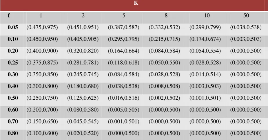
which is invariably true as 𝜆 < 1 and 𝑘 ≥ 1, revealing the supremacy of the proposed estimator over its competitors. The bounds given in (3.6) are called the efficiency bounds, the term in the middle of (3.6) being treated as a pivotal quantity. By choosing values of the sampling fraction 𝑓(=𝑁𝑛) and hence 𝜆(= 1 − 𝑓), we have computed the following table which gives the bounds of − WiC0i
p i=1
Wi2Ci2+ pi≠j=1WiWjCij p
i=1 within which y MPH
k ( for
various values of 𝑘) will be more efficient than 𝑦 𝑀𝑃𝐻 and 𝑦 .
Table 1: Efficiency bounds of − 𝑊𝑖𝐶0𝑖
𝑝 𝑖=1
𝑊𝑖2𝐶𝑖2+ 𝑝𝑖≠𝑗 =1𝑊𝑖𝑊𝑗𝐶𝑖𝑗
𝑝
𝑖=1 for various values of 𝑓 and 𝑘
K
f 1 2 5 8 10 50
0.05 (0.475,0.975) (0.451,0.951) (0.387,0.587) (0.332,0.532) (0.299,0.799) (0.038,0.538)
0.10 (0.450,0.950) (0.405,0.905) (0.295,0.795) (0.215,0.715) (0.174,0.674) (0.003,0.503)
0.20 (0.400,0.900) (0.320,0.820) (0.164,0.664) (0.084,0.584) (0.054,0.554) (0.000,0.500)
0.25 (0.375,0.875) (0.281,0.781) (0.118,0.618) (0.050,0.550) (0.028,0.528) (0.000,0.500)
0.30 (0.350,0.850) (0.245,0.745) (0.084,0.584) (0.028,0.528) (0.014,0.514) (0.000,0.500)
0.40 (0.300,0.800) (0.180,0.680) (0.038,0.538) (0.008,0.508) (0.003,0.503) (0.000,0.500)
0.50 (0.250,0.750) (0.125,0.625) (0.016,0.516) (0.002,0.502) (0.001,0.501) (0.000,0.500)
0.60 (0.200,0.700) (0.080,0.580) (0.005,0.505) (0.000,0.500) (0.000,0.500) (0.000,0.500)
0.70 (0.150,0.650) (0.045,0.545) (0.001,0.501) (0.000,0.500) (0.000,0.500) (0.000,0.500)
0.80 (0.100,0.600) (0.020,0.520) (0.000,0.500) (0.000,0.500) (0.000,0.500) (0.000,0.500)
Table 1 can serve as an aid to locate a suitable value of 𝑘 for given values of the pivotal quantityand 𝑓. Knowledge of the pivotal quantity consisting of various population parameters such as the population correlation coefficients and coefficients of variation, as they remain stable over a period of time, can be gathered from past survey, pilot survey, educated guess etc. For a specified value of the pivotal quantity, Table 1 provides more than one value of 𝑘 which ensures better performance of 𝑦 𝑀𝑃𝐻 𝑘 vis-à-vis 𝑦 𝑀𝑃𝐻 and 𝑦 . However the optimal value of 𝑘 can be arrived at from equation (3.3) provided − 𝑊𝑖𝐶0𝑖
𝑝 𝑖=1
𝑊𝑖2
𝑝
𝑖=1 𝐶𝑖2+ 𝑝𝑖≠𝑗 =1𝑊𝑖𝑊𝑗𝐶𝑖𝑗 < 1. When an optimum
value of 𝑘 is not obtainable, a suitable value of 𝑘 that renders 𝑦 𝑀𝑃𝐻 𝑘 superior to 𝑦 𝑀𝑃𝐻 and 𝑦 might still be found from the above table.
Here attention is drawn to the fact that if any one of the p-weights becomes 1 and the rest are zero each, then the proposed estimator of order 𝑘 will be no different from the one due to Agrawal and Panda(1993) and its mean square error, under optimality of 𝑘, remains same as that of the linear regression estimator.
IV. EMPIRICAL INVESTIGATIONS
For the purpose of empirical investigation, we have considered two auxiliary variables 𝑋1 and 𝑋2 each being negatively correlated with the study variable𝑌.
ISSN: 2231-5373
http://www.ijmttjournal.org
Page 441
We have computed the following population quantities from the information given in Weisberg(1980, p.179), wherein accident rates per million vehicle miles is considered as the study variable 𝑌 which is negatively correlated with the speed limit 𝑋1 and the federal and interstate highway 𝑋2 . Here
𝑋1 and 𝑋2 are being considered as the auxiliary variables:
N=39 and 𝐶𝑖𝑗 =
0.2616 −0.0892 −0.2730 −0.0892 0.2003 0.4779
−0.2730 0.4779 7.1768 (𝑖, 𝑗 = 0, 1, 2)
Making use of these quantities, we have found the optimum weights 𝑊1 , 𝑊2 and the pivotal quantity given in (3.6) as 1.0146, -0.0146 and 0.4493, respectively. For assessing the performance of the proposed estimator 𝑦 𝑀𝑃𝐻 𝑘 over 𝑦 𝑀𝑃𝐻 and 𝑦 , we have prepared the following table:
Table 1: Bias and Mean Square error of Competing Estimators
Estimator Bias/ 𝜃𝑌 MSE/ 𝜃𝑌 2
𝑦 0.0000 0.2616
𝑦 𝑀𝑃𝐻 0.0119 0.2809
𝑦 𝑀𝑃𝐻 𝑘 0.0054 0.2227
From the above table, it is observed thatgain in efficiency of the proposed estimator 𝑦 𝑀𝑃𝐻 𝑘 with respect to 𝑦 𝑀𝑃𝐻 and 𝑦 are 26% and 17.46%, respectively, implying thereby that there is an appreciable gain in efficiency of the proposed estimator over its competing estimators. As regards bias of the proposed estimator, it is also much less than that of the customary multivariate product estimator based on harmonic mean.
Example2
We consider a hypothetical population of size 25 with
𝐶𝑖𝑗 =
0.0682 −0.0116 −0.0100 −0.0116 0.0266 0.0360
−0.0100 0.0360 0.1687 (𝑖, 𝑗 = 0, 1, 2)
These quantities yield the optimum weights 𝑊1 , 𝑊2 and the pivotal quantity given in (3.6) as 1.0892, -0.0892 and 0.2964, respectively.
Table 2: Bias and Mean Square error of Competing Estimators
Estimator Bias/ 𝜃𝑌 MSE/ 𝜃𝑌 2
𝑦 0.0000 0.0682
𝑦 𝑀𝑃𝐻 0.0021 0.0706
𝑦 𝑀𝑃𝐻 𝑘 0.0006 0.0635
From the above table, it is seen thatgain in efficiency of the proposed estimator 𝑦 𝑀𝑃𝐻 𝑘 with respect to 𝑦 𝑀𝑃𝐻 and
𝑦 are 11.18% and 7.40%, respectively.
V. CONCLUSION
ISSN: 2231-5373
http://www.ijmttjournal.org
Page 442
REFERENCES
1 Agrawal, M.C. & Sthapit, A. B. (1997): Hierarchic predictive ratio-based & product-based estimators and their efficiencies. Journal of Applied Statistics, VoI. 24, No-1, 97-104.
2 Agrawal, M.C. & Panda, K.B.(1993): Multivariate product estimators, Jour. Ind. Soc. Ag. Statistics, 45(3).359-371.
3 Basu, D.(1971): An essay on the logical foundations of statistical inference, Part I, Foundations of Statistical Inference, Ed. By V.P. Godambe and D.A. Sportt, New York, 203-233.
4 Panda, K.B. and Sahoo, N.(2015): Systems of exponential ratio-based and exponential product-based estimators with their efficiency. ISOR Journal of Mathematics, Volume 11, Issue 3 Ver.I(May-June),PP 73-77.