Uniform Hypergraph Partitioning:
Provable Tensor Methods and Sampling Techniques
Debarghya Ghoshdastidar [email protected]
Ambedkar Dukkipati [email protected]
Department of Computer Science & Automation Indian Institute of Science
Bangalore - 560012, India
Editor:Edo Airoldi
Abstract
In a series of recent works, we have generalised the consistency results in the stochastic block model literature to the case of uniform and non-uniform hypergraphs. The present paper continues the same line of study, where we focus on partitioning weighted uniform hypergraphs—a problem often encountered in computer vision. This work is motivated by two issues that arise when a hypergraph partitioning approach is used to tackle computer vision problems:
(i) The uniform hypergraphs constructed for higher-order learning contain all edges, but most have negligible weights. Thus, the adjacency tensor is nearly sparse, and yet, not binary.
(ii) A more serious concern is that standard partitioning algorithms need to compute all edge weights, which is computationally expensive for hypergraphs. This is usually resolved in practice by merging the clustering algorithm with a tensor sampling strategy—an ap-proach that is yet to be analysed rigorously.
We build on our earlier work on partitioning dense unweighted uniform hypergraphs (Ghoshdastidar and Dukkipati, ICML, 2015), and address the aforementioned issues by proposing provable and efficient partitioning algorithms. Our analysis justifies the empirical success of practical sampling techniques. We also complement our theoretical findings by elaborate empirical comparison of various hypergraph partitioning schemes.
Keywords: Hypergraph partitioning, planted model, spectral method, tensors, sampling, subspace clustering
1. Introduction
Over several decades, the study of networks or graphs has played a key role in analysing relational data or pairwise interactions among entities. While networks often arise naturally in social or biological contexts, there are several machine learning algorithms that construct graphs to capture the similarity among data instances. A classic example of this approach is the spectral clustering algorithm of Shi and Malik (2000) that performs image segmentation by partitioning a graph constructed on the image pixels, where the weighted edges capture the visual similarity of the pixels. In general, graph partitioning and related problems are quite popular in unsupervised learning (Ng et al., 2002; Cour et al., 2007), dimensionality reduction (Zhao and Liu, 2007), semi-supervised learning (Belkin et al., 2004) as well as
c
transductive inference (Wang et al., 2008). In spite of the versatility of the graph based approaches, these methods are often incapable of handling complex networks that involve multi-way interactions. For instance, consider a market transaction database, where each transaction or purchase corresponds to a multi-way connection among commodities involved in the transaction (Guha et al., 1999). Such networks do not conform with a traditional graph structure, and need to be modelled as hypergraphs. Similar multi-way interactions have been considered in the case of molecular interaction networks (Michoel and Nachter-gaele, 2012), VLSI circuits (Karypis and Kumar, 2000), tagged social networks (Ghoshal et al., 2009), categorical databases (Gibson et al., 2000), computer vision (Agarwal et al., 2005) among others. In this work, we consider the network clustering problem for hyper-graphs, where all the edges are of same cardinality. Uniform hypergraph partitioning finds use in computer vision applications such as subspace clustering (Agarwal et al., 2005; Rota Bulo and Pelillo, 2013), geometric grouping (Govindu, 2005; Chen and Lerman, 2009) or higher-order matching (Duchenne et al., 2011).
Uniform hypergraphs have been in the limelight of theoretical research for more than a century with the problem of hypergraph colorability surfacing in early 20th century (Bern-stein, 1908) to recent works establishing sharp phase transitions in random hypergraphs (see references in Bapst and Coja-Oghlan, 2015). However, there has been much less inter-est in studying practical machine learning problems that deal with uniform hypergraphs. For instance, restricting our discussion to the network partitioning, one can immediately notice a sharp contrast in the theoretical understanding of the problem in the context of graph and hypergraphs. Spectral graph partitioning algorithms have been analysed from different perspectives since the works of McSherry (2001) and Ng et al. (2002). The seminal work of Rohe et al. (2011), which studied standard spectral clustering under the stochastic block model, drew the attention of both statisticians and computer scientists, and has led to significant advancements in understanding of when the partitions can be detected, and which algorithms achieve optimal error rates (see Abbe and Sandon, 2016, for the current state of the art). In contrast, a similar line of study in the context of hypergraphs is quite recent (Ghoshdastidar and Dukkipati, 2014, 2015b, 2017; Florescu and Perkins, 2016).
Like graphs, sparsity turns out to be an important characteristics of real-world hy-pergraphs. While this fact complicates analysis of the algorithms (see Ghoshdastidar and Dukkipati, 2017; Florescu and Perkins, 2016), it definitely provides significant computa-tional relief. For instance, it is easy to realise that for any network clustering scheme, the computational complexity is at least linear in the number of edges. Hence, for am-uniform hypergraph on nvertices, any standard approach should have aO(nm) runtime unless the hypergraph is sparse. This is precisely the problem that one encounters in vision applica-tions, where the network is not given a priori, but one constructs a weighted hypergraph using m-way similarities among data instances. Thus, one needs to spend O(nm) runtime to construct the entire adjacency tensor only to realise at the end that only few edges have significant weights, and will aid the partitioning scheme. This scenario motivates the study in our present work, where we allow the planted hypergraph to have weighted edges, and still be sparse (in the sense that most weights are close to zero). But, at the same time, the non-zero entries are not known a priori, and hence, efficient schemes are required to perform the partitioning by observing only a small subset of the O(nm) edge weights.
1.1 Contributions in this Paper
We build on our earlier work. To be precise, we study the approach presented in Ghosh-dastidar and Dukkipati (2015b), which solves a relaxation of the tensor trace maximisation (TTM) problem that lies at the heart of a variety of higher order learning methods. On the other hand, the model under consideration is that of sparse planted uniform hypergraph similar to the one studied in Ghoshdastidar and Dukkipati (2017). However, unlike previ-ous works, we do not restrict the edge weights to be binary, but arbitrary random variables lying in the interval [0,1]. So, the sparsity parameter in our model reduces the mean edge weights, leading to a large amount of edges with negligibly small weights, and hence, creat-ing computational challenges of identifycreat-ing significant edges. The planted model is formally described in Section 2, while our spectral approach is briefly recapped in Section 3. It might come as a surprise to many that this work does not make use the wide range of ten-sor decomposition techniques that have now become standard tools in machine learning. In Section 2, we discuss in detail how our model violates the common structural assumptions used in the tensor literature.
special case of bi-partitioning suggests that our analysis is nearly optimal. We also show that the performance of this method is similar to the normalised hypergraph cut approach studied in Ghoshdastidar and Dukkipati (2017), and is superior than tensor decomposition based partitioning of Ghoshdastidar and Dukkipati (2014).
The second and key contribution in this paper is the analysis of a sampled variant of the TTM approach given in Section 5. As noted above, any basic partitioning scheme would have a Ω(nm) runtime merely due to the construction of the entire adjacency tensor. We consider a scenario where onlyN edges are randomly sampled (with replacement) according to some pre-specified distribution. Theorem 9 provides a lower bound on the sample size N so that the sampled variant achieves desired error rate. The proof of this result borrows ideas from matrix sampling techniques (Drineas et al., 2006), but mainly relies on a trick of rephrasing the problem such that matrix Bernstein inequality can be applied. The analysis provides quite striking conclusions. For instance, under a simplified setting, if hypergraph is dense and consists of a constant number of partitions, then it is sufficient to observe only Ω(n(lnn)2) uniformly sampled edges. For sparse hypergraphs, uniform sampling cannot improve upon the Ω(nm) runtime, but a certain choice of sampling distribution works with only N = Ω(n(lnn)2). To the best of our knowledge, this is the first work that analyses graph / hypergraph partitioning with sampling, and such sampling rates have not been previously observed in any related tensor problem. Typically, most methods need to observe about Ω(nm/2) entries of the tensor in order to estimate its decomposition (see, for instance, Bhojanapalli and Sanghavi, 2015; Jain and Oh, 2014), whereas we find that much less observations are required for the purpose of clustering. Our analysis also justifies the popularity of the iterative sampling schemes (Chen and Lerman, 2009; Jain and Govindu, 2013) in the higher order clustering literature.
Our final contribution is purely algorithmic. We present an iteratively sampled variant of the TTM algorithm, and conduct an extensive numerical comparison of various methods in the context of both hypergraph partitioning and subspace clustering. Section 6 presents a wide variety of empirical studies that (i) validate our theoretical findings regarding relative merits of TTM over previously studied algorithms, (ii) compare spectral methods to other hypergraph partitioning algorithms, including popular hMETIS tool (Karypis and Kumar, 2000), and (iii) weigh the merits of hypergraph partitioning in subspace clustering appli-cations, including benchmark problems. Such empirical studies, though often seen in the subspace clustering works, was long overdue in the higher order learning literature. We also hope that the implementations will help standardising subsequent studies in this direction.1 We also note here that to achieve clarity of presentation, the sections only contain the outline of proofs of the main results. The proofs of the intermediate lemmas and corollaries are given in the appendix that follows after the concluding section (Section 7).
1.2 Notations
We conclude this section by stating the standard terminology and notations that we follow in the rest of the paper. We denote tensors in bold faces (A,B etc.), matrices in capitals (A, Z etc.), while vectors and scalars will be understood from the context. We use Trace(·)
1. Codes are available at: http://sml.csa.iisc.ernet.in/SML/code/Feb16TensorTraceMax.zip
to write the sum of diagonal entries of a matrix or tensor, and k · k2 for Euclidean norm for vector and the spectral norm for matrix. For a matrix, sayA,Ai· (orA·i) represents its ith row (column),kAkF denotes its Frobenius norm, andλi(A) is theith largest eigenvalue or singular value of A (depending on context). We also use the standard O(·), o(·) and Ω(·) notations, where, unless specified otherwise, the corresponding quantities are viewed as function of n. In addition,1{·}is the indicator function, and ln(·) is natural logarithm. Moreover, the results in this paper consider two sources of randomness—the random model for hypergraph, and random sampling of edges (or tensor entries). We make this distinction in the notation for expectation, variance and probability by specifying the un-derlying measure. For instance, EH[·] is expectation with respect to distribution of the planted model, and ES|H[·] is the expectation over sampling distribution conditioned on a given random hypergraph. Similar subscripts have been used for probability, P(·), and variance, Var(·). Note that for a matrixA,EH[A] refers to its entry-wise expectation.
2. Formal Description of the Problems
We consider the following random model. Let V = {1,2, . . . n} be a set of n nodes, and ψ : {1,2, . . . , n} → {1,2, . . . , k} be a (hidden) partition of the nodes into k classes. For a node i, we denote its class by ψi. For a fixed integer m ≥ 2, let αn ∈ [0,1], and B∈[0,1]k×k×...×kbe a symmetrick-dimensional tensor of orderm. LetEbe the collection of all subsets ofV of sizem. A random weightedm-uniform hypergraph (V,E, w) is generated through the random functionw:E →[0,1] such that
E[w({i1, i2, . . . , im})] =αnBψi1ψi2...ψim (1)
for alle={i1, i2, . . . , im} ∈ E, and the collection of random variables (w(e))e∈E are mutually independent. For convenience, we henceforth write we instead of w(e). The above model extends the planted partition model for graphs (McSherry, 2001), and is a weighted variant of the planted uniform hypergraph model studied in our earlier works. In particular, if αn= 1 andweare independent Bernoulli random variables satisfying (1), then one retrieves the model of Ghoshdastidar and Dukkipati (2014). We present our results for weighted hypergraphs due to their extensive use in computer vision (e.g., Agarwal et al., 2005). Note that the edge distributions are governed byB and ψ, and hence, depend only on the class membership. In addition, αn accounts for sparsity of the hypergraph. Under this setting, the objective of a hypergraph partitioning algorithm is to estimateψ from a given random instance of the m-uniform hypergraph (V,E, w). Throughout this paper, we are interested in bounding the error incurred by a partitioning algorithm, defined as a multi-class 0-1 loss
Err(ψ, ψ0) = min σ
n
X
i=1
1{ψi 6=σ(ψi0)}, (2)
where ψ and ψ0 denote the true and the estimated partitions, respectively, and σ is any permutation on{1,2, . . . , k}. Note that we also allow number of classesk to grow withn.
onαnandB, this method achievesErr(ψ, ψ0) =o(n). In the block model terminology (Mos-sel et al., 2013), this statement implies that the algorithm is weakly consistent. Furthermore, if the hypergraph is dense (αn= 1), then we show that TTM can exactly recover the par-titions, i.e., Err(ψ, ψ0) =o(1), and hence, exhibits strong consistency properties. From the recent work of Florescu and Perkins (2016), which studies the special case of bi-partitioning, one can see that our restrictions onαn are nearly optimal (upto a difference of (lnn)2) in the case of bi-partitioning as one cannot detect partitions for sparser hypergraphs.
Next we study partitioning algorithms that compute weights of onlyN out of mnedges. For the theoretical analysis, we assume that there is a known probability mass function (pe)e∈E, andN edges are sampled with replacement from this distribution. We are interested in finding the minimumN that guarantees weak consistency of the sampled TTM approach. We focus on two sampling distributions: (i) uniform sampling, and (ii) weighted sampling wherepe∝we. Surprisingly, we see that ifαn= 1 (dense case), onlyN = Ω(nk2m−1(lnn)2) edges are sufficient for either sampling strategies. This leads to a drastic improvement in runtime, particularly if k=O(1), and even in general, since typically k grows much slower thann. However, if αndecays rapidly withn, then more samples are needed for the case of uniform sampling, whereas the alternative strategy still works forN = Ω(nk2m−1(lnn)2). A comparison with tensor literature is not very meaningful, but known methods of the latter field typically need to observe Ω(nm/2) tensor entries (Bhojanapalli and Sanghavi, 2015). In practice, however, computing the weighted sampling distribution requires a single pass over the adjacency tensor, which still takesO(nm) time. But, we argue that practical iterative schemes essentially approximate this distribution without observing the entire tensor.
2.1 A Look at Alternative (or Possible) Approaches
This may be a good time to reflect on the history of both hypergraphs and tensors with the focus of understanding the theoretical or practical tools that either fields provide for the planted uniform hypergraph problem. Before proceeding further, it will be helpful to take a look at the adjacency tensor of the random (planted) hypergraph.
LetA∈[0,1]n×n×...×nbe the symmetric adjacency tensor of orderm. LetZ ∈ {0,1}n×k be the assignment matrix of the latent partition ψ,i.e.,Zij =1{ψi =j}. Then we have
Ai1i2...im =
k
P
j1,..,jm=1
αnBj1j2...jmZi1j1. . . Zimjm+Ei1i2...im for distincti1, . . . , im
0 otherwise,
(3)
whereE is a symmetric random tensor with zero mean entries. For ease of understanding, one may ignore the O(nm−1) entries of A with repeated indices to write
A≈αn(B×1Z×2Z×3. . .×mZ) + noise term, (4) where×l denotes the mode-lproduct between a tensor and a matrix (De Lathauwer et al., 2000).2 The basic problem is to detect Z from a givenA.
2. Consider a matrixB ∈Rp×nl and a mth-order tensor A∈Rn1×n2×...×nm. The mode-lproduct ofA
andB is amth-order tensor, represented asA×
lB∈Rn1×...nl−1×p×nl+1×...×nm, whose elements are
(A×lB)i1..il−1jil+1..im =
P
The above form is quite similar to the representation of a tensor in terms of its higher order singular value decomposition or HOSVD (De Lathauwer et al., 2000). In fact, it shows that the random adjacency tensor has a multilinear rank approximatelykn, and clearly suggests that the partitioning problem should be viewed as a tensor decomposition problem. This hint was quickly picked up by Govindu (2005), who proposed a spectral approach for higher order clustering based on HOSVD. Long after this work, tensor methods have gained significant popularity in machine learning in recent years. However, only few works (Bhaskara et al., 2014; Anandkumar et al., 2015) consider decomposition of tensor into asymmetric rank-one terms, while most of the machine learning literature (Anandkumar et al., 2014; Ma et al., 2016) consider decomposition into symmetric rank-one terms. To be more precise, (3) suggests that
A≈
k
X
j1,...,jm=1
αnBj1j2...jmZ·j1⊗Z·j2⊗. . .⊗Z·jm+ noise,
where ⊗ is the tensor outer product. Clearly the km rank-one terms are asymmetric. It is well known that such a tensor can be represented by a symmetric outer product decomposition only in an algebraically closed field (Comon et al., 2008),i.e., one can write as sum of symmetric rank-one terms, but the vectors in the decomposition are not guaranteed to be real, and hence, will be of little use. We note that though the works of Bhaskara et al. (2014) and Anandkumar et al. (2015) are applicable, their incoherence assumption is clearly violated in the present context where the same vectors appear in allm modes, and with multiplicity greater than one.
Under simpler settings such as the one described later in Section 4.1, one can express A as a sum of (k+ 1) symmetric terms of the form
A≈
k
X
j=1
αnpZ·⊗jm+αnqv⊗m+ noise, (5)
where v = P
Interestingly, uniform hypergraphs predate the tensor literature, and one may refer to Berge (1984) for early development. Even hypergraph partitioning came into prac-tice (Schweikert and Kernighan, 1979) before tensor decompositions gained popularity. However, initial approaches to hypergraph partitioning in VLSI (Karypis and Kumar, 2000) and database (Gibson et al., 2000) communities relied on clever combination of heuristics with no known performance guarantees. Subsequent works in computer vision (Agarwal et al., 2005) and machine learning (Zhou et al., 2007) proposed spectral solutions for the problem. Such approaches are more amenable for a theoretical analysis. While the analy-sis in Ghoshdastidar and Dukkipati (2017) and Florescu and Perkins (2016) are somewhat based on the hypergraph cut approach of Zhou et al. (2007), the algorithm studied in this paper is closely related to work of Agarwal et al. (2005). The key idea of such spectral schemes is to reduce the hypergraph into a graph and then apply spectral clustering. Quite surprisingly, we show in this paper that both schemes perform better than HOSVD based partitioning both theoretically (Remark 5) and numerically (Section 6.1). This is counter-intuitive since one would expect significant information loss during the reduction to a graph. A careful look at the algorithm presented in the next section would reveal that this is not the case. While most information in modes 3, . . . , mare lost, one can still estimateZ from the first two modes, which suffices for the purpose of detecting planted partitions. This observation is reinforced by the recent study of Florescu and Perkins (2016), where the authors show that a reduction based spectral approach can optimally detect two partitions all the way down to the limit of identifiability of the partitions.
We conclude this section with a brief mention of the wide variety of other higher order learning methods, which include tensor based clustering algorithms (Shashua et al., 2006; Chen and Lerman, 2009; Arias-Castro et al., 2011; Ochs and Brox, 2012), other unsupervised tensorial learning schemes (Duchenne et al., 2011; Nguyen et al., 2015), as well as related optimisation approaches (Leordeanu and Sminchisescu, 2012; Rota Bulo and Pelillo, 2013; Jain and Govindu, 2013), and can easily be represented as instances of the uniform hy-pergraph partitioning problem. In Ghoshdastidar and Dukkipati (2015b), we showed that most of the above methods can be unified by a general tensor trace maximisation (TTM) problem. A spectral solution to this problem is analysed in the present paper, and thus, we believe that some of our conclusions can also be extended to these alternative approaches. We also numerically compare with some of these methods in Section 6.
3. Tensor Trace Maximisation (TTM)
3.1 TTM Approach and Algorithm
We consider the problem of finding the partition of the vertices that maximises the nor-malised associativity. This is subsequently formulated in terms of a tensor trace maximisa-tion objective. We define few terms. The degree of any node v ∈ V is the total weight of edges on whichvis incident,i.e., deg(v) = P
e∈E:v∈e
we. For any collection of nodesV1 ⊆ V, we define its volume as vol(V1) = P
v∈V1
deg(v) and its associativity as assoc(V1) = P
e∈E:e⊂V1
we,
which is the total weight of edges contained within V1. The normalised associativity of a partitionV1, ...,Vk is given as
N-Assoc(V1, . . . ,Vk) = k
X
i=1
assoc(Vi) vol(Vi)
. (6)
Observe that the above definitions coincide with the corresponding terms in graph lit-erature (Shi and Malik, 2000). We now follow the popular goal of finding clusters that maximises the normalised associativity (6). In the case of graphs, it is well known that the problem can be reformulated in terms of the adjacency matrix of the graphs, which results in a matrix trace maximisation problem (von Luxburg, 2007). Furthermore, a spectral re-laxation allows one to find an approximate solution for the problem by computing the k dominant eigenvectors of the normalised adjacency matrix.3 A similar approach is possible in the case of uniform hypergraphs. LetA be the adjacency tensor (of order m),i.e.,
Ai1i2...im =
w{i1,i2,...,im} ifi1, i2, . . . , im are distinct,
0 otherwise. (7)
Defineβ1, ..., βm∈[0,1] with m
P
l=1
βl= 1, andY(1), . . . , Y(m)∈Rn×kwithYij(l)=
1{i∈Vj}
vol(Vj) βl
.
Then, one can rewrite (6) (see appendix for details) as
N-Assoc(V1, . . . ,Vk) = 1 m!Trace
A×1Y(1)T ×2Y(2)T ×3. . .×mY(m)T , (8) where ×l denotes the mode-l product. Thus, for some chosen parameters β1, . . . , βm, one can pose the associativity maximisation problem as a tensor trace maximisation (TTM).
In Ghoshdastidar and Dukkipati (2015b), we showed that the above optimisation has connections with the tensor eigenvalue problem (Lim, 2005) and the tensor diagonalisation problem (Comon, 2001). More interestingly, it also lies at the heart of several higher-order learning algorithms. For instance, β1 = . . . =βm = m1 results in the method of Shashua et al. (2006), while the same strategy when used with k= 1 has been used to successively extract clusters (Rota Bulo and Pelillo, 2013; Leordeanu and Sminchisescu, 2012). A similar idea lies in some tensor matching algorithms (Duchenne et al., 2011; Nguyen et al., 2015). Another strategy is to set β1 = β2 = 12 and β3 = . . .= βm = 0. This squeezes the tensor into a matrix, which allows one to use subsequently graph partitioning tools. Our algorithm described below takes this route, and similar ideas have been previously used (Agarwal et al.,
2005; Arias-Castro et al., 2011). This reduction also corresponds to the clique expansion of a hypergraph, where every m-way edge is replaced by m2 pairwise edges.
We list our basic spectral approach in Algorithm TTM, and we later study the consis-tency of TTM and its sampled variants. Note that a spectral relaxation of the problem is a two-fold procedure, where first we construct a matrix from the affinity tensor A, and then relax the problem into a matrix spectral decomposition type objective. This principle is reminiscent of the classical technique for studying spectral properties of hypergraphs (Bolla, 1993), and is closely related to approach of the clustering graph approximations of hyper-graphs (Agarwal et al., 2006).
Algorithm TTM: Spectral relaxation of tensor trace maximisation problem Input: Affinity tensor A of them-uniform hypergraph (V,E, w), where |V|=n.
1: ReadA, and compute then×n matrixA asAij = n
P
i3,...,im=1
Aiji3...im.
2: LetD∈Rn×nbe diagonal withD ii=
n
P
j=1
Aij, and L=D−1/2AD−1/2. 3: Compute kdominant eigenvectors of L, denoted byX ∈Rn×k . 4: Normalise rows ofX to have unit norm, and denote this matrix asX. 5: Runk-means on the rows ofX.
Output: Partition ofV that correspond to the clusters obtained fromk-means.
A careful look at computational complexity of the algorithm will be helpful for our discussions in Section 5. To this end, we note that our analysis assumes the use k-means approach of Ostrovsky et al. (2012), which has a complexity ofO(k2n+k4) since the data is embedded in a k-dimensional space. Furthermore, Steps 2 to 4 involve only matrix operations with the eigenvector computation being the most expensive operation. One may compute thekdominant eigenvectors using power iterations, which can be done provably in O(kn2ln(kn)) runtime (Boutsidis et al., 2015). However, the computational bottleneck of the algorithm is Step 1, which has complexity of m2|E|=O(m2nm). This is not surprising since any network partitioning method should have have complexity at least linear in the number of edges. But it gets quite challenging in computer vision problems, where one often requires to consider higher order relations, for instancem= 4 used in Duchenne et al. (2011),m= 5 in Chen and Lerman (2009) and even m= 8 in Govindu (2005). The aim of Section 5 is to reduce this complexity tom2N by sampling only N nm edges.
4. Consistency of Algorithm TTM under Planted Partition Model
We briefly recall the planted model for weighted m-uniform hypergraphs described in Section 2. An underlying function ψ groups the n nodes into k clusters, and ψi denotes the true cluster of node i. For any edge e = {i1, i2, . . . , im}, its weight we is a random variable taking values in [0,1] with mean given by (1), where the parametersαn∈[0,1] and symmetricm-way tensorB∈[0,1]k×k×...×k, respectively, govern the mean edge weight and the relative weights of edges formed among nodes from different classes.4 For instance, in Section 4.1, we consider an example where givenp, q∈[0,1], the tensorBis constructed such thatE[we] =αn(p+q) if all nodes in the edge belong to the same cluster, andE[we] =αnq if the participating nodes are from different clusters. Thus, in this case, the mean weight of edges residing within in each cluster is larger than inter-cluster edge weights. In addition to above, we also assume that all edge weights (we)e∈E are mutually independent.
Consider a random m-uniform hypergraph (V,E, w) generated according to the above model. As a consequence of (1), the expected affinity tensor of the hypergraph
EH[Ai1i2...im] =
αnBψi1ψi2...ψim ifi1, i2, . . . , im are distinct, and
0 otherwise, (9)
has a block structure, ignoring entries with repeated indices. Obviously, the km blocks are aligned with the underlying clusters, which gives rise to the representation mentioned in (3). Algorithm TTM first squeezes the adjacency tensor A to a n×n matrix A. To analyse the algorithm in the expected case, let A = EH[A] and D = EH[D], where A and D are the matrices computed in Algorithm TTM. Observe that if the algorithm had access to the expected affinity tensor (9), then A corresponds to the matrix computed in the first step
of the algorithm, andDii = n
P
j=1
Aij. From the definition of the model, it can be seen that
Aii= 0 for all i, and for i6=j,
Aij = (m−2)!
X
i3<i4<...<im,
i,j /∈{i3,...,im}
αnBψiψjψi3...ψim , (10)
where the factor (m−2)! takes into account all permutations of {i3, . . . , im}. The key observation here is that Aij = Ai0j0 whenever ψi = ψi0 and ψj = ψj0, which holds since, under the present model, nodes in the same cluster are statistically identical. Thus, one can define a matrix G∈Rk×k such that A
ij =Gψiψj for all i6=j. This implies that, ignoring
the diagonal entries, Ais essentially of rankk.
Let Z ∈ {0,1}n×k be the assignment matrix corresponding to partition ψ, i.e., Z ij =
1{i∈ψ(j)}, and let the sizes of the kclusters be n1 ≥n2 ≥. . .≥nk. We define
δ=λk(G) min 1≤i≤n
nψi
Dii
− max
1≤i,j≤n
Gψiψi
Dii
−Gψjψj
Djj
, (11)
whereλk(G) is the smallest eigenvalue ofG. The following lemma, proved in the appendix, shows that ifδ >0, then Algorithm TTM correctly identifies the underlying clusters in the expected case.
4. Note thatαnplays the role of a sparsity parameter commonly introduced to define sparse stochastic block
models (Lei and Rinaldo, 2015), and a smaller αn increases the complexity of the problem. However,
Lemma 1 Let L = D−1/2AD−1/2. If δ in (11) satisfies δ > 0, then there exists an
or-thonormal matrix U ∈ Rk×k such that the k leading orthonormal eigenvectors of L
corre-spond to the columns of the matrix X =Z(ZTZ)−1/2U.
It is easy to see that X has k distinct rows, each corresponding to a true cluster. Hence, clustering the rows of X (or its row normalised form) using k-means gives an accurate clustering of the nodes. In the random case, however, the dominant eigenvectors of L computed in TTM need not always reflect the true assignment matrix Z. The following result shows that under certain conditions on the model parameters, the eigenvectors are still close toX, and hence, the number of mis-clustered nodes (2) grows slowly.
Theorem 2 Let(V,E, w)be a randomm-uniform hypergraph on|V|=nvertices generated from the model described above. Defined= min
1≤i≤nEH[deg(i)]and, without loss of generality,
assume that the cluster sizes are n1 ≥n2≥. . .≥nk. Let δ be as defined in (11).
There exists an absolute constant C >0, such that, if δ >0 and
δ2d > Ckn1(lnn) 2 nk
(12)
for all large n, then with probability (1−o(1)), the partitioning error for TTM is
Err(ψ, ψ0) =O
kn1lnn δ2d
. (13)
The bound in (13) along with the condition in (12) immediately suggests that TTM is weakly consistent,i.e.,Err(ψ, ψ0) =o(n) or the fractional of mis-clustered vertices vanishes asn→ ∞. However, in certain (dense) cases, even Err(ψ, ψ0)→ 0 as we will discuss later. Note that dgrows withnthough this dependence is not made explicit in the notation. We also allow k to vary withn. The condition on δ2d in (12) ensures that the hypergraph is sufficiently dense so that the following three conditions hold, respectively: (i) the matrix A computed in Algorithm TTM concentrates near its expectation, (ii) the k dominant eigenvectors ofLcontain information about the partition, and (iii) thek-means step provides a near optimal solution. While restrictingdfrom below in (12) essentially limits the sparsity of the hypergraph, the quantityδ on the other hand quantifies the complexity of the model. The threshold for identifying two partitions, derived in Florescu and Perkins (2016), shows that the condition in (12) differs from the threshold for identifiability only by loga-rithmic factors. These extra lnn factors arise since (i) we consider weighted hypergraphs, and (ii) we do not substitute k-means by alternative strategies. Note that even works on stochastic block model (Lei and Rinaldo, 2015; Gao et al., 2015) do not consider these two factors, and hence, even in the case of graphs, it is not known till date whether the log-arithmic terms can be avoided when these practical aspects are included in the analysis. We point out that the present analysis incorporates the guarantees for k-means derived in Ostrovsky et al. (2012), which was also used in our earlier work (see Lemma 4.8 of Ghoshdastidar and Dukkipati, 2017).
4.1 A Special Case
size. Moreover, the tensor B in (1) is given by Bj1j2...jm = (p+q) if j1 =j2 =. . . = jm,
and q otherwise, where p, q ∈ [0,1] with q ≤(1−p). Thus, in this model, edges residing within each cluster have a high weight (in the expected sense) as compared to other edges.5 This model corresponds to the decomposition ofAmentioned in (5). We state the following consistency result for dense hypergraphs.
Corollary 3 Let αn= 1 and k=O
n1/4
lnn
. Then with probability(1−o(1)),
Err(ψ, ψ0) =O n (3−m)/2 (lnn)2m−3
!
. (14)
According to the notions of consistency defined in Mossel et al. (2013), it can be seen that for m = 2, Algorithm TTM is weakly consistent, i.e., Err(ψ, ψ0) = o(n). We note here that, in this sense, the algorithm is not worse than spectral clustering that is also known to be weakly consistent (Rohe et al., 2011). However, for m ≥ 3, Err(ψ, ψ0) = o(1) for Algorithm TTM, which implies that it is strongly consistent in this case. In other words, the algorithm can exactly recover the partitions for large n. This conclusion is intuitively acceptable since in this case, uniform hypergraphs for largemhave a large number of edges that provides ‘more’ information about the partition, providing a smaller error rate.
In the sparse regime, the question one is interested in is the minimum level of sparsity under which weak consistency of an algorithm can be proved. The following result answers this question. For the case of graphs (m = 2), Lei and Rinaldo (2015) showed that weak consistency is achieved by spectral clustering forαn≥ Clnnn, which matches our result upto a factor of (lnn)2. In fact, our proof also allows the difference to be reduced to a factor of ω(lnn), but this difference has negligible effect in practice.
Corollary 4 Let k=O(lnn). There exists an absolute constant C >0, such that, if
αn≥
C(lnn)2m+1
nm−1 , (15)
thenErr(ψ, ψ0) =O
n (lnn)2
=o(n) with probability(1−o(1)).
While the stochastic block model has been extensively studied for graphs, the existing hypergraph literature provides consistency results for only two other approaches:
• a uniform hypergraph partitioning method that uses a higher order singular value decomposition (HOSVD) of the adjacency tensor (Govindu, 2005; Ghoshdastidar and Dukkipati, 2014), and
• a non-uniform hypergraph partitioning approach that solves a spectral relaxation of the normalised hypergraph cut (NH-Cut) problem (Zhou et al., 2007; Ghoshdastidar and Dukkipati, 2017). Florescu and Perkins (2016) also use a similar method.
5. The model considered here may be viewed as the four parameter stochastic block model (Rohe et al., 2011) defined by the parameters (n, k, pn, qn), wherennodes are divided intokpartitions of equal size.
Edges within a cluster occur with probability (pn+qn), while inter-cluster edges occur with probability
We comment on the theoretical performance of TTM in comparison with these two ap-proaches. In particular, we focus on the settings of Corollaries 3 and 4. The following remark is quite surprising since both TTM and NH-Cut reduce the hypergraphs to graphs, and hence, apparently incur some loss. Yet both outperform HOSVD, which appears to be the most natural solution according to the representation in (3). This fact is also validated numerically in Section 6.1.
Remark 5 Under the setting of Corollary 3, the error bound for the NH-Cut algorithm is
ErrNH-Cut(ψ, ψ0) =O n (3−m)/2 (lnn)2m−3
!
with probability(1−o(1)), while the corresponding bound for HOSVD algorithm is
ErrHOSVD(ψ, ψ0) =O n (4−m)/2 (lnn)2m−1
!
.
Thus the performance of NH-Cut is similar to TTM, and both methods have a smaller error bound than HOSVD.
Similarly, in the case of Corollary 4, the lower bound on sparsity for NH-Cut is same as in (15) up to a constant scaling. However, HOSVD achieves weak consistency only for
αn≥
C0(lnn)m+1.5 n(m−1)/2
for some C0 >0. This is larger than the allowable sparsity for TTM or NH-Cut.
4.2 Proof of Theorem 2
Here, we give an outline of the proof of Theorem 2 using a series of technical lemmas. The proofs of these results are given in the appendix. The proof has a modular structure which consists of (i) deriving certain conditions on the model parameters such that Algo-rithm TTM incurs no error in the expected case, (ii) subsequent use of matrix concentration inequalities and spectral perturbation bounds to claim that (almost surely) the dominant eigenvectors in the random case do not deviate much from the expected case, and (iii) finally, the proof of correctness of thek-means step.
Recall that the first step of the proof is taken care of by Lemma 1. For convenience, define Dmin = min
1≤i≤nDii. One can see that Dmin = (m−1)!d. Hence, for the subsequent analysis as well as for all the proofs, it is more convenient to expand (12) as
Dmin >max
C1lnn,
C2lnn δ2 ,
C3kn1lnn nk2δ2
, (16)
Lemma 6 proves a concentration bound for the normalised affinity matrix L computed in Algorithm TTM. The proof, given in the appendix, relies on an useful characterisation of the matrix A. To describe this representation, we define for each edge e ∈ E, a matrix Re ∈ {0,1}n×n as (Re)ij = 1 if i, j ∈ e, i 6= j, and zero otherwise. Quite similar to the representation of (10), one can note that
A= (m−2)!X e∈E
weRe. (17)
This characterisation is quite useful since the independence of (we)e∈E ensures that A is represented as a sum of independent random matrices, and hence, one can use matrix concentration inequalities (Tropp, 2012) to derive a tail bound for kA− Ak2.
Lemma 6 If there exists n0 such that Dmin > 9(m −1)! lnn for all n ≥ n0, then with
probability 1−O(n−2)
,
kL− Lk2 ≤12
s
(m−1)! lnn
Dmin
. (18)
The above result directly leads to a bound on the perturbation of the eigenvectors as shown in Lemma 4.7 of Ghoshdastidar and Dukkipati (2017). The result adapted to our setting is stated below.
Lemma 7 Assume there is an n0 such that Dmin >9(m−1)! lnn and δ >24
q
(m−1)! lnn Dmin
for all n≥n0. Then the following statements hold with probability 1−O(n−2)
.
1. The matrix X does not have any row with zero norm, and hence, its row normalised form, denoted by X, is well-defined.
2. There is an orthonormal matrix Q∈Rk×k such that
X−ZQ F ≤
24 δ
s
(m−1)!2kn1lnn
Dmin . (19)
Finally, we analyse thek-means step of the algorithm, where the rows ofXare assigned to k centres. Define S ∈ Rn×k such that S
i· denotes the centre to which Xi· is assigned. Also define the collection of nodes Verr⊂ V such that
Verr =
i∈ V :kSi·−Zi·Qk2 ≥ 1
√
2
. (20)
The following result, adapted from Ghoshdastidar and Dukkipati (2017), shows that on one hand Verr contains all the mis-labelled nodes, whereas, on the other, it proves that under the conditions of Theorem 2, thek-means algorithm of Ostrovsky et al. (2012) finds a near optimal solution for which |Verr|can be bounded from above.
Lemma 8 Under the conditions stated in (16), for small enough ,
Err(ψ, ψ0)≤ |Verr| ≤8(1 +2)2kX−ZQk2
F (21)
with probability 1−O(n−2+√)
.
5. Sampling Techniques for Algorithm TTM
We now present the second, and key, contribution in this work. Recall from the discussions in Section 3 that the overall computational complexity of TTM is O(m2nm+kn2ln(kn) + k2n+k4), where the first term clearly dominates for m ≥ 3. A practical solution to this problem is to simply compute the weights of few edges, or equivalently, sample few entries of the adjacency tensor A. This strategy has often been used in computer vision, but to the best of our knowledge, there is no known theoretical study of the approach. The only relevant theoretical works (Bhojanapalli and Sanghavi, 2015; Jain and Oh, 2014) are in a different context, where the authors study factorisation of partially observed tensors. While the latter work assumes an uniform sampling, the former presents distributions that are more adapted to the tensor. We later compare these results with our findings.
In contrast, practical higher order learning methods exhibit considerable variety in sam-pling techniques. Govindu (2005) used a samsam-pling that uniformly selects fibers of the tensor, which is similar in spirit to the well known column sampling technique for matrices. Ideas along the same lines, and also a Nystr¨om approximation, for the HOSVD based approach were suggested in Ghoshdastidar and Dukkipati (2015a). A more efficient technique of iter-ating between sampling and clustering was used in Jain and Govindu (2013) and Chen and Lerman (2009), where one starts with a naive sampling to get approximate partitions and then iteratively improves the result by sampling edges aligned with partitions. Matching al-gorithms (Duchenne et al., 2011) exploit side information to prioritise edges with significant weights. Other heuristics have also been suggested in some works.
We formally study the following problem. Suppose we are given a certain distribution (pe)e∈E on the set of allm-way edgesE. LetN edges be sampled with replacement according to the given distribution. We aim to find the minimum sample size required such that corresponding partitioning algorithm (with edge sampling) is still weakly consistent. In this paper, we assume that the core partitioning approach is TTM, and the sampling only affects Step 1 of the algorithm, where we replace A by its sample estimate, denoted byA.b
A requirement of the estimator should be its unbiasedness, i.e., ES|H[A] =b A, where the
expectation is with respect to the sampling distribution given an instance of the random hypergraph. Based on (17), we propose to use an unbiased estimator of the form
b
A= (m−2)! N
X
e∈I we
pe
Re, (22)
where I ⊂ E with |I| = N is the collection of sampled edges (with possible duplicates). The matrix Re ∈ {0,1}n×n is such that (Re)ij = 1 if i, j ∈ e, i 6= j, and zero otherwise. The overall method is listed below, and one can easily see that its runtime is O(m2N + kn2ln(kn) +k2n+k4).
5.1 Consistency of Sampled Variants of Algorithm TTM
Algorithm Sampled TTM : TTM where a sampled set of edge weights are observed Input: Distribution (pe)e∈E on the set of all edgesE;
Affinity tensor A, which is not observed, but requested entries can be observed. 1: Sample a collection ofN edges I ∈ E with replacement.
2: Observe entries of Acorresponding to edges inI, and computeAbusing (22).
3: Run Steps 2-5 of Algorithm TTM using Abinstead of A.
Output: Partition ofV that correspond to the clusters obtained fromk-means.
Theorem 9 Let N edges be sampled with replacement according to probability distribution
(pe)e∈E, and let β >0 be such that PH
max e∈E
we
pe > β
=o(1). Let δ be as defined in (11). There exist absolute constants C, C0 >0, such that, if δ >0,
δ2d > Ckn1(lnn) 2 nk
and N > C0
1 +2β d
kn1(lnn)2 nkδ2
(23)
for all large n, then with probability (1−o(1)),
Err(ψ, ψ0) =O
kn1lnn δ2
1 d+
1 N +
2β N d
=o(n). (24)
Note that the above probability is with respect to both the randomness of the hypergraph and edge sampling. The above result is similar to Theorem 2 except for the additional condition and error term associated with the number of sampled edgesN. We mention here that the constantC in (23) is different from the one used in Theorem 2, but the quantityδ remains the same, and does not depend on the sampling distribution. Since, the above error rate is o(n), we can immediately conclude that the lower bound on N in (23) is sufficient to ensure weak consistency of the sampled variant. The result also shows that if we fix a particular sampling strategy, then smaller N is needed for denser and easier models (large δ2d). This can be explained since for sparse hypergraphs, most edges have zero or negligibly small weights, and do not provide ‘sufficient information’ about the true partition.
On the other hand, the sampling strategy plays a crucial role in the lower bound for N, but the dependence is only via the ratio of the edge weight to the sampling probability. We note that β is a high probability upper limit of this ratio,6 and (23) suggests that a better sampling distribution is one for which β is smaller. To clarify this observation, we state the result for two particular sampling distributions: (i) uniform sampling, and (ii) sampling each edgeewith probability proportional to its weight,i.e.,
pe = we
P
e0∈E
we0 for all e
∈ E. (25)
One can easily see thatβ =P
ewe in the latter case, whereasβ = n m
maxewe for uniform sampling. For ease of exposition, we restrict ourselves to the special case described in Section 4.1, and demonstrate the effect of these distributions on sample size.
Corollary 10 Consider the setting described in Section 4.1. Define quantity ξ such that
ξ = 1 for uniform sampling, and ξ = αn for the weighted sampling of (25). There exist
constants C, C0 >0, such that, if
αn> C
k2m−1(lnn)2
nm−1 and N > C
0ξnk2m−1(lnn)2 αn
, (26)
thenErr(ψ, ψ0) =o(n) with probability (1−o(1)).
For simplicity, let us start with the case wherek=O(1). Then one has the lower bound N = Ωn(lnαn)2
n
for uniform sampling, and N = Ω(n(lnn)2). Thus, the both sampling techniques have similar performance in the dense case (αn= 1), the gap between the lower bounds increase whenαndecays withn. In fact, in the most sparse setting possible in (23), αn=O((lnn)
2
nm−1) and so, uniform sampling works only when one samples Ω(nm) edges.7 But
with weighted sampling, one still needs only Ω(n(lnn)2) edges.
Possibility of achieving consistency with such a low sample size is quite remarkable, and has not been yet observed in any other tensor problem. For instance, it may be argued that one can directly use the factorisation techniques for partially observed tensors studied in Jain and Oh (2014) and Bhojanapalli and Sanghavi (2015), to guarantee sampling rates derived in these works. We show here that this may not be a good strategy since such sampling can be often much larger than the rate derived in Corollary 10. We note here that the comparison is not entirely fair since, on one hand, we require only the clusters instead of the complete factorisation, whereas on the other hand, the results in related tensor sampling works are usually tied to an incoherence assumption that is violated in our setting.
For the comparison, we recall that in the setting of Corollary 10,Ahas an approximate CP-decomposition of rank (k+ 1) as shown in (5). Furthermore, most works on tensors do not consider the case where entries decay with dimension, and so, we may assumeαn= 1. The aforementioned works consider the problem of tensor factorisation, where the tensor is partly observed by means of some sampling. Jain and Oh (2014) show that to obtain an accurate tensor factorisation, it is suffice to observe Ω(k5nm/2(lnn)4) uniformly sampled entries. Bhojanapalli and Sanghavi (2015) use a different sampling distribution, which essentially assigns more weight for larger entries quite similar to (25), and then prove a similar bound on the sample size (upto logarithmic factors). The key difference of such bounds with Corollary 10 is that the m in the exponential is tied to n in other works, whereas it is tied tokin our case—this improves efficiency significantly whenkgrows much slower thann, which is clearly the case in clustering.
We elaborate on this further by considering the extreme values of k and αn possible in Corollaries 3 and 4, respectively. First, let αn = 1 and k = O
n1/4
lnn
, as in Corol-lary 3. Then both uniform and weighted sampling can guarantee weak consistency if N = Ω n0.5m+0.75(lnn)3−2m. In contrast, the sample size from (Jain and Oh, 2014) is N = Ω(n0.5m+1.25(lnn)−1), which is worse by a factor of about √n. Turning to the setting of Corollary 4, we havek=O(lnn) and letαnbe at its lower bound in (15). Then, the above
7. Note that this observation is only true for weighted hypergraphs, where a smallαn implies that most
edges have very small, but positive, weights. On the other hand, unweighted hypergraphs with smallαn
result shows that while uniform sampling is poor, by sampling significant edges frequently, one needs only N = Ω n(lnn)2m+1 edges for consistent partitioning. In contrast, the weighted sampling of Bhojanapalli and Sanghavi (2015) still needs Ω(n0.5m(lnn)7) samples, which is much larger.
5.2 Proof of Theorem 9
We will further discuss the implications and limitations of weighted sampling, but first, we provide an outline for the proof of Theorem 9. Recall that the sampled variant differs from core TTM algorithm only in the use ofAb(22) instead ofA. Let us defineD,b Lb for this case
corresponding to D, L. That is, Dbii = P
jAbij and Lb =Db−1/2AbDb−1/2. Note that A,b Db are
both unbiased estimates ofA, D. The proof follows the lines of the proof of Theorem 2. It is easy to see that the only difference is in Lemma 6, where instead of kL− Lk2, we now need to compute a bound onkLb− Lk2. Observe that
kLb− Lk2≤ kLb−Lk2+kL− Lk2 ,
where the second term is bounded due to Lemma 6. We have the following bound for the first part, which can be derived using matrix Bernstein inequality.
Lemma 11 For large nand under the conditions in (23), with probability 1−o(1),
kLb−Lk2≤12 s
lnn N
1 +2β d
. (27)
This bound combined with Lemma 6 implies
kLb− Lk2 ≤12 r
lnn d + 12
s
lnn N
1 +2β d
. (28)
Let us denote the above upper bound by γn. Then one can restate Lemmas 7 and 8 as follows.
Lemma 7∗. Ifδ >2γn for all large n, then with probability (1−o(1)),
X−ZQ
F ≤ 2γn
√
2kn1
δ . (29)
Lemma 8∗. Ifδ≥2γn
q
8kn1lnn
nk , then with probability 1−o(1),
Err(ψ, ψ0) =O
kn1γn2 δ2
. (30)
Here, the stronger condition is required for thek-means error bound. Now, observe that we can boundγ2
n as
γ2n≤288
lnn d +
lnn N
1 +2β d
.
5.3 TTM with Iterative Sampling
In this section, we discuss practical strategies for sampling. The purpose of the section is two-fold. We first relate the weighted sampling strategy (25) to heuristics used in practice. We then suggest a practical variant of Algorithm Sampled TTM to solve the problem of subspace clustering. Our experimental results in next section will validate the efficacy of this method in realistic problems.
We recall that Corollary 10 led to the conclusion that, in general, weighted sampling (25) achieves a runtime that is smaller than that of uniform sampling by a factor of αn. It is obvious that specifying this distribution involves computing all edge weights, which in turn, requires a single pass over the adjacency tensor. Even the weighted sampling of Bhojanapalli and Sanghavi (2015) suffers from the same issue. However, even this is not acceptable in practice as a single pass also has computational complexity ofO(nm), and hence, Sampled TTM based on (25) is mainly of theoretical interest. But our analysis leads to an important conclusion—sample edges with larger weights more frequently.
This is essentially the idea commonly used in most tensor based algorithms. In the case of matching algorithms, one uses an efficient nearest neighbour search to sample the larger tensor entries (Duchenne et al., 2011). On the other hand, the subspace clustering literature has acknowledged the idea of iterative sampling (Chen and Lerman, 2009; Jain and Govindu, 2013), where one uses an alternating strategy of finding clusters using a sampled set of edges, and then re-sampling edges for which at least (m−1) nodes belong to a cluster. It is not hard to realise that both sampling techniques give higher preference to edges with large weights, and hence, as a consequence of Corollary 10, both methods are expected to perform better than uniform sampling. Thus Corollary 10 provides a theoretical justification for why such heuristics work, thereby answering an open question posed by Chen and Lerman (2009).
We now turn to the problem of designing a practical variant of TTM based on the above discussion. We use the conclusions of Corollary 10 and present an iterative version of Algo-rithm TTM for the purpose of subspace clustering. We henceforth refer to this algoAlgo-rithm as
tensor trace maximisation with iterative sampling, or simply Tetris. An additional reason for presenting this algorithm is to address a paradoxical situation that arose in our previous work (Ghoshdastidar and Dukkipati, 2015b). While the theoretical results suggest that TTM perform better than HOSVD based techniques (Govindu, 2005; Chen and Lerman, 2009), experiments on large benchmark problems did not align with the same conclusion. We later realised that this disparity occurred because we had combined TTM with a naive sampling technique, but had compared with the practical iterative variant of HOSVD. The numerical comparisons in this paper using Tetris resolves this issue, and shows that TTM is indeed more favourable.
We now present Tetris for solving the subspace clustering problem (Soltanolkotabi et al., 2014). In this problem, one is given a collection of npointsY1, Y2, . . . , Yn∈Rra in an high
dimensional ambient space. However, there are k subspaces, each of dimension at most r < ra, such that one can representYi as
Yi=Yei+ηi ,
whereYei lies in one of thek subspaces, andηi is a noise term. The objective of a subspace
subspace clustering approach (Agarwal et al., 2005; Govindu, 2005) involves construction of a weighted m-uniform hypergraph such that m ≥ (r + 2) and the weight of an edge e={i1, . . . , im} is given by
we=w({i1, . . . , im}) = exp
−fr(Yi1, . . . , Yim)
σ2
. (31)
Here, fr(·) computes the error of fitting ar-dimensional subspace for the given m points, andσis a scaling parameter. Different choices forfr(·) has been considered in the literature based on Euclidean distance of points from the estimated subspace (Govindu, 2005; Jain and Govindu, 2013), polar curvature of the points (Chen and Lerman, 2009) among others. Chen and Lerman (2009) also proposed a heuristic for estimating σ at each iteration.
We present Algorithm Tetris for the subspace clustering problem. We fix the order of the tensor as m = (r+ 2), and define fr(·) in terms of polar curvature (see Equations 1-3 of Chen and Lerman, 2009). We also incorporate the convergence criteria and the estimation procedure for σ used by Chen and Lerman (2009), which are not explicitly stated below. Furthermore, to standardise with their approach, Tetris uses a one-sided degree normalisation and computes left singular vectors of the normalised adjacency matrix.
Algorithm Tetris: TTM with iterative sampling for subspace clustering Input: Dataset Y = [Y1, . . . , Yn]; k= Number of subspaces;
r= Maximum subspace dimension; and
c= A hyper-parameter controlling number of sampled edges (N =nc) 1: Setm=r+ 2.
2: Uniformly samplec subsets ofY, each containing (m−1) points. 3: Initialise Ab∈Rn×n to a zero matrix.
4: forj= 1 to c do
5: Considerjth subset of Y with the pointsYj1, . . . , Yjm−1.
6: for i= 1 to ndo
7: Compute the weightwe for the edge e={Yi, Yj1, . . . , Yjm−1} using (31).
8: UpdateAbijl =Abijl+we for all l= 1, . . . , m−1.
9: end for 10: end for
11: LetDb ∈Rn×nbe diagonal withDbii=
n
P
j=1
b
Aij, and Lb =Db−1A.b
12: Compute kdominant left singular vectors ofL, denoted byb Xb ∈Rn×k .
13: Normalise rows ofXb to have unit norm.
14: Runk-means on the rows of the normalised matrix, and partitionY intok clusters. 15: From each obtained cluster, samplec/k subsets, each of size (m−1).
16: Repeat from Step 3, and iterate until convergence. Output: Clustering ofY intok disjoint clusters.
6. Experimental Validation
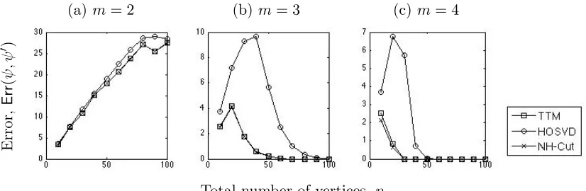
(a) m= 2 (b)m= 3 (c) m= 4
Error,
Err
(
ψ
,
ψ
0 )
Total number of vertices,n
Figure 1: Number of vertices mis-clustered by TTM, HOSVD and NH-Cut as n increases. The figures from left to right correspond to cases withm= 2, 3 and 4, respectively.
the setting of Corollary 3, and validates our theoretical observations about TTM. We next compare the performance of TTM with several uniform hypergraph partitioning methods for some small scale problems. The reason for restricting our study to small problems is because, in such cases, the hypergraphs can be completely specified, and edge sampling can be avoided. The rest of the section focuses on practical versions of the subspace clustering problem, where we compare sampled variants of TTM with state of the art subspace cluster-ing algorithms. Our experiments include both synthetic subspace clustercluster-ing problems (Park et al., 2014) and benchmark motion segmentation problem (Tron and Vidal, 2007).
6.1 Comparison of Spectral Algorithms
We first compare the performance of TTM with the HOSVD based algorithm (Govindu, 2005; Ghoshdastidar and Dukkipati, 2014) and the NH-Cut algorithm (Zhou et al., 2007; Ghoshdastidar and Dukkipati, 2017). This study is based on the model related to Corol-lary 3, where a m-uniform hypergraph is generated on n vertices. We assume here that αn = 1, k = 2, and the true clusters are of equal size. The edges occur with following probabilities. If all vertices in an edge do not belong to the same cluster, then the edge probability isq = 0.2, else it is (p+q) for some p∈(0,1−q) specified below.
In Figure 1, we show results for three examples, where p is fixed at p = 0.1, m is varied over m = 2,3,4, and the total number of vertices n grows from 10 to 100. For each case, 50 planted hypergraphs are generated, and subsequently partitioned by TTM, HOSVD and NH-Cut. The mean error, Err(ψ, ψ0), is reported for each algorithm as a function ofn. Figure 1 shows that the performance of TTM and NH-Cut are similar, and the errors incurred by these methods are significantly smaller than that of HOSVD. This observation validates Corollary 3 and Remark 5. It can also be seen empirically that all three methods have a sub-linear error rate for m = 2, i.e., they are weakly consistent, whereas,Err(ψ, ψ0) =o(1) for m≥3.
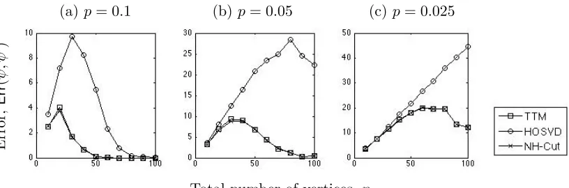
(a) p= 0.1 (b)p= 0.05 (c) p= 0.025
Error,
Err
(
ψ
,
ψ
0 )
Total number of vertices,n
Figure 2: Number of vertices mis-clustered by TTM, HOSVD and NH-Cut as n increases. The figures from left to right correspond to cases with p = 0.1, 0.05 and 0.025, respectively.
the problem becomes harder aspreduces, and the performance of HOSVD is highly affected. But, the effect is much less in case of TTM and NH-Cut. This follows from Theorem 2, where one can observe that, in the present contextErr(ψ, ψ0) varies as 1/p2. Same holds for NH-Cut, but in the case of HOSVD, Err(ψ, ψ0) varies as 1/p4 making the algorithm more sensitive to reduction in probability gap.
6.2 Comparison of Hypergraph Partitioning Methods
We consider similar studies with other hypergraph partitioning methods, such as methods based on symmetric non-negative tensor factorisation (SNTF) (Shashua et al., 2006), higher order game theoretic clustering (HGT) (Rota Bulo and Pelillo, 2013) and the hMETIS algorithm widely used in VLSI community (Karypis and Kumar, 2000). For the latter two methods, we have used implementations provided by the authors.
We first compare the different algorithms under a planted model for 3-uniform hyper-graphs with k= 3 planted clusters of equal size. As before, we assume the hypergraph to be dense,αn= 1, and the inter-cluster edges occur with probabilityq= 0.2. We study the performance of the methods as the number of vertices n, and the probability gapp varies. The fractional clustering error, n1Err(ψ, ψ0), averaged over 50 runs, is reported in Figure 3. The figure shows the previously observed trends for TTM, NH-Cut and HOSVD. In addition, it is observed that SNTF and hMETIS provide nearly similar, but marginally worse results than TTM. However, HGT uses a greedy strategy for extracting individual clusters, and hence, often identifies a majority of the vertices as outliers, thereby resulting in poor performance.
Probabilit
y
gap
p
Number of vertices in each cluster,n/k
Figure 3: Fractional error incurred by hypergraph partitioning algorithms under a planted model. The cluster size, (n/k), and the probability gapp are varied. The colour bar indicates the shade corresponding to different levels of error, with darker shade representing larger error.
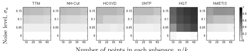
Noise
lev
el,
σa
Number of points in each subspace, n/k
Figure 4: Fractional error incurred by hypergraph partitioning algorithms in clustering noisy points from three intersecting lines. The cluster size, (n/k), and the noise levelσaare varied. The colour bar indicates the shade corresponding to different levels of error, with darker shade representing larger error.
noise vector to each point. The covariance of the noise vectors is given asσaI, where we vary σa to control the difficulty of the problem. We construct a weighted 3-uniform similarity hypergraph based on polar curvature of triplet of points, which is partitioned by the differ-ent methods. The fractional clustering errors are presdiffer-ented in Figure 4. As expected, all the methods can identify the exact subspace in the absence of noise, and the errors increase for larger σa. Apart from HGT, a good performance is observed from all the methods.
One can observe that the above comparisons were based on very small problems, where the hypergraph consists of at most 120 vertices. This restriction was imposed since speci-fication of the entire affinity tensor is computationally infeasible for large hypergraphs. To demonstrate the performance of TTM in practical settings, we study its sampled variants in the subsequent sections.
6.3 Comparison of Subspace Clustering Algorithms: Synthetic Data
not consider aforementioned hypergraph partitioning methods that require computation of the entire tensor. The clustering algorithms under consideration include:
• k-means algorithm for clustering based on Euclidean distance,
• k-flats algorithm (Bradley and Mangasarian, 2000) which generalisesk-means to sub-space clustering,
• sparse subspace clustering (SSC) (Elhamifar and Vidal, 2013), which finds clusters by estimating the subspaces,
• subspace clustering using low-rank representation (LRR) (Liu et al., 2010),
• thresholding based subspace clustering (TSC) (Heckel and B¨olcskei, 2013),
• faster variant of SSC using orthogonal matching pursuit (SSC-OMP) (Dyer et al., 2013),
• greedy subspace clustering using nearest subspace neighbour search and spectral clus-tering (NSN+Spectral) (Park et al., 2014),
• spectral curvature clustering (SCC) (Chen and Lerman, 2009), which is an iterative variant of HOSVD,
• sparse Grassmann clustering (SGC) (Jain and Govindu, 2013),8 yet another variation of HOSVD where some information about the eigenvectors computed in previous iterations is retained,
• Algorithm Tetris, and
• Algorithm TTM with uniform sampling, which is derived by performing a single iter-ation of Steps 1-14 of Algorithm Tetris.9
We first focus on the problem of clustering randomly generated subspaces.10 In an ambient space of dimensionra= 5, we randomly generatek= 5 subspaces each of dimension r = 3. From each subspace, we randomly samplen/k points and perturb every point with a 5-dimensional Gaussian noise vector with mean zero and covariance σaI. In Figure 5, we report the fractional error, n1Err(ψ, ψ0), incurred by various subspace clustering algorithms when (n/k) and σa are varied. The results are averaged over 50 independent trials. We note that for existing methods, we fix the parameters as mentioned in Park et al. (2014). For Tetris and SGC, the parameters are set to the same values as SCC, wherec= 100kand σ as in (31) is determined by the algorithm. In case of uniformly sampled TTM, we fix σ to be same as the value determined by Tetris. To demonstrate that sampling more edges lead to error reduction, we consider uniform sampling for two valuesc= 100kand 200k.
Figure 5 shows that Tetris and SGC clearly outperform other methods over a wide range of settings. In particular, it can be seen that greedy methods like NSN is accurate
8. For this method, we have used our implementation.
9. Here, the edge sampling is not exactly uniform since we only select thecsubsets of size (m−1) uniformly. 10. The experimental setup has been adapted from Park et al. (2014), and the codes are available at:
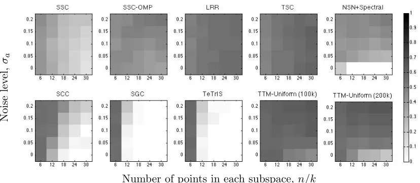
Noise
lev
el,
σa
Number of points in each subspace, n/k
Figure 5: Fractional error incurred by subspace clustering algorithms for synthetic data. The number of points in each subspace, (n/k), and the variance of the noise vector σa is varied. The colour bar indicates the shades for different levels of error.
in the absence of noise, but a drastic increase in error occurs when the data is noisy. The effect of noise is much less in hypergraph based methods like SCC, SGC or Tetris. One can also observe that the hypergraph based methods do not work well when there are very few points in each cluster (for example, 6). This is expected since, by definition, these algorithms construct 5-uniform hypergraphs (m = r + 2) in this case, and hence, there are very few edges ( 65 = 6) with large weight for each cluster. However, with increase in number of points, there is a rapid decay in the clustering error. This also shows the consistency of these methods empirically. To this end, it seems that NSN or SSC should be recommended for small scale problems (smaller n/k), whereas Tetris or SGC should be the algorithm of choice for larger nand possible presence of noise. Finally, we also observe that TTM with uniform sampling, even with twice the number of samples, performs quite poorly as compared to Tetris. However, with increase in the number of sampled edges, some extent of error reduction is observed.
6.4 Comparison of Subspace Clustering Algorithms: Motion Segmentation
The Hopkins 155 database (Tron and Vidal, 2007) contains a number of videos capturing motion of multiple objects or rigid bodies. In each video, few features are tracked along the frames, each giving rise to a motion trajectory that resides in a space of dimension twice the number of frames. One can show that under particular camera models, all trajectories corresponding to a particular rigid body motion span a subspace of dimension at most four (Tomasi and Kanade, 1992). Thus, the problem of segmenting different motions in a video can be posed as a subspace clustering problem.
Algorithm 2 motion (120 sequences) 3 motion (35 sequences) Mean (%) Median (%) Time (s) Mean (%) Median (%) Time (s) k-means 19.58 17.92 0.03 26.13 20.48 0.05
k-flats 13.19 10.01 0.38 15.45 14.88 0.76
SSC 1.53 0.00 0.80 4.40 0.56 1.51
LRR 2.13 0.00 0.94 4.03 1.43 1.29
SSC-OMP 16.93 13.28 0.72 27.61 23.79 1.23
TSC 18.44 16.92 0.19 28.58 29.67 0.51
NSN+Spec 3.62 0.00 0.08 8.28 2.76 0.17
SCC 2.53 0.03 0.45 6.40 1.46 0.76
SGC 3.50 0.41 0.54 9.08 5.05 0.89
Tetris 1.31 0.02 0.50 5.71 1.19 0.90
Table 1: Mean and median of clustering error and computational time for different subspace clustering algorithms on Hopkins 155 database.
motion segmentation. For existing approaches, the parameters specified in Park et al. (2014) have been used, and for Tetris and SGC, we use the parameters for SCC. TTM with uniform sampling is not considered due to its higher error rate. Table 1 reports the mean and median of the percentage errors incurred by different algorithms, where these statistics are computed over all 2-motion and 3-motion sequences. In order to remove the effect of randomisation due to sampling (for SCC, SGC, Tetris) or initialisation (fork-means,k-flats, NSN), we average the results over 20 independent trials. The average computational time (in seconds) of each algorithm for each video is also reported.11
Table 1 shows that Tetris performs quite well in comparison with state of the art sub-space clustering algorithms. In particular, Tetris achieves least mean error for the two motion problem. The computational time for Tetris is also much smaller than other accu-rate methods like SSC and LRR. The mean error achieved by Tetris is also smaller than SCC in either cases. We note here that the best known results for Hopkins 155 database is achieved by the algorithm in Jung et al. (2014), which uses techniques based on epi-polar geometry, and hence, it is not a subspace clustering algorithm. Smaller errors have also been reported in the literature when one construct larger tensors, m = 8 (Jain and Govindu, 2013), or uses manual tuning of hyper-parameters (Ghoshdastidar and Dukkipati, 2015a). However, in either cases, computational time increases considerably.
7. Conclusion
In this paper, we studied the problem of partitioning uniform hypergraphs that arises in several applications in computer vision and databases. We formalised the problem by defining a normalised associativity of a partition in a uniform hypergraph that extends a