The Thirty-Third AAAI Conference on Artificial Intelligence (AAAI-19)
A New Ensemble Learning Framework for 3D Biomedical Image Segmentation
Hao Zheng,
∗Yizhe Zhang,
∗Lin Yang,
∗Peixian Liang, Zhuo Zhao, Chaoli Wang, Danny Z. Chen
Department of Computer Science and Engineering, University of Notre Dame, Notre Dame, IN 46556, USA {hzheng3, yzhang29, lyang5, pliang, zzhao3, cwang11, dchen}@nd.edu
Abstract
3D image segmentation plays an important role in biomedi-cal image analysis. Many 2D and 3D deep learning models have achieved state-of-the-art segmentation performance on 3D biomedical image datasets. Yet, 2D and 3D models have their own strengths and weaknesses, and by unifying them to-gether, one may be able to achieve more accurate results. In this paper, we propose a newensemble learningframework for 3D biomedical image segmentation that combines the merits of 2D and 3D models. First, we develop a fully convo-lutional network based meta-learner to learn how to improve the results from 2D and 3D models (base-learners). Then, to minimize over-fitting for our sophisticated meta-learner, we devise a new training method that uses the results of the base-learners as multiple versions of “ground truths”. Furthermore, since our new meta-learner training scheme does not de-pend on manual annotation, it can utilize abundant unlabeled 3D image data to further improve the model. Extensive ex-periments on two public datasets (the HVSMR 2016 Chal-lenge dataset and the mouse piriform cortex dataset) show that our approach is effective under fully-supervised, semi-supervised, and transductive settings, and attains superior per-formance over state-of-the-art image segmentation methods.
1
Introduction
3D image segmentation plays an important role in biomed-ical image analysis (e.g., segmenting the whole heart to di-agnose cardiac diseases (Pace et al. 2015; Yu et al. 2017) and segmenting neuronal structures to identify cortical con-nectivity (Lee et al. 2015; Shen et al. 2017)). With recent rapid advances in deep learning, many 2D (Shen et al. 2017; Wolterink et al. 2017) and 3D (Yu et al. 2017; C¸ ic¸ek et al. 2016; Chen et al. 2017) convolutional neural networks (CNNs) have been developed to attain state-of-the-art seg-mentation results on various 3D biomedical image datasets (Pace et al. 2015; Shen et al. 2017). However, due to the lim-itations of both GPU memory and computing power, when designing 2D/3D CNNs for 3D biomedical image segmen-tation, the trade-off between the field of view and utilization of inter-slice information in 3D images remains a major con-cern. For example, 3D CNNs attempt to fully utilize 3D
im-∗
Equal contribution (Co-first authors). Author ordering deter-mined by dice rolling over a Google Hangout.
Copyright c2019, Association for the Advancement of Artificial Intelligence (www.aaai.org). All rights reserved.
age information but only have a limited field of view (e.g.,
64×64×64(Yu et al. 2017)), while 2D CNNs can have a much larger field of view (e.g.,572×572(Ronneberger, Fischer, and Brox 2015)) but are not able to fully explore inter-slice information.
Many methods have been proposed to circumvent this trade-off by carefully designing the structures of 2D and 3D CNNs. Their main ideas can be broadly classified into two categories. The models in the first category selectively choose the input data. For example, the tri-planar schemes (Wolterink et al. 2017; Prasoon et al. 2013) use only three orthogonal planes (i.e., thexy,yz, andxzplanes) instead of the whole 3D image, aiming to utilize inter-slice information without sacrificing the field of view. The models in the sec-ond category first summarize intra-slice information using 2D CNNs and then use the distilled information as an (extra) input to their 3D network component. For example, in (Lee et al. 2015), intra-slice information is first extracted using a 2D CNN (VD2D) and then passed to the 3D component (VD2D3D) via recursive training. In (Chen et al. 2016b), its recurrent neural network (RNN) component directly uses the results of 2D CNNs as input to compute 3D segmentation.
However, these methods still have considerable draw-backs. Tri-planar schemes (Wolterink et al. 2017; Prasoon et al. 2013) use only a small fraction of 3D image infor-mation and the computation cost is not reduced but shifted to the inference stage (a tri-planar scheme can only predict one voxel at a time, which is very slow when predicting new 3D images). For models that first summarize intra-slice in-formation, the asymmetry nature of the network design (first 2D, then 3D) may hinder a full utilization of 3D image infor-mation (2D results may dominate since they are much easier to be interpreted than raw images in the 3D stage).
In this paper, we explore a different perspective. Instead of designing new network structures to circumvent the trade-off between field of view and inter-slice information, we ad-dress this difficulty by developing a newensemble learning
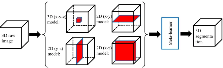
framework for 3D biomedical image segmentation which aims to retain and combine the merits of 2D/3D models. Fig. 1 gives an overview of our framework.
im-3D raw image
3D (x-y-z) model:
2D (y-z) model:
2D (x-y) model:
2D (x-z) model:
Met
a-le
ar
ne
r
3D segmenta tion
Figure 1: An overview of our proposed framework. Red box/planes show the effective fields of view of the corresponding 3D/2D base-learners. Our meta-learner works on top of all the base-learners.
age samples, X = {x1, x2, . . . , xn}, their correspond-ing ground truth, Y = {y1, y2, . . . , yn}, and a set of base-learners, F = {f1, f2, . . . , fm}, a common design of a meta-learner is to learn the prediction of (xi,yi)ˆ =
fmeta(f1(xi), f2(xi), . . . , fm(xi)), by fittingyi. Since the
results from the base-learners can be very close to the ground truth, training the meta-learner by directly fittingyi is
sus-ceptible to over-fitting. Many measures have been proposed to address this issue: (1) simple meta-learner structure de-signs (e.g., in (Ju, Bibaut, and van der Laan 2018), the meta-learner was implemented as a single1×1convolution layer, and in (Makarchuk et al. 2018), the meta-learner was im-plemented using the XGBoost classifier (Chen and Guestrin 2016)); (2) excluding raw image information from the in-put (Zhou 2012); (3) splitting the training data into multiple folds and training the meta-learner by minimizing the cross-validated risk (Van der Laan, Polley, and Hubbard 2007).
However, in our 3D biomedical image segmentation sce-nario, these meta-learner designs may not work well due to the following reasons. First, each of our individual base-learners (2D and 3D models) has its distinct merit; in many difficult image areas, it is quite likely that only one of the base-learners could produce the correct results. Thus, our meta-learner should be sophisticated enough in order to cap-ture the merits of all the base-learners. Second, since ex-tensive annotation efforts are often needed to produce full 3D annotation, not many 3D training images are available (e.g., 3 in (Lee et al. 2015) and 10 in (Pace et al. 2015)) in common 3D biomedical image datasets. Splitting the al-ready scarce training data can largely lower the accuracy of the base-learners and meta-learner.
Hence, we propose a new stacking method that includes (1) a deep learning based meta-learner to combine and im-prove the results of the base-learners, and (2) a new learner training method that can train a sophisticated meta-learner with less risk of over-fitting.
A deep learning based meta-learner.Comparing with
image classification, the output domain of image segmenta-tion is much more structural. However, recent studies have not leveraged this property to design a better meta-learner for image segmentation. For example, in (Ju, Bibaut, and van der Laan 2018; Nigam, Huang, and Ramanan 2018), only linear combination of base-learners was explored. We develop a new fully convolutional network (FCN) based
meta-learner to capture the merits of our base-learners and produce spatially consistent results.
Minimizing the risk of over-fitting.A key idea of our
meta-learner training method is to use the results of the base-learners aspseudo-labels (Lee 2013) and compute ensem-ble by finding a balance among these pseudo-labels through the training process (in contrast to directly fittingyi). More specifically, for each input samplexi, there are multiple ver-sions of pseudo-labels (from the individual base-learners). During the iterative meta-learner training process, in each iteration, we randomly choose one pseudo-label from all the versions and use it as “ground truth” to compute the loss and update meta-learner parameters. Iteration by iteration, the pseudo-labels with small disagreement would provide a more consistent supervision and the pseudo-labels with large disagreement would request the meta-learner to find a bal-anced solution by minimizing the overall loss.
Our method can minimize the risk of over-fitting in two aspects. (1) Intuitively, over-fitting occurs when a model over-explains the ground truth. Since our method uses mul-tiple versions of “ground truths” (pseudo-labels), the meta-learner is unlikely to over-fit any one of them. (2) Since our meta-learner training uses only model-generated results, un-labeled data can be easily incorporated into the training pro-cess; this will allow us to further reduce over-fitting.
Compared with previous methods that combine 2D and 3D models, our main contributions are: (a) a new ensem-ble learning framework for tackling 3D biomedical image segmentation from a different perspective, and (b) an ef-fective meta-learner training method for ensemble learn-ing that minimizes the risk of over-fittlearn-ing and makes use of unlabeled data. Extensive experiments on two pub-lic datasets (the HVSMR 2016 Challenge dataset (Pace et al. 2015) and the mouse piriform cortex dataset (Lee et al. 2015)) show that our framework is effective un-der fully-supervised, semi-supervised, and transductive set-tings, and attains superior performance over the state-of-the-art methods (Yu et al. 2017; Shen et al. 2017; Chen et al. 2017). Code will be made publicly available at https://github.com/HaoZheng94/Ensemble.
2
Method
the training data from different geometric perspectives; (2) an ensemble learning framework that uses a deep learning based meta-learner to combine the results from the base-learners. A schematic overview of our proposed framework is shown in Fig. 1.
In Section 2.1, we illustrate how to design our 2D and 3D base-learners to achieve a set of accurate and diverse re-sults. In Section 2.2, we discuss our new deep learning based meta-learner that can considerably improve the results from the base-learners. In Section 2.3, we present our new method for training a more powerful meta-learner while preventing over-fitting.
2.1
2D and 3D base-learners
To achieve the best possible ensemble results, it is com-monly desired that individual base-learners be asaccurate
and asdiverseas possible (Zhou 2012). In this section, we show how to design our 2D and 3D base-learners to satisfy these two criteria.
For accurate results.Our 2D model basically follows the
structure of that in (Yang et al. 2017). We choose this struc-ture because it is based on a well-known FCN (Chen et al. 2016a) which has attained lots of successes in biomedical image segmentation and has been integrated in recent ad-vances of deep learning network design structures, such as batch normalization (Ioffe and Szegedy 2015), residual net-works and bottleneck design (He et al. 2016). It generalizes well and is fast to train. As for the 3D model, we use Den-seVoxNet (Yu et al. 2017), for three reasons. First, it adopts a 3D FCN architecture, and thus can fully incorporate 3D im-age cues and geometric cues for effective volume-to-volume prediction. Second, it utilizes the state-of-the-art dense con-nectivity (Huang et al. 2017) to accelerate the training pro-cess, improve parameters and computational efficiency, and maintain abundant (both low- and high-complexity) features for segmenting complicated biomedical structures. Third, it takes advantage of auxiliary side paths for deep supervision (Dou et al. 2016) to improve the gradient flow within the network and stabilize the learning process. For further de-tails of these 2D and 3D models, the readers are referred to (Yang et al. 2017) and (Yu et al. 2017).
For diverse results.Our key idea to achieve diverse
re-sults is to let each of our base-learners have a unique geomet-ric view of the data. As discussed in Section 1, 2D models can have large fields of view in 2D slices while 3D models can better utilize 3D image information in a smaller field of view. Our mix of 2D and 3D base-learners creates the first level of diversity. To further boost diversity, within the group of 2D base-learners, we leverage the 3D image data to create multiple 2D views (representations) of the 3D images (e.g.,
xy,xz, andyzviews). The different 2D representations of the 3D images create 2D models with diverse strengths (e.g., large fields of view for different planes) and thus generate diverse 2D results. Note that the 2D representations are not limited to being orthogonal to each of the major axes. But, based on our trial studies, we found that the results from the
xy, xz, andyz views are the most accurate (probably be-cause no interpolation is needed when extracting these 2D slices from 3D images) and already create good diversity.
Thus, in our framework, we use the following four base-learners: a 3D DenseVoxNet (Yu et al. 2017) for utilizing full 3D information; three 2D FCNs (Yang et al. 2017) for large fields of view in thexy,xz, andyzplanes.
2.2
Deep meta-learner structure design
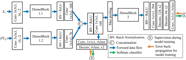
Since our base-learners have distinct model architectures and work on different geometric perspectives of 3D im-ages to produce diverse predictions, for difficult image ar-eas, there is a better chance that one of the base-learners would give correct predictions (see Fig. 3). In order to attain a meta-learner to pick up the correct predictions, we need a model that is, architecture and complexity wise, capable of learning robust visual features for jointly utilizing the di-verse prediction results (from the base-learners) as well as the raw image information. It is known that simple models (e.g., linear models, shallow neural networks) are not pow-erful enough to learn/extract robust and comprehensive fea-tures for difficult vision tasks (Zhou 2012). Furthermore, our learning task is a segmentation problem that requires spa-tially consistent output. Thus, we employ a state-of-the-art 3D FCN (DenseVoxNet (Yu et al. 2017)) for building our meta-learner. The input of the network is the base-learners’ results and the raw image, and the output of the network is the computed ensemble. Below we describe how to con-struct the input of our deep meta-learner and the details of the deep meta-learner’s model architecture.
Given a set of image samples, X = {x1, x2, . . . , xn}, and a set of base-learners, F = {f1, f2, . . . , fm}, a
pseudo-label set for each xi can be obtained as P Li =
{f1(xi), f2(xi), . . . , fm(xi)}. The input of our meta-learner
Hincludes two parts:xi andS(P Li), where S is a func-tion ofP Li that forms a representation ofP Li. There are
multiple design choices for constructingS. For example, (1) concatenating all the elements ofP Li, or (2) averaging all the elements ofP Li. Concatenation allows the meta-learner
to gain full information from the base-learners (no informa-tion is added or lost). Averaging provides a more compact representation of all pseudo-labels, while still showing the image areas where the pseudo-labels hold agreement or dis-agreement. Furthermore, using the average of all the pseudo-labels ofxi to form part of the meta-learner’s input can be viewed as a preliminary ensemble of the base-learners. We have experimented with both these design choices and found that makingSan averaging function of the elements ofP Li
gives slightly better results. The overall model specification of our proposed deep meta-learner is shown in Fig. 2.
2.3
Meta-learner training using pseudo-labels
Co nv 3x3x3 , 16, /2 B N + Re L U Co nv 1x1x1 , 1 60 Ma x po ol in g BN + Re L U Co nv 1x1x1 , 3 04 De co nv , 1 28 , x 2 De co nv , 6 4, x 2 DenseBlock 1.1
BN: Batch Normalization
Forward data flow
Concatenation Co nv 3x3x3 , 16, /2 B N + Re L U Co nv 1x 1x1 , 7 6 C BN + Re L U Co nv 1x1x1 , 160
Deconv, #class, x2 C
S
S
S Supervision during model training Error back-propagation for model training DenseBlock 1.2 DenseBlock 2 Concatenation Conv, 1x1x1, #class
C
onv
, 1x1x1, #c
la
ss
Softmax classifier xi
S(PLi)
Figure 2: Our deep meta-learner (a variant of 3D DenseVoxNet (Yu et al. 2017)). SinceS(P Li)andxiare of different nature, we use separate encoding blocks (i.e., DenseBlock 1.1 and DenseBlock 1.2) for extracting information fromS(P Li)andxi, respectively, before the information fusion. The auxiliary loss in the side path can improve the gradient flow within the network.
for unlabeled data. Thus, our method is also capable of us-ing unlabeled data for deep meta-learner trainus-ing (which can further reduce over-fitting).
Suppose X, P Li, and S(P Li) are given, for i = 1,2, . . . , n. Ideally, the learning objective of the meta-learner would be: (1) finding the “best” pseudo-labels in
P Li, and (2) training the meta-learnerHto fit the pseudo-labels found in (1). However, the best pseudo-pseudo-labels are not clearly defined and can be difficult to find. Based on different evaluation criteria, the “best” choices can be different. Even when a criterion is given, using the most accurate pseudo-labels can likely lead to a higher chance of suffering over-fitting. Furthermore, when training using unlabeled data, it is in general quite difficult to determine which pseudo-label gives more accurate predictions than the others. One could set up a hand-crafted algorithm based on a predefined cri-terion to select the “best” pseudo-labels for training. The meta-learner, however, could very likely over-fit the algo-rithm’s choices and hence likely not be able to generalize well to future unseen image data.
Rather than explicitly defining the full learning objec-tive for learner training, we initially train the meta-learner in order to set up a near-optimal (or sub-optimal) configuration: The meta-learner is aware of all the avail-able pseudo-labels, and its position in the hypothesis space is influenced by the raw image and the pseudo-label data distribution. Next, the meta-learner itself chooses the near-est pseudo-labels to fit (based on its current model param-eters) and updates its model parameters based on its cur-rent choices. This nearest-neighbor-fit process iterates un-til the meta-learner fits the nearest neighbors well enough. Thus, our meta-learner training consists of two phases: (1) random-fit, and (2) nearest-neighbor-fit. We describe these two training phases below.
Random-fit. In the first training phase (which aims to
train the meta-learnerHto reach a near-optimal solution), we seek to minimize the overall cross-entropy loss for all the image samples with respect to all the pseudo-labels:
`(θH)=
n X i=1 m X j=1
`mce(θH(xi, S(P Li)),fj(xi)), (1)
whereθHis the meta-learner’s model parameters and`mceis
a multi-class cross-entropy criterion. The above loss ensures
Algorithm 1:Random-fit
Input:(xi, P Li ={f1(xi), f2(xi), . . . ,
fm(xi)}, S(P Li)), i= 1,2, . . . , n;
Output:A trained meta-learnerH;
initialize a meta-learnerHwith random weights; mini-batch =∅;
whilestopping condition not metdo
fork= 1 to batch-sizedo p=rand-int(1, n);
q=rand-int(1, m);
add training sample{(xp, S(P Lp)), fq(xp)}to the mini-batch;
updateHusing training samples in the mini-batch with forward and backward propagation; mini-batch =∅;
that the meta-learner training process in this phase works on all the available pseudo-labels. Since the loss function itself does not impose any favor towards any particular pseudo-labels produced by the base-learners, our meta-learner is unlikely to over-fit any pseudo-labels. Exploring the overall raw image and the pseudo-label data distribution, the meta-learner obtained by minimizing the above loss may have dif-ferent tendencies towards difdif-ferent pseudo-labels.
To effectively optimize the loss function in Eq. (1), we develop a random-fit algorithm. In the SGD-based opti-mization, for one image samplexi, our algorithm randomly chooses a pseudo-label from P Li and sets it as the
cur-rent “ground truth” forxi (see Algorithm 1). This ensures the supervision signals not to impose any bias towards any base-learner, and allows image samples with diverse pseudo-labels to have a better chance to be influenced by other im-age samples. Our experiments show that our random-fit al-gorithm is effective for learning with diverse pseudo-labels.
Nearest-neighbor-fit (NN-fit). Unlike image
Algorithm 2:Nearest-neighbor-fit (NN-fit)
Input:(xi, P Li={f1(xi), f2(xi), . . . ,
fm(xi)}, S(P Li)), i= 1,2, . . . , n, meta-learnerH(obtained from random-fit);
Output:A refined meta-learnerH;
mini-batch =∅;
whilestopping condition not metdo
fork= 1 to batch-sizedo p=rand-int(1, n);
ˆ
y=H(xp, S(P Lp));
ˆ
q= arg minq=1,2,...,mLmce(ˆy, fq(xp));
add training sample{(xp, S(P Lp)), fqˆ(xp)}to the mini-batch;
updateHusing training samples in the mini-batch with forward and backward propagation; mini-batch =∅;
raw image average ensemble random-fit NN-fit
2D xy base-learner 2D xz base-learner 2D yz base-learner 3D base-learner
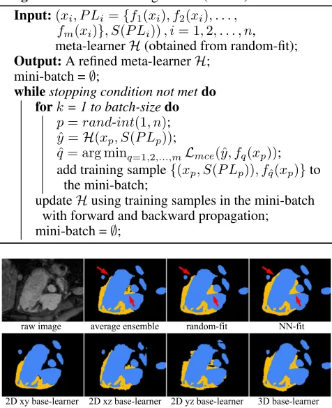
Figure 3: Visual comparison of segmentation results (yel-low: myocardium; blue: blood pool). With NN-fit, our meta-learner can achieve more accurate segmentation of my-ocardium (red arrows).
incorrect. Even when all pseudo-labels of a particular im-age sample are close to the true solution, the trained meta-learner, if not fitting any of the pseudo-labels appropriately, can still have a risk of producing new types of errors.
Thus, to help the model training process converge, in the second training phase, we aim to train the meta-learner to fit the nearest pseudo-label. Since the overall training loss is based on cross-entropy, to make NN-fit have direct effects on the convergence of the model training, we use cross-entropy to measure difference between a meta-learner’s output and a pseudo-label. The details of our NN-fit algorithm are pre-sented in Algorithm 2. Our experiments show that NN-fit can effectively improve the performance of the deep meta-learner (see Fig. 3, and Tables 1 and 2).
3
Evaluation datasets and implementation
details
We evaluate our approach using two public datasets: (1) the HVSMR 2016 Challenge dataset (Pace et al. 2015) and (2) the mouse piriform cortex dataset (Lee et al. 2015).
HVSMR 2016.The objective of the HVSMR 2016
Chal-lenge (Pace et al. 2015) is to segment the myocardium and great vessel (blood pool) in cardiovascular magnetic res-onance (MR) images. 10 3D MR images and their
corre-sponding ground truth annotation are provided by the chal-lenge organizers as training data. The test data, consist-ing of another 10 3D MR images, are publicly available, yet their ground truths are kept secret for fair comparison. The results are evaluated using three criteria: (1) Dice co-efficient, (2) average surface distance (ADB), and (3) sym-metric Hausdorff distance. Finally, a scoreS, computed as
S = P class(
1 2Dice−
1 4ADB−
1
30Hausdorff), is used to reflect the overall accuracy of the results and for ranking.
Mouse piriform cortex.Our approach is also evaluated
on the mouse piriform cortex dataset (Lee et al. 2015) for neuron boundary segmentation in serial section EM images. This dataset contains 4 stacks of 3D EM images. Following the previous practice (Lee et al. 2015; Shen et al. 2017), the 2nd, 3rd, and 4th stacks are used for model training, and the 1st stack is used for testing. Also, as in (Lee et al. 2015; Shen et al. 2017), the results are evaluated using the Rand F-score (the harmonic mean of the Rand merge F-score and the Rand split score).
Implementation details. All our networks are
imple-mented using TensorFlow (Abadi et al. 2016). The weights of our 2D base-learners are initialized using the strategy in (He et al. 2015). The weights of our 3D base-learner and meta-learner are initialized with a Gaussian distribution (µ= 0,σ= 0.01). All our networks are trained using Adam (Kingma and Ba 2015) with β1 = 0.9,β2 = 0.999, and
=1e-10. The initial learning rates are all set as 5e-4. Our 2D base-learners reduce the learning rates to 5e-5 after 10k iterations; our 3D base-learner and meta learner adopt the “poly” learning rate policy (Yu et al. 2017) with the power variable equal to 0.9 and the max iteration number equal to 40k. To leverage the limited training data, standard data aug-mentation techniques (i.e., random rotation with 90, 180, and 270 degrees, as well as image flipping along the axial planes) are employed to augment the training data.
For the HVSMR 2016 Challenge dataset, due to large in-tensity variance among different images, all the cardiac im-ages are normalized to have zero mean and unit variance. We also employ spatial resampling to 1mm isotropically. For the mouse piriform cortex data, since the 3D EM images are highly anisotropic (7×7×40nm), the 2D base-learners in thexz andyzviews did not converge well. Thus, we only use the 3D base-learner and the 2D base-learner in the xy
view for this dataset.
4
Experiments
Because our meta-learner training does not require any manual-labeled data, our method can be easily adapted to the semi-supervised and transductive settings. Thus, we experi-ment with the following three main settings to demonstrate the effectiveness of our method.
1. To achieve fair comparison with the known state-of-the-art methods that cannot leverage unlabeled data, under the first setting, we train our meta-learner using only training data (the “only training data” entries in Tables 1 and 2).
Table 1: Quantitative analysis on the HVSMR 2016 dataset. VFN∗: For fair comparison, we use DenseVoxNet (Yu et al. 2017) as backbone, which is the same as our 3D base-learner.
Method Myocardium Blood pool Overallscore
Dice ADB [mm] Hausdorff [mm] Dice ADB [mm] Hausdorff [mm] 3D U-Net (C¸ ic¸ek et al. 2016) 0.694±0.076 1.461±0.397 10.221±4.339 0.926±0.016 0.940±0.192 8.628±3.390 -0.419 VoxResNet (Chen et al. 2017) 0.774±0.067 1.026±0.400 6.572±0.013 0.929±0.013 0.981±0.186 9.966±3.021 -0.202 DenseVoxNet (Yu et al. 2017) 0.821±0.041 0.964±0.292 7.294±3.340 0.931±0.011 0.938±0.224 9.533±4.194 -0.161 Wolterinket al.(Wolterink et al. 2017) 0.802±0.060 0.957±0.302 6.126±3.565 0.926±0.018 0.885±0.223 7.069±2.857 -0.036 VFN∗(Xia et al. 2018) 0.773±0.098 0.877±0.318 4.626±2.319 0.935±0.009 0.770±0.098 5.420±2.152 0.108 Base learner 2D (xy) 0.789±0.076 0.852±0.265 4.231±1.908 0.930±0.016 0.794±0.153 5.295±1.671 0.13 Base learner 2D (xz) 0.736±0.093 1.000±0.260 5.417±1.604 0.924±0.015 0.932±0.113 7.951±2.820 -0.098 Base learner 2D (yz) 0.756±0.082 0.870±0.181 4.169±0.632 0.928±0.012 0.812±0.111 5.229±1.721 0.108 Base learner 3D 0.809±0.069 0.785±0.235 4.121±1.870 0.937±0.008 0.799±0.145 6.285±3.108 0.13 Average ensemble 0.805±0.073 0.708±0.184 3.211±0.923 0.936±0.011 0.752±0.119 5.960±2.526 0.2
Our meta-learner
(only training data) 0.823±0.060 0.685±0.164 3.224±1.096 0.935±0.010 0.763±0.120 5.804±2.670 0.21 Our meta-learner
(transductive) 0.833±0.054 0.681±0.178 3.285±1.370 0.939±0.008 0.733±0.143 5.670±2.808 0.234
3. We show that improved results can be obtained under the tranductive setting in which we allow our meta-learner to utilize test data (the “transductive” entries in Tables 1 and 2). We emphasize that, although it might be less common to use test data for training in natural scene image seg-mentation, the transductive setting plays an important role in many biomedical image segmentation tasks (e.g., for making biomedical discoveries). For example, after bio-logical experiments are finished, one may have all the raw images available and the sole remaining goal is to train a model to attain the best possible segmentation results for all the data to achieve accurate quantitative analysis.
4.1
Comparison with state-of-the-art methods
when only using training data
HVSMR 2016. Table 1 shows a quantitative comparison
with other methods in the leader board of the HVSMR 2016 Challenge (Pace et al. 2015). Recall the two categories of the known deep learning based 3D segmentation methods (discussed in Section 1). We choose at least one typical method from each category for comparison. (1) (Wolterink et al. 2017) is based on the tri-planar scheme (Prasoon et al. 2013), which utilizesthree2D ConvNets on the orthogonal planes to predict a class label for each voxel. (2) VFN (Xia et al. 2018) first trainsthree2D models with slices that are split from three orthogonal planes, respectively, and then ap-plies a 3D ConvNet to fuse 2D results together. Besides, we compare our approach with state-of-the-art models (includ-ing 3D U-Net (C¸ ic¸ek et al. 2016), VoxResNet (Chen et al. 2017), and DenseVoxNet (Yu et al. 2017)). Without using unlabeled data, our meta-learner outperforms these meth-ods on nearly all the metrics and has a very high overall score, 0.215 (ours)vs.−0.161(DenseVoxNet),−0.036 (tri-planar), and0.108(VFN).
Mouse piriform cortex.Owning to the advanced
compo-nents used in our base-learners (e.g., ResNet compocompo-nents (He et al. 2016) and DenseNet components (Huang et al. 2017)), our 2D and 3D base-learners already achieve bet-ter results than the known state-of-the-art methods (Table
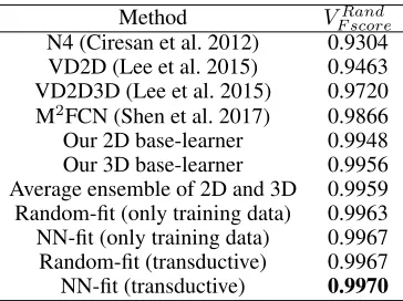
Table 2: Quantitative results on the mouse piriform cortex dataset.
Method VF scoreRand
N4 (Ciresan et al. 2012) 0.9304 VD2D (Lee et al. 2015) 0.9463 VD2D3D (Lee et al. 2015) 0.9720 M2FCN (Shen et al. 2017) 0.9866 Our 2D base-learner 0.9948 Our 3D base-learner 0.9956 Average ensemble of 2D and 3D 0.9959 Random-fit (only training data) 0.9963 NN-fit (only training data) 0.9967 Random-fit (transductive) 0.9967 NN-fit (transductive) 0.9970
2). Nevertheless, from Table 2, one can see that our meta-learner is able to (1) further improve the accuracy of the base-learners, and (2) achieve a result that is considerably better than the known state-of-the-art methods (0.9967 vs.
0.9866).
4.2
Utilizing unlabeled data
Semi-supervised setting. We conduct semi-supervised
learning experiments on the HVSMR 2016 dataset. The training set of HVSMR 2016 is randomly divided into two groups evenly,Sa andSb. We conduct two sets of experi-ments. Under the setting of “Group A”, we first useSa to
Table 3: Ablation experiments on the HVSMR 2016 dataset. “GT” represents ground truth and “PL” represents pseudo labels. Transductive learning setting: Test image data are involved as unlabeled data in model training.
Setting Inputs Supervision of training set
Transductive learning
Supervision of testing set
Training Overall score
raw image (xi) S(P Li) random fit NN fit
S1 3 GT 0.075
S2 3 3 GT 0.192
S3 3 3 GT 3 PL 3 0.217
S4 3 3 GT + PL 3 PL 3 0.205
S5 3 3 GT + PL 3 PL 3 3 0.224
S6 3 3 PL 3 0.199
S7 3 3 PL 3 3 0.215
S8 3 3 PL 3 PL 3 0.218
S9 3 3 PL 3 PL 3 3 0.234
Transductive setting.In this setting, we use the full
train-ing data to train our base learners, and use the traintrain-ing and testing data to train our meta-learner. As discussed at the beginning of this section, the transductive setting is impor-tant for biomedical image segmentation applications and re-search. The ability to refine the model after seeing the raw test data (no annotation for test data) is another advantage of our framework. From Table 1 and Table 2, one can see that our meta-learner can achieve further improvements than us-ing only the trainus-ing data (0.234vs.0.215 on the HVSMR dataset, and 0.9970vs.0.9967 on the piriform dataset).
4.3
Ablation study
Average ensemblevs.na¨ıve meta-learnervs.our best.The
results of the average ensemble of all the base-learners (the 2D and 3D models) are shown in Tables 1 and 2. One can see that the average ensemble is consistently worse than our meta-learner ensemble. We also compare our meta-learner with the na¨ıve meta-learner implementation (in which the outputs of the base-learners are used as input and the ground truths of the training set are used to train the meta-learner). Table 3 shows the results (the S1 row). One can see that the na¨ıve meta-learner implementation is even worse than the average ensemble (probably due to over-fitting). This demonstrates the effectiveness of our meta-learner structure design and training strategy.
Random-fit + NN-fitvs.Random-fit alone.Random-fit +
NN-fit performs significantly better than Random-fit alone (Table 3: S7>S6, S5>S4, S9>S8; Table 2), which demon-strates that NN-fit can help the training procedure converge and thus improve the segmentation quality.
Model training using pseudo-labelsvs.ground truth.One
may concern that our meta-learner training method totally discards manual-labeled ground truth even when it is avail-able. This ablation study shows that our method can perform better without using any manual ground truth. We explore the following ways of utilizing ground truth. When using only the training data, we compare the difference between only ground truth (S2) and only pseudo-labels (S7). Table 3 shows that our training method can achieve better results (0.215>0.192) when not using ground truth. When utiliz-ing the test data (the transductive settutiliz-ing), we compare the difference between (1) only ground truth (S3), (2) mix of ground truth and pseudo-labels, i.e., using ground truth as
Table 4: Semi-supervised setting on HVSMR 2016 dataset.
Group Model Overall score
A Base-learner 3D -0.036 Meta-learner 0.063
B Base-learner 3D -0.045 Meta-learner 0.038
the 5th version (S4 & S5), and (3) only pseudo-labels (S8 & S9). In Table 3, one can see that (a) using pure ground truth or pure pseudo-labels achieves better results than mix-ing them together (probably due to the different nature of ground truth and labels), and (b) using only pseudo-labels is still better than using ground truth (S8>S3). We think the reason that our method can work well with only pseudo-labels is because the pseudo-labels have already ef-fectively distilled the knowledge from ground truth (Hinton, Vinyals, and Dean 2015).
5
Conclusions
In this paper, we presented a newensemble learning frame-work for 3D biomedical image segmentation that can retain and combine the merits of 2D and 3D models. Our approach consists of (1) diverse and accurate base-learners by lever-aging diverse geometric and model-architecture perspectives of multiple 2D and 3D models, (2) a fully convolutional net-work (FCN) based meta-learner that is capable of learning robust visual features/representations to improve the base-learners’ results, and (3) a new meta-learner training method that can minimize the risk of over-fitting and utilize unla-beled data to improve performance. Extensive experiments on two public datasets show that our approach can achieve superior performance over the state-of-the-art methods.
6
Acknowledgments
This research was supported in part by the U.S. Na-tional Science Foundation through grants CCF-1617735, IIS-1455886, and CNS-1629914.
References
2016. TensorFlow: A system for large-scale machine learn-ing. InOSDI, volume 16, 265–283.
Chen, T., and Guestrin, C. 2016. XGBoost: A scalable tree boosting system. InKDD, 785–794.
Chen, H.; Qi, X.; Yu, L.; and Heng, P.-A. 2016a. DCAN: Deep contour-aware networks for accurate gland segmenta-tion. InCVPR, 2487–2496.
Chen, J.; Yang, L.; Zhang, Y.; Alber, M.; and Chen, D. Z. 2016b. Combining fully convolutional and recurrent neural networks for 3D biomedical image segmentation. InNIPS, 3036–3044.
Chen, H.; Dou, Q.; Yu, L.; Qin, J.; and Heng, P.-A. 2017. VoxResNet: Deep voxelwise residual networks for brain segmentation from 3D MR images.NeuroImage.
C¸ ic¸ek, ¨O.; Abdulkadir, A.; Lienkamp, S. S.; Brox, T.; and Ronneberger, O. 2016. 3D U-Net: Learning dense volu-metric segmentation from sparse annotation. In MICCAI, 424–432.
Ciresan, D.; Giusti, A.; Gambardella, L. M.; and Schmid-huber, J. 2012. Deep neural networks segment neuronal membranes in electron microscopy images. InNIPS, 2843– 2851.
Dou, Q.; Chen, H.; Jin, Y.; Yu, L.; Qin, J.; and Heng, P.-A. 2016. 3D deeply supervised network for automatic liver segmentation from CT volumes. InMICCAI, 149–157. He, K.; Zhang, X.; Ren, S.; and Sun, J. 2015. Delving deep into rectifiers: Surpassing human-level performance on Im-ageNet classification. InICCV, 1026–1034.
He, K.; Zhang, X.; Ren, S.; and Sun, J. 2016. Deep residual learning for image recognition. InCVPR, 770–778. Hinton, G.; Vinyals, O.; and Dean, J. 2015. Distilling the knowledge in a neural network. InNIPS Deep Learning and Representation Learning Workshop.
Huang, G.; Liu, Z.; Weinberger, K. Q.; and van der Maaten, L. 2017. Densely connected convolutional networks. In
CVPR, 2261–2269.
Ioffe, S., and Szegedy, C. 2015. Batch normalization: Accel-erating deep network training by reducing internal covariate shift. arXiv preprint arXiv:1502.03167.
Ju, C.; Bibaut, A.; and van der Laan, M. 2018. The relative performance of ensemble methods with deep convolutional neural networks for image classification.Journal of Applied Statistics1–19.
Kingma, D. P., and Ba, J. 2015. Adam: A method for stochastic optimization. InICLR.
Lee, K.; Zlateski, A.; Ashwin, V.; and Seung, H. S. 2015. Recursive training of 2D-3D convolutional networks for neuronal boundary prediction. InNIPS, 3573–3581. Lee, D.-H. 2013. Pseudo-label: The simple and efficient semi-supervised learning method for deep neural networks. In Workshop on Challenges in Representation Learning, ICML, volume 3, 2.
Makarchuk, G.; Kondratenko, V.; Pisov, M.; Pimkin, A.; Krivov, E.; and Belyaev, M. 2018. Ensembling neural
net-works for digital pathology images classification and seg-mentation.arXiv preprint arXiv:1802.00947.
Nigam, I.; Huang, C.; and Ramanan, D. 2018. Ensemble knowledge transfer for semantic segmentation. In WACV, 1499–1508.
Pace, D. F.; Dalca, A. V.; Geva, T.; Powell, A. J.; Moghari, M. H.; and Golland, P. 2015. Interactive whole-heart seg-mentation in congenital heart disease. InMICCAI, 80–88. Prasoon, A.; Petersen, K.; Igel, C.; Lauze, F.; Dam, E.; and Nielsen, M. 2013. Deep feature learning for knee cartilage segmentation using a triplanar convolutional neural network. InMICCAI, 246–253.
Ronneberger, O.; Fischer, P.; and Brox, T. 2015. U-Net: Convolutional networks for biomedical image segmentation. InMICCAI, 234–241.
Shen, W.; Wang, B.; Jiang, Y.; Wang, Y.; and Yuille, A. 2017. Multi-stage multi-recursive-input fully convolutional networks for neuronal boundary detection. InICCV, 2391– 2400.
Van der Laan, M. J.; Polley, E. C.; and Hubbard, A. E. 2007. Super learner. Statistical Applications in Genetics and Molecular Biology6(1).
Wolpert, D. H. 1992. Stacked generalization. Neural Net-works5(2):241–259.
Wolterink, J. M.; Leiner, T.; Viergever, M. A.; and Iˇsgum, I. 2017. Dilated convolutional neural networks for cardio-vascular MR segmentation in congenital heart disease. In
Reconstruction, Segmentation, and Analysis of Medical Im-ages, 95–102.
Xia, Y.; Xie, L.; Liu, F.; Zhu, Z.; Fishman, E. K.; and Yuille, A. L. 2018. Bridging the gap between 2D and 3D organ segmentation. arXiv preprint arXiv:1804.00392.
Yang, L.; Zhang, Y.; Chen, J.; Zhang, S.; and Chen, D. Z. 2017. Suggestive annotation: A deep active learning frame-work for biomedical image segmentation. InMICCAI, 399– 407.
Yu, L.; Cheng, J.-Z.; Dou, Q.; Yang, X.; Chen, H.; Qin, J.; and Heng, P.-A. 2017. Automatic 3D cardiovascular MR segmentation with densely-connected volumetric ConvNets. InMICCAI, 287–295.