Robust Negative Sampling for Network Embedding

(1)

The Thirty-Third AAAI Conference on Artificial Intelligence (AAAI-19)

Robust Negative Sampling for Network Embedding

Mohammadreza Armandpour,

1

Patrick Ding,

1

Jianhua Huang,

1

Xia Hu

2 1_{Department of Statistics, Texas A&M University}

2_{Department of Computer Science and Engineering, Texas A&M University}

{armand, patrickding, jianhua}@stat.tamu.edu, [email protected]

Abstract

Many recent network embedding algorithms use negative sam-pling (NS) to approximate a variant of the computationally expensive Skip-Gram neural network architecture (SGA) ob-jective. In this paper, we provide theoretical arguments that reveal how NS can fail to properly estimate the SGA objective, and why it is not a suitable candidate for the network embed-ding problem as a distinct objective. We show NS can learn undesirable embeddings, as the result of the “Popular Neigh-bor Problem.” We use the theory to develop a new method “R-NS” that alleviates the problems of NS by using a more intelligent negative sampling scheme and careful penalization of the embeddings. R-NS is scalable to large-scale networks, and we empirically demonstrate the superiority of R-NS over NS for multi-label classification on a variety of real-world networks including social networks and language networks.

Introduction

Network embedding aims to reflect the semantic similarity of network nodes by learning a low dimensional latent represen-tation for each node which assigns similar nodes closer em-beddings (Cui et al. 2018). Learning the emem-beddings can be achieved in supervised fashion (Yang, Cohen, and Salakhut-dinov 2016; Tu et al. 2016; Huang, Li, and Hu 2017b) or via unsupervised methods (Cao, Lu, and Xu 2016; Lai et al. 2017; Tu et al. 2018; Zhang et al. 2018). The embeddings can be used to facilitate tasks such as structural discovery (Ribeiro, Saverese, and Figueiredo 2017), node classification (Bhagat, Cormode, and Muthukrishnan 2011), community detection (Wang et al. 2017), link prediction (Liben-Nowell and Klein-berg 2003), temporal prediction (Sadeghian et al. 2016), and network visualization (Maaten and Hinton 2008; Shaw and Jebara 2009). A common practice to embed similar nodes close to each other is to define a set of neighbors for each node. These neighborhoods capture similarity between nodes and translate the problem to embedding neighbors close to each other. Some proposed neighborhood definitions for a node include the immediate neighbors as in LINE (Tang et al. 2015); the result of a random walk on the graph as in Deep-Walk and Node2Vec (Perozzi, Al-Rfou, and Skiena 2014; Grover and Leskovec 2016); and the result of a random walk

Copyright c2019, Association for the Advancement of Artificial

on a multi-layer graph in Struc2Vec (Ribeiro, Saverese, and Figueiredo 2017).

To assign neighbor nodes close embedding vectors, many existing network embedding algorithms optimize a varia-tion of the Skip-gram one hidden layer neural net objec-tive (Mikolov et al. 2013a), which originated in the natu-ral language processing (NLP) literature. Due to the com-putational complexity of the objective these methods rely on NS (Mikolov et al. 2013b) to approximate the objec-tive. Hierarchical Softmax (Morin and Bengio 2005) and Noise Contrastive Estimation (Gutmann and Hyv¨arinen 2012; Mnih and Teh 2012) are two alternatives to NS, but NS is preferred to its alternatives because of its better performance in most cases (Mikolov et al. 2013b; Tang et al. 2015; Grover and Leskovec 2016; Ribeiro, Saverese, and Figueiredo 2017). The SGA objective consists of softmax terms and NS ap-proximates each term individually. Each softmax term in the SGA objective is related to a node and one of its neighbors, which encourages the node and the neighbor be close to each other and far from all other nodes. There can be many other nodes, so in each iteration of stochastic gradient descent for optimizing the objective NS instead takes a small random sample of nodes, the negative sample, where high degree nodes are more likely to be chosen. Then the node only needs to be far from the members of the negative sample.

NS provides a reasonable estimate for each term in the SGA objective, but we show the accumulative sum of errors in the estimated terms can lead to embeddings which do not satisfy the desired properties encouraged by the SGA ob-jective. We also discuss why NS objective is not a proper objective for network embedding as a separated objective. Deriving a vertex-level formula for the whole NS objective allows us to demonstrate theoretically why this problem hap-pens. This phenomenon can cause poor embedding of high degree nodes, which leads to low-quality embeddings over-all. We refer to this as the ”Popular Neighbor Problem” and explain and analyze its effect in more detail.

(2)

embed-dings for multi-label classification tasks on several large-scale networks such as BlogCatalog, Flickr, and Wikipedia.

There have been some recent attempts to improve NS for NLP applications (Chen et al. 2018; Mu, Yang, and Yan 2018). Chen et al. proposes a more complex way of sam-pling negative and positive samples which can increase the time complexity of the algorithm based on the precision of the estimation. Their method needs to rank all the words in the vocabulary every few iterations of stochastic gradient descent, which is an expensive procedure. Mu, Yang, and Yan does not change the sampling procedure of NS. They add a penalty on the norm of the embedding to the objective without changing the sampling procedure of NS. Therefore their method still suffers from the Popular Neighbor Problem. It also cannot be applied to unsupervised problems because they lack guidelines for choosing the penalty coefficient.

We also consider some naive solutions to the Popular Neighbor Problem, apply them to large-scale networks, and explain their poor performance using Bayesian and regular-ization arguments. Our contributions can be summarized as:

• Recognition and analysis of the problems of NS for estima-tion of the SGA objective through theory and experiments on real network data.

• Proposing R-NS and showing theoretically it alleviates the problem of NS, with a scalable sampling procedure and a careful design of norm penalization with deterministic algorithm for setting the hyperparameters.

• Empirically demonstrating the superior performance of R-NS compared to NS through experiments on a variety of large-scale networks.

• Suggesting other possible alternatives to NS and provid-ing intuition as to why R-NS outperforms them usprovid-ing a Bayesian argument.

Preliminaries

Skip-Gram Architecture for Networks

The Skip-gram architecture (SGA) is a one hidden layer neu-ral network originally introduced for the word embedding problem, which has been successfully extended to the net-work embedding problem.

In the network context, SGA learns for each nodeutwod

dimensional vectors, an embedding vectorf(u)and a context vectorf0(u), by maximizing the log probability of observed network neighborhoods of the nodes:

max f,f0

X

u∈V

X

ni∈N(u)

logP(ni|u;f, f0),

whereN(u)is the neighborhood ofuandV is the set of all nodes. It modelsP(ni|u;f, f0)by a softmax unit:

P(ni|u;f, f0) =

exp(f0(ni) T

·f(u))

P

v∈V exp(f0(v) T

·f(u)),

This leads to the objective:

X

u

X

ni∈N(u)

log

_exp(_f0₍_n

i) T

·f(u))

P

v∈V exp(f0(v) T

·f(u))

. (1)

We refer to (1) as the Type II objective, and we use the term Type I objective for the case wheref0(u)is the same asf(u).

The network embedding algorithms that use SGA differ only in their definition of the neighborhoodN(u)and in their usage of Type I or type II objective. For instance LINE defines

N(u)as the immediate neighbors ofuand uses both Type I (LINE 1st) and Type II (LINE 2nd) objectives. DeepWalk and Node2vec use the Type II objective and a random walk on the graph to specifyN(u)(the former employs a uniform random walk while the latter uses a biased random walk). Other methods like Struc2vec first calculate a measure of structural similarity between the nodes and use that to define the neighborhood.

Negative Sampling

The SGA objective is computationally infeasible for large-scale networks because each of the softmax terms requires summation over all vertices. Negative sampling (NS) pro-vides a computationally feasible approximation to the objec-tive by replacing eachlogP(ni|u;f, f0)term with

log(σ(f0(ni) T

·f(u)))

+ k

X

j=1

Evj∼P(v)log(σ(−f

0₍_v

j) T

·f(u))), (2)

whereσ(x) =₁₊1_e−x andP(v)is a distribution proportional

todβ_v, wheredvis the degree of the nodev. The degree power

βis a hyper-parameter, conventionally set to 3/4 because of good empirical performance(Mikolov et al. 2013b). The ob-jective can be efficiently optimized with mini-batch gradient descent or stochastic gradient descent (SGD) because the objective is a summation of terms like (2) and each term (for example term related to(u, ni), forni∈N(u)) can be

estimated by: log(σ(f0(ni)

T

·f(u)))

+ k

X

j=1

log(σ(−f0(vj) T

·f(u))), (3)

The expectation of (3) is equal to (2). Thevjare the negative

neighbor sample foruand are drawn from the distribution

P(v). In the Type I objective casef0=f in (3) and (2). In subsequent sections we present theorems or claims for the type II objective setting, but in most cases they apply for the type I objective setting without modification.

Robust Negative Sampling

(3)

The Popular Neighbor Problem

A good embedding method, or equivalently a good objective, is one which encourages neighboring nodes to have similar embedding vectors. We will show that the NS objective does not completely promote this behavior. Therefore it is not an ideal candidate for an embedding method, neither as an approximation to the SGA objective nor on its own merits as an objective. This deviation of NS from that ideal behaviour is mainly caused by allowing a node to choose its neighbor as a negative sample. This problem is more severe when high-degree nodes are present. We refer to this as the Popular Neighbor Problem to emphasize that the situation is worse for a node with high degree neighbors.

To be more specific, the Popular Neighbor Problem can cause over-shrinkage of embeddings of high degree nodes and large angular distance between embeddings of neighboring nodes under the Type I objective, and large angular distance between the embedding of a node and context vector of its neighbor under the Type II objective, which are contradictory to what we ideally expect from an embedding method.

In the following, we support the above claim theoreti-cally. We also show that the SGA objective supports the behaviour of embedding neighbors close to each other. We start by deriving the objective of SGA and NS at the vertex-level. The vertex-level objective is the summation of all the logP(ni|u;f, f0)terms for allni∈N(u), therefore it

con-tains the contribution of all the neighbor nodes. The vertex-level objective is more desirable and meaningful to look at compared to the edge-level objective because it contains the effect of all other nodes on a specific node.

Theorem 1. LetZ(vj,u) =f

0₍_v

j) T

·f(u)The vertex level type II objective for SGA is:

−dulog

X

vi∈V

eZ(vi,u)

+ X

v∈N(u)

Z(v,u), (4)

while for NS it is:

X

vi∈V

−

_dβ

vikdu

C +1vi∈N(u)

log(1 +eZ(vi,u)₎

+ X

v∈N(u)

Z(v,u), (5)

whereC=P

vj∈V d

β

vj. In the type I casef

0₌_f_.

Proof. Proof provided in the supplementary material. To have a better intuition about the objectives, note that

Z(v,u)is a measure of the similarity betweenf0(v)andf(u)

and the right terms in both (4) and (5) are increasing func-tions ofZ(v,u). Therefore the right terms of the objectives

encourages a node to be similar to its neighbors. However, the left terms in both objectives encourageuto be dissim-ilar to all other nodes because those terms have the form

−alog(eZ(v,u)₊_T₎_where_{a, T >}₀_{and that function is}

de-creasing with respect toZ(v,u). For convenience we refer to

the left terms in (4) and (5) asLSGAu andLN Su , respectively.

The following theorem shows that NS does not promote similarity between a node and its neighbors. In fact it puts an upper limit for the similarity while SGA objective does not have such an upper bound. That property of NS is in conflict with both the aim of embedding methods in general, and the SGA objective in particular. Therefore NS is neither a good candidate for approximation of SGA nor for an embedding algorithm in general.

Theorem 2. If we consider objectives(4)and(5)as func-tions of Z(v,u) without the constraint thatZ(v,u) is inner

product off0(v),f(u), then the optimal solutions have closed forms. In SGA:

Z(ni,u)= +∞forni∈N(u)

Z(r,u)=−∞, forr /∈N(u).

In NS:

Z(ni,u)=−log

_dβ

nikdu

C

, forni∈N(u)

Z(r,u)=−∞, forr /∈N(u).

Proof. The proof for the SGA objective is based on the fact that optimization forZvalues can be seen as minimization of the KL-divergence between a uniform distribution on the neighbors of the node and the probability distribution on all nodes induced by the softmax unit in the SGA. For NS the optimal values have been calculated by setting the derivative of the vertex-level objective of theorem 1 equal to zero. For the complete argument please see the supplementary material.

The above theorem shows NS does not allow the similarity of a node and its neighbor to be larger than−log d

β

nikdu

C

(which can be considered upper-bound). In contrast SGA tries to have as much similarity as possible between a node and its neighbor. Note that the upper-bound of the similarity can be very small when either the degree of the neighbor orβis large, which supports our claim that the presence of high-degree neighbors can make the situation worse in NS. This is a serious problem because scale-free networks, which are an important class of interesting networks, include at least a few nodes with high degree nodes.

Notice that even for the case whereβ = 0, or for the case where the network does not have high degree nodes, the upper-bound is still not+∞. This means NS still does not encourage similarity between neighbor nodes, only to a lesser degree. The other point is that in Theorem 2 we consideredZni,uas an independent variable so it is not valid

to try to compare the ideal similarity of two neighbors of nodeutogether forni,nj.

Positive but non-infinite optimal similarity can still lead to over-shrinkage because the embedding vector of high degree nodes needs to become very small to make the inner product of its vector and its neighbors’ vectors small but positive. This over-shrinkage causes low-quality embedding and difficulty distinguishing among high-degree nodes.

(4)

(Zachary 1977) inR2in order to visualize the embeddings

directly, without any dimension reduction. The results sup-port the above claims and demonstrate over-shrinkage of high degree nodes’ embedding vectors. The results are provided in the supplementary material. The neighborhood definition is given in the first part of the experiment section.

Distant Sampling and Explicit Norm Penalization

To provide insight about our proposed solution we analyze both the SGA and NS objectives in more detail, and show how they implicitly penalize the norm of the embedding vectors. We discuss the necessity of norm penalization and explain R-NS precisely. We conclude by proving theoretically that R-NS does not suffer from the Popular Neighbor Problem.

The termsLSGA

u , andLN Su , defined in the previous

subsec-tion, implicitly penalize the norm of nodeu’s embedding vec-tor. The presence of terms likeexp(Z(ni,u))forni∈N(u)

inLSGAu andLN Su cause the norm penalization because of

the small angular distance betweenf(u)andf(ni)(f0(ni))

in the type I (type II) objective setting, which is a desirable property for an embedding procedure.

To make this argument more rigorous we consider the ex-clusive effect of the termexp(Z(v,u))inLSGAu andLN Su on

the embedding and context vectors in the following theorem. To isolate the effect of theexp(Z(v,u))we treat the other

terms insideLSGA

u as a constantM, whereM is equal to

one forLN Su , and we compare the norm of the embedding

and context vectors before and after the updating procedure of SGD.

The following theorem shows that if the angular distance between two vectors related to the nodesuandvis smaller than π₂ which is a desirable property to have ifvanduare neighbors of each other–then theLuterm in the objective

encourages shrinkage of the vectors by making the vectors smaller after each update of the SGD algorithm.

Theorem 3. Supposef0

u

(t)

, fv(t)are two vectors inRd at

stept, and define:

F(x, y) :=−log(M +exT.y),

f_v0(t+1):=f_v0(t)+η∇1F(fv0

(t)

, fu(t)),

fu(t+1):=fu(t)+η∇2F(fv0

(t)

, fu(t)),

where∇1, ∇2 are gradients with respect to the first and

second arguments ofF respectively. Then there exists aη0

where for any step sizeηsatisfying0< η < η0:

if|αt|< π

2 :

||f_u(t+1)||2<||fu(t)||2, ||fv0

(t+1)

||2<||fv0

(t) ||2,

if|αt| ≥ π

2 :

||f_u(t+1)||2≥ ||fu(t)||2, ||fv0

(t+1)

||2≥ ||fv0

(t) ||2,

whereα(r)is the angle between the vectorsfu(r),fv0

(r)

and ranges from[−π, π].

Proof. Proof provided in the supplementary material.

The above theorem also reveals that if the angular distance betweenuandvis larger thanπ₂–which is a sensible property for a node and its non-neighbor–then theLuterm encourages

larger norms for the embeddings. We take advantage of this observation in the design of R-NS.

In fact the norm penalization is an advantage of the NS and SGA objectives because it can decrease the degrees of freedom of the model and provide a more stable solution. Since in the network embedding problem we need to estimate a huge number of parameters, equal to the number of nodes in the network multiplied by the dimension of the embedding, implicit or explicit norm penalization can be helpful, acting as a soft way of reducing the degrees of freedom of the whole model and prevents over-fitting. The concept of effective degrees of freedom and the effect of penalization on the degrees of freedom has been discussed in more detail in (Friedman, Hastie, and Tibshirani 2001).

Now we are ready to explain R-NS and how it can amelio-rate the popular neighbor problem. Like NS, R-NS estimates each softmax term in the SGA objective by taking negative samples, but differs in two ways:

• Distance negative sampler:It chooses the negative neigh-bor sample for each nodeufrom the setV − {N(u)∪u}

rather than all possible nodesV. To be more specific, R-NS draws a node independently from Pu(v) ∝ dβv for

v ∈ V − {N(u)∪u} but the probability of choosing

v ∈ {N(u)∪u}is set to be zero. The sub-indexuin

Puemphasizes that the probability distribution depends

on the node. We propose two methods in the following which enable us to draw negative samples fromPuwithout

changing the scalability of the algorithm.

• Penalty on the norm:It puts anl2penalty on the norm

of the embedding vectors for the Type I objective and the embedding and context vectors for the Type II objective. The novelty here is we present a formula for the penalty coefficientλand it enables R-NS still be applicable to a wide class of unsupervised embedding problems. The formula forλis calculated based on the careful estimation of the derivative of the whole objective of R-NS and it involves the number of edges, the average weight of edges, the number of nodes, and the dimension of the embedding space. The formula is presented in the following but the exact derivation is presented in the supplementary material. Based on these two characteristics of R-NS we approxi-mate eachlogP(ni|u;f, f0)term in the SGA objective as:

k

X

j=1

Evj∼Pu(v)[log(σ(−f

0₍_v

j) T

·f(u)))−

λ k+ 1||f

0₍_v

j)||2] + log(σ(f0(ni) T

·f(u)))−λ||f(u)||2

If we want to use SGD to optimize the objective we just need to differentiate the following expression at each step:

k

X

j=1

[log(σ(−f0(vj) T

·f(u)))− λ k+ 1||f

0₍_v

j)||2]+

log(σ(f0(ni) T

(5)

wherevjis drawn fromPu.

Notice that nodes with higher degree have been penalized more in the R-NS objective because they appear more of-ten in the logarithm terms. Therefore, each vector penalized proportional to the number of times it appeared.

In the following we present the formula forλand provide a brief explanation of its terms. For the type I case:

λtypeI := m

1+el2m +k

√

1−m2

1+el2√1−m2

(_kk+2₊₁ +_k₊₁k _n₋n−_d₋2₁) ,

(7)

wherem= ln(1+2 ¯dw)

ln(1+n) ,d= 2E

n ,l =

log₂(dim)

6 + 2,E is the

number of neighborhood edges,w¯is the mean of the non-zero weights of the edges, dim is the dimension of the embedding space, andnis number of nodes in the graph. The termm

acts like the cosine similarity of a node and its neighbor and consequently the terml2_m_{acts like the inner product of an}

embedding of a node and its neighbor. Also notice that for denser networks the termdis larger, and consequentlymis larger. For more detail and exact derivation please look at the supplementary file.

For the type II objective case we provide the following approximation for theλ:

λtypeII := m

1+el2m +k

√

1−m2

1+el2√1−m2

2 ,

(8)

wherelfor the type II objective islog2(dim)

6 + 1.9but all the

other notation is same as in the type I case. The only part in the formulation ofλthat is calculated experimentally is the functionality oflbased on the dimension of the embedding space, however since we fixed thelacross all the experiments, the problem still has been solved in unsupervised fashion. Note that although we fixed thelfor different networks the

λs are different because of the presented formula.

To provide intuition about the two parts of R-NS, the dis-tance negative sampler alleviates the Popular Neighbor Prob-lem and makes R-NS satisfy the desirable properties encour-aged by the SGA objective (this fact is shown in the following Theorem 4). However by forcing the negative samples to be from the non-neighbors we lose the implicit norm penaliza-tion of the vectors based on the Theorem 3. The explicit norm penalization is designed to compensate for the missing norm penalization and provides a robust solution.

Theorem 4. The optimal solution for the R-NS objective(6)

under the same assumptions as Theorem 2 is:

Z(v,u)=∞, forv∈N(u), Z(v,u)=−∞, forv /∈N(u).

Proof. Proof provided in the supplementary material. Theorem (4) shows that R-NS does not suffer from the Pop-ular Neighbor Problem because the optimalZ(v,u)is+∞,

which means R-NS does not put an upper bound on the simi-larity of a node and its neighbor. Moreover by having optimal similarity of−∞for non-neighbors it promotes dissimilar-ity between a node and its non-neighbors, which is exactly aligned with the goals of network embedding algorithms. No-tice that the penalization of the vectors acts like the logarithm

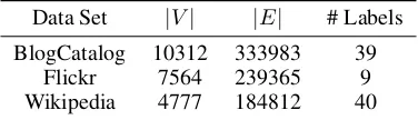
Table 1: Data sets for experiments Data Set |V| |E| # Labels BlogCatalog 10312 333983 39

Flickr 7564 239365 9

Wikipedia 4777 184812 40

of a normal prior over the embedding vector while the part of (6) related to sampling can be viewed as the log likelihood of the model. Therefore the whole objective of R-NS can be regarded as the logarithm of the posterior distribution of the embedding vectors given the network. The inclusion of the prior allows the method to borrow information from other nodes to estimate the embedding vector for a particular node. The experiment section also shows the importance of norm penalization. Regarding the choice of`2norm over`1norm,

we tried both norms in the process of coming up with R-NS. In many cases`2performed better and we did not have a

mo-tivation for the sparsity of the embedding vectors. Therefore we used`2norm penalization.

Scalability The R-NS objective has a different negative sampling distribution for different nodes, so we need a method to draw negative samples from the desired distri-bution without changing the time complexity. We suggest two methods for adaptive sampling, depending on whether the network is densely connected or not. The details of the two suggested methods are presented in the supplementary material.

Experiments

In this section we show the superiority of R-NS to NS for multi-label classification tasks on several large-scale net-works. We also illustrate in the appendix the undesirable effects of the popular neighbor problem on the embedding vectors through the analysis of a small real network and we show how R-NS alleviates the problem.

(6)

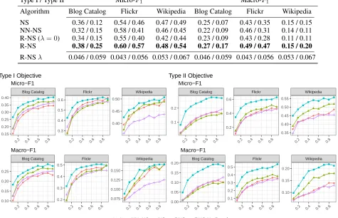
Table 2: Algorithm comparison for 50% data labeled, Type I and II objectives. The maximum standard deviation of the presented numbers for type I and type II are respectively 0.005 and 0.0072. The exact standard deviation of the methods and ROC curves can be found in the supplementary file.

Type I / Type II Micro-F1 Macro-F1

Algorithm Blog Catalog Flickr Wikipedia Blog Catalog Flickr Wikipedia NS 0.36 / 0.12 0.54 / 0.46 0.47 / 0.49 0.25 / 0.07 0.43 / 0.35 0.15 / 0.15 NN-NS 0.32 / 0.15 0.58 / 0.41 0.46 / 0.45 0.22 / 0.09 0.46 / 0.31 0.14 / 0.11 R-NS (λ= 0) 0.34 / 0.15 0.55 / 0.40 0.42 / 0.44 0.23 / 0.09 0.43 / 0.28 0.11 / 0.11 R-NS 0.38 / 0.25 0.60 / 0.57 0.48 / 0.54 0.27 / 0.17 0.49 / 0.47 0.15 / 0.20 R-NSλ 0.046 / 0.059 0.043 / 0.056 0.053 / 0.067 0.046 / 0.059 0.043 / 0.056 0.053 / 0.067

Type I Objective Type II Objective

Blog Catalog Flickr Wikipedia

0.2 0.4 0.6 0.8 0.2 0.4 0.6 0.8 0.2 0.4 0.6 0.8 0.40

0.45 0.50

0.3 0.4 0.5 0.6

0.15 0.20 0.25 0.30 0.35 0.40

Micro−F1

0.2 0.4 0.6 0.8 0.2 0.4 0.6 0.8 0.2 0.4 0.6 0.8 0.35

0.40 0.45 0.50 0.55

0.2 0.4 0.6

0.1 0.2

Micro−F1

0.2 0.4 0.6 0.8 0.2 0.4 0.6 0.8 0.2 0.4 0.6 0.8 0.075

0.100 0.125 0.150

0.2 0.3 0.4 0.5

0.10 0.15 0.20 0.25

Macro−F1

0.2 0.4 0.6 0.8 0.2 0.4 0.6 0.8 0.2 0.4 0.6 0.8 0.10

0.15 0.20

0.1 0.2 0.3 0.4 0.5

0.00 0.05 0.10 0.15 0.20

Macro−F1

Method NN−NS NS RNS RNS No Penalty

Figure 1: Multi-label classification performance comparison on the datasets with varying amounts of labeled training data, averaged over 5 iterations. Thexaxis is the fraction of data with labels, the y axis is theF1score. For both types of objective

RNS leads to improved performance.

Multi-label classification

The multi-label classification task entails predicting the pos-sibly multiple labels associated with each node in the given network. A fraction of nodes and their labels are observed. This training set information is used to predict the labels of the nodes in the test set, the remaining nodes. This is a common task for evaluating network embeddings (Huang et al. 2018).

Data Sets We use the following datasets. The BlogCatalog dataset (Zafarani and Liu 2009) is a friendship network of bloggers on the BlogCatalog website. The labels are cate-gories which the bloggers use to tag their posts. The Flickr dataset (Huang, Li, and Hu 2017a) is a network of interactions between Flickr users. The labels represent the interest groups of the users such as “black and white photos”. The Wikipedia dataset (Mahoney 2011) is the word co-occurrence network of the Wikipedia dataset, which used a 2-word window to determine co-occurrence edges. They used the Stanford

POS-Tagger to infer parts of speech for words in the network, and treat these as the labels.

Compared Algorithms. To validate the performance of our approach we compare R-NS with NS and several alterna-tives to R-NS that also can scale up to large networks.

• Non-neighbor Negative Sampling (NN-NS). This algo-rithm differs from the R-NS procedure explained in the previous section in the negative sampling distributionPu,

where a node also can chose itself as a negative sample. To be more specific,Puself sample(v)∝dvβforv ∈V −N(u)

but the probability of choosingv∈N(u)is zero. One can show that self negative sampling in the type I objective case is equivalent to having a penalty on the norm.

• R-NS (no penalty). This algorithm is different form R-NS in that it does not penalize the norms of the embedding vectors which is equivalent toλ= 0.

(7)

pre-vious section which optimizes the objective that is the summation of terms like (6) for all pairs of a node and its neighbor.

Given the empirical results in both natural language pro-cessing and network embedding demonstrating the superior-ity of NS versus competing methods (Mikolov et al. 2013b), we did not include direct optimization of SGA objective, noise contrastive estimation, nor hierarchical softmax in the baseline methods.

Parameter settings mostly follow previous literature. The penalty coefficientλis calculated based on the formula given in the paper. The degree powerβis chosen to be3/4, which is a widespread default in the literature. Exact settings are presented in the supplementary file.

Experimental Results The network embeddings are used in a one-vs-all logistic regression with L2 penalty, imple-mented through the LibLinear library. From Table 2, we see that simply excluding neighbors from negative sampling is insufficient, as R-NS(no penalty) underperforms even the standard negative sampling scheme. This also demonstrates the importance of the norm penalization. NN-NS is presented to show the importance of deriving a formula for the penalty coefficient. NN-NS can be perceived as R-NS with a penalty coefficient on the norm where the penalty depends on the degree of the node. This is the case because NN-NS, like R-NS, does not let negative samples be from the neighbors. And since it lets a node choose itself as a negative sample with probability related to the degree, it can be considered to do degree-related norm penalization. NN-NS does not have enough freedom on the form of the penalty, unlike R-NS, and that can be seen as the main reason that it does not perform as well as R-NS. See Table 2 for a comparison of the algorithms. To provide further intuition about the performance of the methods, we conduct experiments where we randomly divide the data into train and test splits and increase the proportion of training examples from 10% to 90% of the data in increments of 10%. The results for each dataset, averaged over multiple iterations, are summarized in Figure 1. We see that R-NS leads to a significant improvement over NS in both multi-label Micro-F1and Macro-F1scores for embeddings using

both the Type I and Type II objectives for most train-test splits. It also improves on NN-NS and R-NS (no penalty). For most of the experimental set ups NN-NS and R-NS with no penalty do not provide much improvement over NS and in fact underperform NS for Type I and Type II embeddings on the Blog Catalog and Wikipedia datasets. In particular for the Blog Catalog network with Type II embeddings, R-NS outperforms R-NS in terms of Micro-F1 score by about

94% for 50% of the training data labeled. Meanwhile for the Flickr data with Type II embeddings R-NS outperforms NS in terms of Micro-F1score by about 126% for only 10% of

the training data labeled.

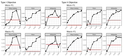
To see the importance of choosing a properλ, and to gain a general intuition for howλeffects the quality of the em-beddings, we also vary theλin R-NS and compare the result with NS. We clarify again that the result of the experiments in Table 2 and Figure 1 are based on the formula which is

Type I Objective Type II Objective

0.00 0.02 0.04 0.06 0.00 0.02 0.04 0.06 0.00 0.02 0.04 0.06

0.46 0.47 0.48 0.49

0.54 0.56 0.58 0.60

0.33 0.34 0.35 0.36 0.37 0.38

Micro−F1

0.00 0.02 0.04 0.06 0.00 0.02 0.04 0.06 0.00 0.02 0.04 0.06

0.48 0.50 0.52 0.54

0.48 0.52 0.56

0.125 0.150 0.175 0.200 0.225 0.250

Micro−F1

0.00 0.02 0.04 0.06 0.00 0.02 0.04 0.06 0.00 0.02 0.04 0.06

0.14 0.15 0.16

0.44 0.46 0.48 0.50

0.23 0.24 0.25 0.26

Macro−F1

0.00 0.02 0.04 0.06 0.00 0.02 0.04 0.06 0.00 0.02 0.04 0.06

0.14 0.16 0.18 0.20

0.35 0.40 0.45

0.075 0.100 0.125 0.150 0.175

Macro−F1

Figure 2: Effect of penaltyλon multi-label classification per-formance for data with 50% of labels withheld, averaged over 5 iterations. The red Horizontal line indicates performance of NS.

given in the paper, not by searching over the grids of theλ. Figure 2 shows the effect of different λsettings on F1

scores when the train-test split is set to 50%, averaged over 5 iterations. Note that especially in the case of the Blog Catalog and Wikipedia Network datasetsλshould be within a suitable region in order for R-NS to outperform NS. Since in all of the experimental results R-NS is superior to NS when it uses the presented formulation forλ, the formula assigns a suitable value toλbased on the network.

Source code for running experiments and data are available online at https://github.com/delimited0/network embedding.

Conclusion

In this paper we examined the performance of the NS ap-proximation to the SGA objective for network embedding. We showed NS suffers from the Popular Neighbor Problem, which can lead to embedding vectors with undesirable prop-erties that are contrary to the goals of the SGA objective and network embedding.We proposed R-NS, which avoids the Popular Neighbor Problem. We demonstrated the efficiency and effectiveness of R-NS by doing experiments on several real-world networks. Moreover, because of the careful design of R-NS, the method is scalable and can be employed for the learning of embeddings in an unsupervised fashion.

For future work we plan to apply R-NS to other areas where NS is widely used, such as natural language processing, and evaluate its performance. We also plan to investigate more intelligent schemes for choosing negative samples that use more information than just the degree of a node and the set of its neighbors. For example we could consider the structure of the nodes and its measure of connectivity when taking negative samples.

Acknowledgments

We thank the anonymous reviewers for their feedback. This work is, in part, supported by NSF (1750074 and #IIS-1718840).

References

Bhagat, S.; Cormode, G.; and Muthukrishnan, S. 2011. Node

(8)

Cao, S.; Lu, W.; and Xu, Q. 2016. Deep neural networks for

learning graph representations. InAAAI, 1145–1152.

Chen, L.; Yuan, F.; Jose, J. M.; and Zhang, W. 2018. Improving negative sampling for word representation using self-embedded

features. InProceedings of the Eleventh ACM International

Con-ference on Web Search and Data Mining, 99–107. ACM. Cui, P.; Wang, X.; Pei, J.; and Zhu, W. 2018. A survey on

net-work embedding. IEEE Transactions on Knowledge and Data

Engineering.

Friedman, J.; Hastie, T.; and Tibshirani, R. 2001. The elements

of statistical learning, volume 1. Springer series in statistics New York, NY, USA:.

Grover, A., and Leskovec, J. 2016. Node2vec: Scalable

fea-ture learning for networks. InProceedings of the 22Nd ACM

SIGKDD International Conference on Knowledge Discovery and Data Mining, KDD ’16.

Gutmann, M. U., and Hyv¨arinen, A. 2012. Noise-contrastive es-timation of unnormalized statistical models, with applications to

natural image statistics. Journal of Machine Learning Research

13(Feb):307–361.

Huang, X.; Song, Q.; Li, J.; and Hu, X. 2018. Exploring expert

cognition for attributed network embedding. InACM

Interna-tional Conference on Web Search and Data Mining, 270–278. Huang, X.; Li, J.; and Hu, X. 2017a. Accelerated attributed

net-work embedding. InProceedings of the 2017 SIAM International

Conference on Data Mining, 633–641. SIAM.

Huang, X.; Li, J.; and Hu, X. 2017b. Label informed attributed

network embedding. InACM International Conference on Web

Search and Data Mining, 731–739.

Lai, Y.; Hsu, C.; Chen, W.; Yeh, M.; and Lin, S. 2017. PRUNE: preserving proximity and global ranking for network embedding.

InNIPS, 5263–5272.

Liben-Nowell, D., and Kleinberg, J. 2003. The link prediction

problem for social networks. InProceedings of the Twelfth

In-ternational Conference on Information and Knowledge

Manage-ment, CIKM ’03.

Maaten, L. v. d., and Hinton, G. 2008. Visualizing data using

t-sne.Journal of machine learning research9(Nov):2579–2605.

Mahoney, M. 2011. Large text compression benchmark. Mikolov, T.; Chen, K.; Corrado, G. S.; and Dean, J. 2013a.

Effi-cient estimation of word representations in vector space. CoRR

abs/1301.3781.

Mikolov, T.; Sutskever, I.; Chen, K.; Corrado, G.; and Dean, J. 2013b. Distributed representations of words and phrases and

their compositionality. InProceedings of the 26th International

Conference on Neural Information Processing Systems - Volume

2, NIPS’13, 3111–3119. USA: Curran Associates Inc.

Mnih, A., and Teh, Y. W. 2012. A fast and simple algorithm

for training neural probabilistic language models.arXiv preprint

arXiv:1206.6426.

Morin, F., and Bengio, Y. 2005. Hierarchical probabilistic neural network language model. volume 5, 246–252. Citeseer.

Mu, C.; Yang, G.; and Yan, Z. 2018. Revisiting skip-gram

negative sampling model with regularization. arXiv preprint

arXiv:1804.00306.

Perozzi, B.; Al-Rfou, R.; and Skiena, S. 2014. Deepwalk:

On-line learning of social representations. InProceedings of the 20th

ACM SIGKDD International Conference on Knowledge Discov-ery and Data Mining, KDD ’14, 701–710.

Ribeiro, L. F.; Saverese, P. H.; and Figueiredo, D. R. 2017.

Struc2vec: Learning node representations from structural

iden-tity. InProceedings of the 23rd ACM SIGKDD International

Conference on Knowledge Discovery and Data Mining, KDD ’17.

Sadeghian, A.; Rodriguez, M.; Wang, D. Z.; and Colas, A. 2016. Temporal reasoning over event knowledge graphs.

Shaw, B., and Jebara, T. 2009. Structure preserving embedding. InProceedings of the 26th Annual International Conference on Machine Learning, ICML ’09, 937–944. New York, NY, USA: ACM.

Tang, J.; Qu, M.; Wang, M.; Zhang, M.; Yan, J.; and Mei, Q. 2015. Line: Large-scale information network embedding. In

Proceedings of the 24th International Conference on World Wide

Web, WWW ’15, 1067–1077.

Tu, C.; Zhang, W.; Liu, Z.; Sun, M.; et al. 2016. Max-margin deepwalk: Discriminative learning of network representation. In

IJCAI, 3889–3895.

Tu, K.; Cui, P.; Wang, X.; Yu, P. S.; and Zhu, W. 2018. Deep

recursive network embedding with regular equivalence. In

Pro-ceedings of the 24th ACM SIGKDD International Conference on Knowledge Discovery & Data Mining, 2357–2366. ACM. Wang, X.; Cui, P.; Wang, J.; Pei, J.; Zhu, W.; and Yang, S. 2017.

Community preserving network embedding. InAAAI, 203–209.

Yang, Z.; Cohen, W. W.; and Salakhutdinov, R. 2016.

Revis-iting semi-supervised learning with graph embeddings. In

Pro-ceedings of the 33rd International Conference on International Conference on Machine Learning - Volume 48, ICML’16, 40–48. JMLR.org.

Zachary, W. 1977. An information flow model for conflict and

fission in small groups. J. of Anthropological Research33:452–

473.

Zafarani, R., and Liu, H. 2009. Social computing data repository at ASU.

Zhang, Z.; Cui, P.; Wang, X.; Pei, J.; Yao, X.; and Zhu, W. 2018.

Arbitrary-order proximity preserved network embedding. In