Knowledge Transfer via Distillation of Activation Boundaries Formed by Hidden Neurons

The Thirty-Third AAAI Conference on Artificial Intelligence (AAAI-19)

Knowledge Transfer via Distillation of

Activation Boundaries Formed by Hidden Neurons

Byeongho Heo,

Minsik Lee,

Sangdoo Yun,

Jin Young Choi

1_{Department of ECE, ASRI, Seoul National University, Korea}

2_{Division of EE, Hanyang University, Korea} 3_{Clova AI Research, NAVER Corp, Korea}

Abstract

An activation boundary for a neuron refers to a separating hyperplane that determines whether the neuron is activated or deactivated. It has been long considered in neural networks that the activations of neurons, rather than their exact output values, play the most important role in forming classification-friendly partitions of the hidden feature space. However, as far as we know, this aspect of neural networks has not been considered in the literature of knowledge transfer. In this pa-per, we propose a knowledge transfer method via distillation of activation boundaries formed by hidden neurons. For the distillation, we propose an activation transfer loss that has the minimum value when the boundaries generated by the stu-dent coincide with those by the teacher. Since the activation transfer loss is not differentiable, we design a piecewise dif-ferentiable loss approximating the activation transfer loss. By the proposed method, the student learns a separating bound-ary between activation region and deactivation region formed by each neuron in the teacher. Through the experiments in various aspects of knowledge transfer, it is verified that the proposed method outperforms the current state-of-the-art.

Introduction

Learning deep neural networks requires much time and com-putational resource. Many studies have been conducted to make the learning process lighter and faster, one of which is to transfer knowledge. Knowledge transfer is to accelerate and improve learning of a new network (student) by transfer-ring knowledge from a previously learned network (teacher). If the network architectures are identical, knowledge trans-fer can be simply conducted by copying the parameters from teacher to student. However, in general, knowledge transfer aim to improve the performance of a small network (student) based on a large network (teacher). Knowledge transfer be-tween different network architectures is a challenging prob-lem and has not been completely solved.

The main direction of knowledge transfer is to transfer neuron responses of hidden layers. Romero et al. (2015) pro-posed a knowledge transfer method based on hidden layer responses. Zagoruyko and Komodakis (2017) changed the form of hidden neuron responses to an attention map, while Yim et al. (2017) used the form of Gram matrix (Gatys,

Copyright c2019, Association for the Advancement of Artificial Intelligence (www.aaai.org). All rights reserved.

Ecker, and Bethge 2016). The hidden layers of a neural net-work contains a lot of information and is suitable for knowl-edge transfer. However, due to the high dimensionality and non-linearity of the hidden layer neurons, it is not easy to achieve a perfect transfer.

The activation boundary is a separating hyperplane that determines whether neurons are active or deactivated. In neural networks, the activation of neurons has been con-sidered to be important for a long time. Recently, regard-ing the activation boundary, Montufar et al. (2014) and Pas-canu, Mont´ufar, and Bengio (2014) reported that a neural network expresses a complex function with a combination of activation boundaries. Pan and Srikumar (2016) provided the fact that the decision boundary of a neural network is composed of a combination of activation boundaries. These studies give an insight that the transfer of activation bound-ary information in the teacher to the student could greatly contribute to an improvement of knowledge transfer perfor-mance in classification problems, because a classification problem highly depends on the formation of decision bound-aries among classes.

learn-ing and compare the proposed method in more general case. Finally, the proposed method is analyzed through several ex-periments.

Related Work

Rectified Linear Unit (ReLU) (Nair and Hinton 2010) ac-tivation, which is less affected by the vanishing gradient problem, has become the basis of various network archi-tectures (Krizhevsky, Sutskever, and Hinton 2012; Szegedy et al. 2015; He et al. 2016). At the same time, studies on ReLU-based networks have been conducted. ReLU activa-tion divides the input space into two, and the dividing hy-perplane between the two is called the activation bound-ary. Activation boundaries of multiple neurons divide the input space several times. Thus, the function expressed by the neural network is a set of piecewise linear partitions that are divided by the activation boundaries. This is the appear-ance of a ReLU-based network that is commonly described in studies. (Montufar et al. 2014; Pascanu, Mont´ufar, and Bengio 2014; Pan and Srikumar 2016). Based on this piece-wise linear partitions, Montufar et al. (2014) and Pascanu, Mont´ufar, and Bengio (2014) propose to use the number of partitions divided by the activation boundaries as a measure of complexity of a network. In other words, the complex-ity of a neural network depends on the placement of ac-tivation boundaries. Pan and Srikumar (2016) shows that the binary decision of a ReLU-based network is the same as the combination of threshold functions at the activation boundaries. This means that the knowledge of a ReLU-based network is concentrated at the activation boundaries. These studies imply that an activation boundary is a key factor of ReLU-based networks. Despite such importance of activa-tion boundaries, convenactiva-tional knowledge transfer methods, as far as we know, do not aim to transfer activation bound-aries.

Romero et al. (2015) first proposed a method of transfer-ring the neuron responses of hidden layers for knowledge distillation. In this method, the entire neurons in hidden lay-ers were transferred using the mean square error function. This approach was effective for the high-level hidden lay-ers but not for the low-level hidden laylay-ers. Subsequent stud-ies have attempted to reduce the dimension of neurons to cope with low-level hidden layers. In a convolutional neu-ral network, the hidden layer response is a tensor consisting of two spatial dimensions and one channel dimension. Yim et al. (2017) focus on channel dimensions and reduce spatial information. In this work, only correlation between channels is transferred using a method similar to Gram matrix (Gatys, Ecker, and Bethge 2016). Conversely, Zagoruyko and Ko-modakis (2017) concentrates on spatial attention and re-duces channel information. Neuron responses are averaged over the channel and only spatial information is transferred. Both method succeed in transferring low-level hidden lay-ers, however, both channel and spatial information are im-portant information, and reducing dimension is a loss of information. If low-level hidden layers can be transferred without dimension reduction, the performance of knowl-edge transfer might be improved. Therefore, using activa-tion boundaries, we challenge to transfer the entire neuron

responses without reducing dimension.

Method

There are two types of learning schemes for transferring the responses of the hidden layer neurons from a teacher net-work to a student netnet-work. The first approach transfers the neuron responses during the student neural network learns to classify input images (Zagoruyko and Komodakis 2017; Srinivas and Fleuret 2018; Hinton, Vinyals, and Dean 2015). In this case, the cross entropy loss and the transfer loss are combined to form a single integrated loss which is used for the whole training process. The second approach is to transfer the neuron responses for initializing the student net-work before the classification training (Romero et al. 2015; Yim et al. 2017). After the network is initialized based on the transfer loss, it is trained for classification based on the cross-entropy loss. In this paper, we discuss knowledge transfer based on the second approach, which is the network initialization method, to analyze the transfer loss indepen-dently.

A part of the teacher network, the part from the input im-age to a hidden layer, is defined as a functionT, and a part of the student network is defined as a function S. For an imageI, the neuron response vector of the hidden layer is T(I)∈RMfor the teacher andS(I)∈RM for the student.

M is the number of neurons in the hidden layer. For con-venience, we assume that the teacher and the student have hidden layers of the same size. In order to describe the ac-tivation of neurons,T(I)andS(I)are defined as the val-ues before the activation functions. Here, we consider the element-wise ReLU σ(x) = max(0, x) as the activation function.

An existing method (Romero et al. 2015) of neuron re-sponse transfer is as follows.

L(I) =kσ(T(I))−σ(S(I))k2₂ (1)

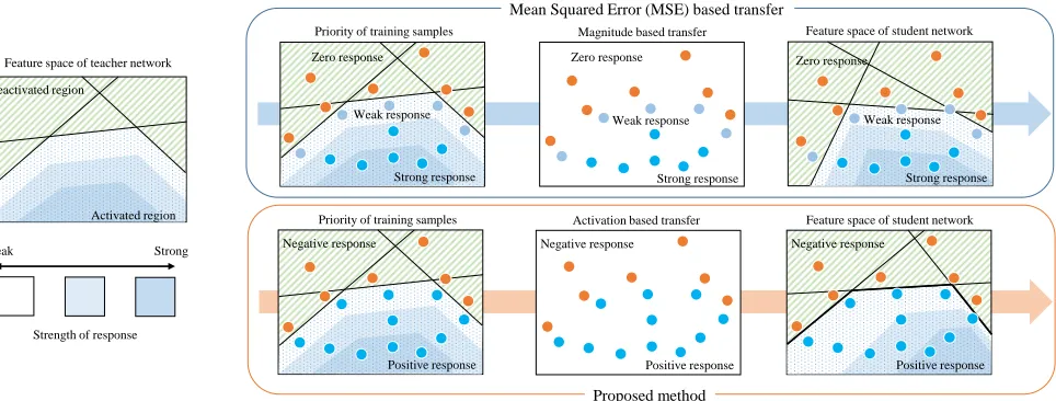
It is the mean square error function between neuron re-sponses after the ReLU activation. (1) makes a student merely approximate the neuron responses of the teacher, but the resulting activation boundaries can be wildly dif-ferent. Figure 1 shows an example. The mean square error is a loss that is biased to a large difference, so this will mainly transfer samples with strong responses. However, as shown in Figure 1, the activation boundaries are between weak responses and zero responses. The mean square error can hardly distinguish between weak responses and zero re-sponses, so it is difficult to transfer the activation boundaries by the method based on ( 1).

Weak response Zero response

Priority of training samples

Priority of training samples

Negative response

Strong response Magnitude based transfer

Weak response Zero response

Activation based transfer

Positive response Negative response

Feature space of student network

Zero response

Feature space of student network

Negative response

Mean Squared Error (MSE) based transfer

Proposed method

Positive response

Strong response Strong response

Weak response

Positive response Deactivated region

Feature space of teacher network

Activated region

Strength of response Strong Weak

Figure 1: The concept of the proposed knowledge transfer method. The proposed method concentrates on the activation of neurons, not the magnitude of neuron responses. This concentration enables more precise transfer of the activation boundaries.

whether a neuron is activated or not, i.e.,

ρ(x) =

1, ifx >0

0, otherwise. (2)

The new loss to transfer the neuron activation is given by

L(I) =kρ(T(I))−ρ(S(I))k₁, (3)

which is referred to as the activation transfer loss in our paper. The activation transfer loss is a function that gives a constant penalty when the activations of teacher and stu-dent are different. Regardless of the magnitude of neuron responses, all neurons have the same weight. The lower part of Figure 1 shows knowledge transfer using the activation transfer loss. Although the magnitude of neuron responses are not well transferred, it is trained to keep the activation of teacher neurons. Thus, the activation boundaries are accu-rately transferred. Considering the importance of activation boundaries in a neural network, the activation transfer loss is more efficient in knowledge transfer than the mean square error.

The activation transfer loss is suitable for transfer of acti-vation boundaries. However, sinceρ()is a discrete function, the activation transfer loss can not be minimized by gradient descent. Therefore, we propose an alternative loss that can be minimized by gradient descent. Minimizing the activation transfer loss is similar to learning a binary classifier. The ac-tivation of teacher neuronsρ(T(I))correspond to class la-bels. The response of student neuron should be greater than 0 if the teacher neuron is active and less than 0 if the teacher neuron is deactivated. Inspired by this similarity, the alterna-tive loss is designed similar to the hinge loss (Rosasco et al. 2004) used in SVM (Cortes and Vapnik 1995).

L(I) =kρ(T(I))σ(µ1− S(I))

+ (1−ρ(T(I)))σ(µ1+S(I))k2₂ (4)

The symbolmeans element-wise product of vectors. The

1represents a vector of lengthM where all component val-ues are equal to one. The alternative loss gives a square penalty for student neurons with different activations, and does not care about neurons with the same activation. In addition, the margin µ is introduced for stability of train-ing. To understand the alternative loss function, we explain it in terms of gradients. For convenience, the i-th element of neuron response vector is denoted asti (teacher) andsi

(student). The derivative of (4) with respect tosiis

−∂L(I) ∂si

=

 



2(si−µ), ifρ(ti) = 1andsi< µ

−2(si+µ), ifρ(ti) = 0andsi>−µ

0, otherwise.

(5) When the teacher neuron is activated and the student re-sponse is less than a marginµ, then the gradient becomes positive. Conversely, when the teacher neuron is deactivated and the student response is greater than the minus margin −µ, the gradient becomes negative. Otherwise, the gradi-ent is zero. Therefore, minimizing the alternative loss makes neurons of the teacher and student have the same activation, and puts a margin to the student’s neuron response for sta-bility. The proposed method is to transfer neuron responses using the alternative loss. Since the alternative loss approx-imates the activation transfer loss, the proposed method transfers the activation boundaries. Effectiveness of the pro-posed method and the fact that the alternative loss actually approximates the activation transfer loss are verified in the experiment section.

Number of neurons

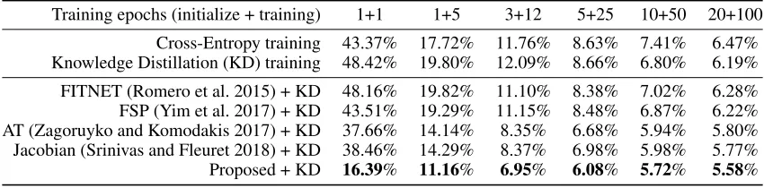
Table 1: Learning speed experiment using various training epochs. Table shows error rate(%) on test set.

Training epochs (initialize + training) 1+1 1+5 3+12 5+25 10+50 20+100

Cross-Entropy training 43.37% 17.72% 11.76% 8.63% 7.41% 6.47% Knowledge Distillation (KD) training 48.42% 19.80% 12.09% 8.66% 6.80% 6.19%

FITNET (Romero et al. 2015) + KD 48.16% 19.82% 11.10% 8.38% 7.02% 6.28% FSP (Yim et al. 2017) + KD 43.51% 19.29% 11.15% 8.48% 6.87% 6.22% AT (Zagoruyko and Komodakis 2017) + KD 37.66% 14.14% 8.35% 6.68% 5.94% 5.80% Jacobian (Srinivas and Fleuret 2018) + KD 38.46% 14.29% 8.37% 6.98% 5.98% 5.77% Proposed + KD 16.39% 11.16% 6.95% 6.08% 5.72% 5.58%

of neurons might be different. In this case, we use a con-nector function that consists of simple operations (Romero et al. 2015). Let the number of neurons in a teacher net-work beM (T(I)∈_RM_{), and the number of neurons in a}

student networkN (S(I) ∈ RN). The connector function

r:_RN _→

RM converts a neuron response vector of student

to the size of teacher vector. Using the connector function, the alternative loss (4) is changed as

L(I) =kρ(T(I))σ(µ1−r(S(I)))

+ (1−ρ(T(I)))σ(µ1+r(S(I)))k2₂. (6)

Typically, the connector function is a fully connected layer or a combination of a fully connected layer and a batch nor-malization layer. In the initialization process, the connector functionr and the student networkS are trained simulta-neously to minimize (6). After the initialization for knowl-edge transfer, only the student network without the connec-tor function is used for classification. Romero et al. first pro-pose the use of connector functions in knowledge transfer. It is based on an idea that if a student can represent a teacher with a simple converting operation, the student has the same level of knowledge as the teacher. The connector function is effectively applied to knowledge transfer and allows the proposed method to be applied even when the number of neurons is different.

Convolutional neural network

Convolutional neural networks take an image as input and create hidden neuron responses with spatial dimensions. Let the number of hidden neurons beH×W×M(height, width, channel). Since a convolutional operation shares weights for each spatial location,H ×W ×M neuron responses can be interpreted as an M dimensional neuron response for H ×W receptive fields on an image (Lecun et al. 1998; Long, Shelhamer, and Darrell 2015). Therefore, the pro-posed method can be applied to each spatial location of the neuron responses. For a neuron response tensor T(I) ∈

RH×W×M andS(I)∈RH×W×N, let the neuron response

vector at the (i, j)-th spatial position beT(I)ij ∈ RM and

S(I)ij∈RN,(i= 1,· · ·, H;j = 1,· · ·, W), respectively.

The proposed loss is represented as a sum over spatial

loca-tions.

L(I) = H

X

i W

X

j

kρ(T(I)ij)σ(µ1−r(S(I)ij))

+ (1−ρ(T(I)ij))σ(µ1+r(S(I)ij))k

2 2. (7)

Using (7), the proposed method can also be applied to a con-volutional neural network. In this case, the connector func-tion ris shared at all spatial locations, so a 1×1 convolu-tional layer is used instead of a fully connected layer. In this case, teacher and student layers are forced to be of the same spatial size. Therefore, like other knowledge transfer meth-ods (Romero et al. 2015; Zagoruyko and Komodakis 2017; Srinivas and Fleuret 2018), a hidden layer which has the same spatial size as that of the teacher is selected for the target of knowledge transfer.

Experiments

We verified the proposed method through various exper-iments. The first experiment is about various aspects of knowledge transfer. Experiments that can verify the benefits of knowledge transfer are designed. Through experiments, we show that the proposed method outperforms the current state-of-the-art in most aspects. For the next experiment, we evaluated the proposed method in transfer learning to ver-ify its performance in more general configurations. In trans-fer learning, using a teacher pre-trained on ImageNet (Rus-sakovsky et al. 2015), a randomly initialized student was trained on a target dataset other than ImageNet. We mea-sured performance on the scene classification dataset (Quat-toni and Torralba 2009) and the fine-grained bird classifica-tion dataset (Wah et al. 2011) that have different properties from ImageNet. Finally, several analytical experiments were conducted to help understand the proposed method.

Knowledge transfer for the same task

Table 2: Performance for small size training data. Table shows error rate (%) on test set.

Percentage of training data 0.1% 1% 5% 10% 20% 100%

Cross-Entropy training 73.83% 48.41% 28.12% 21.76% 15.26% 6.47% Knowledge Distillation (KD) training 74.62% 48.34% 28.13% 21.21% 14.62% 6.19%

FITNET (Romero et al. 2015) + KD 74.81% 49.91% 27.28% 21.42% 14.52% 6.28% FSP (Yim et al. 2017) + KD 73.96% 47.98% 26.90% 20.80% 13.85% 6.22% AT (Zagoruyko and Komodakis 2017) + KD 67.54% 37.11% 18.86% 15.61% 9.94% 5.80% Jacobian (Srinivas and Fleuret 2018) + KD 68.65% 36.99% 18.34% 15.03% 9.83% 5.77% Proposed + KD 50.32% 21.54% 14.99% 13.09% 9.16% 5.58%

Table 3: Performance for various sizes of networks. Table shows error rate(%) on test set.

Compression type Teacher Student Size ratio KD FITNET FSP AT Jacobian Proposed

Depth WRN 22-4 WRN 10-4 27.9% 22.98% 23.34% 22.99% 18.06% 18.28% 14.05% Channel WRN 16-4 WRN 16-2 25.2% 20.48% 19.98% 19.78% 14.81% 14.41% 11.62% Depth & Channel WRN 22-4 WRN 16-2 16.1% 21.21% 21.42% 20.80% 15.61% 15.03% 13.09% Tiny network WRN 22-4 WRN 10-1 1.8% 29.57% 29.18% 28.70% 29.44% 28.70% 23.27% Same network WRN 16-4 WRN 16-4 100% 18.29% 17.91% 17.81% 12.03% 11.28% 6.63%

and is using 4 times the number of base channels. As base-line, we used the Knowledge Distillation (KD) loss (Hin-ton, Vinyals, and Dean 2015) which is commonly used for knowledge transfer in the same dataset. We have also pre-sented the training result without any knowledge transfer. The compared algorithms were implemented based on the author-provided codes and the papers. Details on implemen-tation are discussed in the last subsection.

First, we compared the algorithms in terms of learning speed. Since knowledge transfer uses information of a pre-trained network, it can accelerate the training of a new net-work. The learning speed was measured in terms of clas-sification performance on various training epochs. Experi-ments were conducted with WRN22-4 as a teacher network and WRN16-2 as a student network. In this case, the error rate of the teacher is 4.51%. Table 1 shows the results. The top row of Table 1 indicates the numbers of epochs used for network initialization and classification training. The rest of the rows represent the classification error (%) of the student network on the test set. Most knowledge transfer algorithms accelerate the learning of the student network. Therefore, as the training epoch decreases, their relative performance improvement increases. Here, we can confirm that the pro-posed method outperforms other algorithms in all cases. In particular, the performance gap becomes larger as the train-ing epochs becomes shorter. Therefore, the proposed method is superior to the current state-of-the-art in terms of learning speed.

The second experiment is about small training data. When the size of training data is small, it is difficult to achieve good generalization performance. If there is a teacher net-work with a good generalization performance, knowledge transfer can help the student network to improve its general-ization performance. In order to test this property, we mea-sured the performance when the training data was limited to a certain ratio. As in the previous experiment, WRN22-4

and WRN16-2 were used as the teacher and the student, re-spectively. The teacher network was trained using the whole training data, and the error rate was 4.51%. For training the student network, if the ratio of training data was more than 10%, the number of training epochs was fixed to 120 epochs. If the ratio was less than 10%, we increased the number of epochs to maintain a certain amount of training iterations. 240 epochs were used for 5%, 1,200 epochs for 1%, and 12,000 epochs were used for 0.1%. The results are shown in Table 2. Most knowledge transfer methods help the stu-dent classifier generalize well, and the smaller the learning data, the greater the performance improvement by knowl-edge transfer. Again in this case, the proposed method shows the best performance for all scenarios. Especially, the pro-posed method is more effective when there is little training data. Therefore, the proposed method can be the most effec-tive choice for a small amount of training data.

The last experiment is about knowledge transfer for net-works of various sizes. One of the main uses of knowledge transfer is for network compression and it has the advan-tage of being able to cope with various network sizes. In this experiment, we measured the performance of knowl-edge transfer for various configurations of network sizes. In this experiment, training was performed for 120 epochs us-ing 10% of the trainus-ing data. The experimental results are shown in Table 3. Here, we can see that all knowledge trans-fer algorithms, including the proposed method, are more vulnerable to depth compression than to channel compres-sion. However, the proposed method still achieves the best performance for all cases. In particular, in case of “Tiny net-work”, the proposed method greatly increases performance from the baseline, while the other methods have little im-provement. Therefore, the proposed method is better solu-tion for the various type of network compression than other methods.

Table 4: Performance of transfer learning on MIT scenes. Table shows accuracy (%) on test set.

Number of training data per class 5 10 20 40 80

ImageNet pre-trained network 32.39% 42.46% 52.99% 62.54% 69.78%

randomly initialized network 11.12% 17.99% 30.37% 43.88% 56.94% DTL on randomly initialized network 20.52% 34.55% 49.78% 59.48% 64.93%

FITNET (Romero et al. 2015) + DTL 29.55% 43.81% 53.51% 63.36% 66.57% FSP (Yim et al. 2017) + DTL 25.60% 39.63% 51.42% 60.08% 63.73% AT (Zagoruyko and Komodakis 2017) + DTL 22.61% 35.37% 49.10% 60.15% 65.15% Jacobian (Srinivas and Fleuret 2018) + DTL 26.64% 38.28% 51.34% 61.19% 63.96% Proposed + DTL 43.36% 56.72% 66.34% 70.75% 74.10%

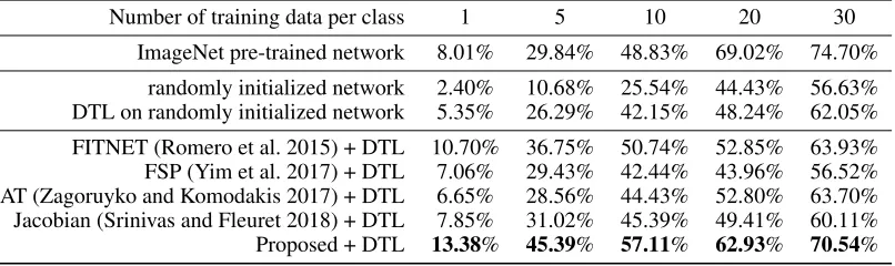
Table 5: Performance of transfer learning on CUB 2011 dataset. Table shows accuracy (%) on test set.

Number of training data per class 1 5 10 20 30

ImageNet pre-trained network 8.01% 29.84% 48.83% 69.02% 74.70%

randomly initialized network 2.40% 10.68% 25.54% 44.43% 56.63% DTL on randomly initialized network 5.35% 26.29% 42.15% 48.24% 62.05%

FITNET (Romero et al. 2015) + DTL 10.70% 36.75% 50.74% 52.85% 63.93% FSP (Yim et al. 2017) + DTL 7.06% 29.43% 42.44% 43.96% 56.52% AT (Zagoruyko and Komodakis 2017) + DTL 6.65% 28.56% 44.43% 52.80% 63.70% Jacobian (Srinivas and Fleuret 2018) + DTL 7.85% 31.02% 45.39% 49.41% 60.11% Proposed + DTL 13.38% 45.39% 57.11% 62.93% 70.54%

proposed method in various configurations of knowledge transfer. The proposed method can speed up the training pro-cess and helps the classifier generalize well. In addition, it can cope with various kinds of network compression. In all these aspects, the proposed method outperforms the current state-of-the-art.

Transfer learning

We conducted transfer learning to verify knowledge trans-fer in more general datasets. When the training data of the target task is insufficient, pre-training a network in a large dataset, such as ImageNet (Russakovsky et al. 2015), is a great help for generalization performance. However, pre-training on large datasets requires a lot of effort and com-putation. The purpose of transfer learning is to achieve gen-eralization performance without a separate pre-training on a large dataset. Knowledge transfer in transfer learning uses an existing ImageNet-trained network as a teacher to train a student network in the target dataset. (That is, we don’t want to pre-train the student on ImageNet explicitly.) In this experiment, ResNet50 (He et al. 2016) trained on ImageNet was used as a teacher network and Mobilenet (Howard et al. 2017) was used as a student network. Mobilenet is one of the most widely used small networks and has a quite different structure than ResNet50. Therefore, this is a very challenging case for knowledge transfer. Recently, Srinivas and Fleuret (2018) proposed a method to extend the KD loss (Hinton, Vinyals, and Dean 2015) to transfer learning. We call this method distillation-in-transfer-learning (DTL). Similar to the KD loss in the previous section, DTL was used

as the baseline of transfer learning.

The MIT scenes dataset (Quattoni and Torralba 2009), which is an indoor scene classification dataset, and the CUB 2011 dataset (Wah et al. 2011), a fine-grained bird classifi-cation dataset, were used as target datasets of transfer learn-ing. In these two datasets, we experimented how knowl-edge transfer contributes to the generalization performance of classifiers. The results for the MIT scenes dataset are shown in Table 4, and Table 5 shows the performance for the CUB 2011 dataset. The performance of the classifier is reported in terms of accuracy. If a network is pre-trained on ImageNet, the classifier can achieve better performance than a randomly initialized network. Here, we can see that all knowledge transfer methods, including the baseline, show significant improvement over the randomly initialized net-work. However, most of them are not always better than a separate pre-training, and in fact, they are usually worse. On the other hand, the proposed method achieves far bet-ter performance than all the other methods in all cases, and the performance improvement increases as the number of training samples becomes smaller. In particular, the pro-posed method shows better performance than the ImageNet pre-trained network in majority of the cases. Therefore, to achieve better generalization, the proposed method can be a better solution than the ImageNet pre-training, which is a big step in knowledge transfer.

Analysis

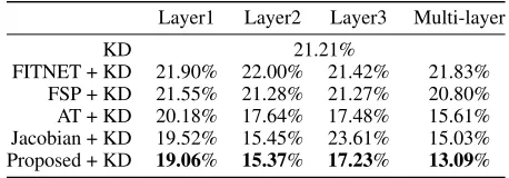
experi-Table 6: Layer-wise analysis of knowledge transfer. experi-Table shows error rate (%) of classification.

Layer1 Layer2 Layer3 Multi-layer

KD 21.21%

FITNET + KD 21.90% 22.00% 21.42% 21.83% FSP + KD 21.55% 21.28% 21.27% 20.80% AT + KD 20.18% 17.64% 17.48% 15.61% Jacobian + KD 19.52% 15.45% 23.61% 15.03% Proposed + KD 19.06% 15.37% 17.23% 13.09%

Table 7: Comparison of activation similarity withlpnorm.

Table shows percentage of same activation (%) and classifi-cation error rate (%).

l2loss l1loss l0.5loss Proposed

Layer 1 56.1% 66.9% 68.8% 96.3% Layer 2 67.3% 72.5% 73.0% 96.4% Layer 3 56.0% 56.1% 56.4% 92.8%

Error rate 10.1% 9.8% 9.6% 5.1%

ments using WRN on the CIFAR-10 dataset. In WRN, resid-ual layers are gathered to form one layer group, and three layer groups are gathered to form a network. We name the last layer of each group as layer 1, layer 2, and layer 3. The spatial sizes of these layers are 32×32, 16×16, and 8×8, respectively. Here, we regard these three layers as repsentatives for low-level, mid-level, and high-level layers, re-spectively. We analyzed the characteristics of each layer in knowledge transfer through three analytical experiments.

The first experiment is about the effect of layer-wise trans-fer. Knowledge transfer methods usually transfer multiple layer responses, but in this experiment, they are also per-formed for only a single layer to show performance differ-ences according to hidden layer location. Training was con-ducted for 120 epochs with 10% of the training data. The ex-perimental results are reported in Table 6. Most algorithms show the best performance when multiple layers are trans-ferred, but oddly, FITNET shows the best performance when only layer 3 is transferred. On the other hand, “Jacobian” has excellent performance for the mid-level layer but is not very good for the high-level layer. Conversely, AT is good for the high-level layer, but is weak for the mid-level and low-level layers. These results imply that a particular transfer method may not be good for all levels of layers. Surprisingly, how-ever, the proposed method shows the best performance in all configurations. This indicates that the proposed method is indeed suitable for transferring general neuron responses, and explains the reason for the superb performance in the previous experiments.

The second experiment is about whether the alternative loss proposed in this paper makes the neuron activations similar. For comparison, we also evaluated thel1 andl0.5 loss functions, in addition to the l2 loss. The experiment used all training data in CIFAR-10, and WRN16-4 was used for both the teacher and student networks. Here, we used the same network for both the teacher and student to

elim-Table 8: Ablation study for margin value (µ).

Margin (µ) 0.75 1 1.5 2 4

Error rate 13.9% 13.1% 12.1% 12.1% 11.7%

inate any interference caused by architectural differences. The connector functions were not used for the same reason. The experimental results are shown in Table 7. The percent-ages of neurons with the same activations in the teacher and student are presented here, and the classification errors are shown at the bottom. Since a neuron’s activation has two states, ideally, the similarity of those for a randomly initial-ized network should be 50%. Therefore, in this perspective, the l2 loss is unsuccessful in transferring the activation of neurons. Other lp losses make the activation more similar

than thel2 loss and also has better performance. However, the proposed method has much higher similarity and much better performance. This result implies that the proposed method is indeed a reasonable approximation of the ideal activation transfer loss.

The last is an ablation study on the margin valueµ, a pa-rameter of the proposed method. Although the margin value is arbitrarily set to one in other experiments, dependency of the proposed method on the margin value is an important is-sue. Experiments were performed on CIFAR-10 with 10% training data. The experimental results are shown in Table 8. Here, we can see that when the margin is larger enough, there is not much a difference in performance. The overall performance differences are not big, which means that the proposed method is not sensitive to the parameter.

Implementation Details

for the remaining epochs. In transfer learning, training was conducted for 100 epochs. For the methods requiring ini-tialization, 60 epochs were used for initialization and 40 epochs were used for classification training. AT and “Jaco-bian” were implemented to use the transfer loss, DTL loss, and cross-entropy loss simultaneously for 100 epochs. The learning rate scheme for CIFAR-10 started at learning rate 0.1 and divided the learning rate by 5 at 30%, 60%, and 80% of the total training epochs. In transfer learning, the learning rate started at 0.01 and divided by 10 when the training was over half the total epochs. In all cases, Nesterov momentum of 0.9 and a weight decay of5×10−4_{was used.}

Conclusion

Activation boundaries play an important role in neural net-works. We have investigated the role of activation bound-aries in knowledge transfer and concluded that transfer of activation boundaries can greatly enhance performance of knowledge transfer. For this purpose, we have pro-posed a knowledge transfer method by transferring activa-tion boundaries of hidden neurons. Experiments have shown that the proposed method accurately transfers the activation boundaries. At the same time, the proposed method shows much higher performance than the current state-of-the-art. In particular, in many cases of transfer learning, the pro-posed method shows better performance than ImageNet pre-training, which is a great achievement in knowledge trans-fer. In future, various tasks that originally relied on pre-training can be modified to accommodate knowledge trans-fer for better performance and learning speed. The excel-lent performance of the proposed method implies that activa-tion boundaries are indeed powerful for knowledge transfer, which can potentially change some of the essential practices of neural networks.

Acknowledgement

This work was supported by Next-Generation ICD Program through NRF funded by Ministry of S&ICT [2017M3C4A7077582] and ICT R&D program of MSIP/IITP [No.B0101-15-0552, Predictive Visual In-telligence Technology].

References

Cortes, C., and Vapnik, V. 1995. Support-vector networks. Machine Learning20(3):273–297.

Gatys, L. A.; Ecker, A. S.; and Bethge, M. 2016. Im-age style transfer using convolutional neural networks. In IEEE Conference on Computer Vision and Pattern Recogni-tion (CVPR).

He, K.; Zhang, X.; Ren, S.; and Sun, J. 2016. Deep resid-ual learning for image recognition. InIEEE Conference on Computer Vision and Pattern Recognition (CVPR).

Hinton, G.; Vinyals, O.; and Dean, J. 2015. Distilling the knowledge in a neural network. InNIPS Deep Learning and Representation Learning Workshop.

Howard, A. G.; Zhu, M.; Chen, B.; Kalenichenko, D.; Wang, W.; Weyand, T.; Andreetto, M.; and Adam, H. 2017.

Mo-bilenets: Efficient convolutional neural networks for mobile vision applications. CoRRabs/1704.04861.

Krizhevsky, A.; Sutskever, I.; and Hinton, G. E. 2012. Imagenet classification with deep convolutional neural net-works. InAdvances in Neural Information Processing Sys-tems (NIPS).

Krizhevsky, A. 2009. Learning multiple layers of features from tiny images. Technical report.

Lecun, Y.; Bottou, L.; Bengio, Y.; and Haffner, P. 1998. Gradient-based learning applied to document recognition. Proceedings of the IEEE.

Long, J.; Shelhamer, E.; and Darrell, T. 2015. Fully convolu-tional networks for semantic segmentation. InIEEE Confer-ence on Computer Vision and Pattern Recognition (CVPR). Montufar, G. F.; Pascanu, R.; Cho, K.; and Bengio, Y. 2014. On the number of linear regions of deep neural networks. In Advances in Neural Information Processing Systems (NIPS). Nair, V., and Hinton, G. E. 2010. Rectified linear units im-prove restricted boltzmann machines. InInternational Con-ference on Machine Learning (ICML).

Pan, X., and Srikumar, V. 2016. Expressiveness of rectifier networks. InInternational Conference on Machine Learning (ICML).

Pascanu, R.; Mont´ufar, G.; and Bengio, Y. 2014. On the number of inference regions of deep feed forward networks with piece-wise linear activations. InInternational Confer-ence on Learning Representations (ICLR).

Quattoni, A., and Torralba, A. 2009. Recognizing indoor scenes. InIEEE Conference on Computer Vision and Pattern Recognition (CVPR).

Romero, A.; Ballas, N.; Kahou, S. E.; Chassang, A.; Gatta, C.; and Bengio, Y. 2015. Fitnets: Hints for thin deep nets. In International Conference on Learning Representations (ICLR).

Rosasco, L.; De Vito, E.; Caponnetto, A.; Piana, M.; and Verri, A. 2004. Are loss functions all the same? Neural Computing.

Russakovsky, O.; Deng, J.; Su, H.; Krause, J.; Satheesh, S.; Ma, S.; Huang, Z.; Karpathy, A.; Khosla, A.; Bernstein, M.; Berg, A. C.; and Fei-Fei, L. 2015. ImageNet Large Scale Vi-sual Recognition Challenge. International Journal of Com-puter Vision (IJCV).

Srinivas, S., and Fleuret, F. 2018. Knowledge transfer with jacobian matching. InInternational Conference on Machine Learning (ICML).

Szegedy, C.; Liu, W.; Jia, Y.; Sermanet, P.; Reed, S.; Anguelov, D.; Erhan, D.; Vanhoucke, V.; and Rabinovich, A. 2015. Going deeper with convolutions. InIEEE Confer-ence on Computer Vision and Pattern Recognition (CVPR). Wah, C.; Branson, S.; Welinder, P.; Perona, P.; and Belongie, S. 2011. The Caltech-UCSD Birds-200-2011 Dataset. Tech-nical report.

mini-mization and transfer learning. InIEEE Conference on Com-puter Vision and Pattern Recognition (CVPR).