Ecological Modelling 146 (2001) 17 – 32
Non-spatial calibrations of a general unit model for
ecosystem simulations
Roelof M. Boumans *, F. Villa, R. Costanza, A. Voinov, H. Voinov,
T. Maxwell
Institute for Ecological Economics,P.O.Box38,Solomons,MD20657,USA
Abstract
General Unit Models simulate system interactions aggregated within one spatial unit of resolution. For unit models to be applicable to spatial computer simulations, they must be formulated generally enough to simulate all habitat elements within the landscape. We present the development and testing of a unit model for the Patuxent River landscape in the state of Maryland, USA. The Patuxent Landscape Model (PLM) is designed to simulate the interactions among physical and biological dynamics in the context of regional socioeconomic behavior. The PLM is a tool for evaluating landscape change within the Patuxent watershed through simulation of ecological systems. A companion economic model estimates land development patterns and effects on human decisions from site characteristics, ecosystem properties, and regulatory paradigms. Landscape elements that are linked within the PLM are forest, agriculture and open water systems, and three levels of urban development. Urban developments are low and medium density residential areas (14.07% of the total watershed), and commercial, industrial and institutional area (5.7%). Forests are mixed populations of deciduous and evergreen species (45.11%). Agricultural areas (28.02%) are simulated through rotating crops of corn, winter wheat and soybeans within a cycle of two years. Open water (6.84%) represents the ecosystems within the rivers and streams where phytoplankton are the primary producers. In this paper we illustrate, how we gathered and formalized working models used within the Patuxent watershed for forests, agriculture urban settings and wetlands. Further, we show how we tested and merged the variety of models employed by scientific disciplines and created a general unit model to be used in the Patuxent Landscape Model (Pat –GEM). The Patuxent Landscape Model is built under the Spatial Modeling Environment. © 2001 Elsevier Science B.V. All rights reserved.
Keywords:Ecosystem; Simulation; Complex; Calibration
www.elsevier.com/locate/ecolmodel
1. Introduction
Watersheds are composites of landscape ele-ments, which traditionally are not studied and managed in an integrated way. Foresters study forest, agriculture is the domain of farmers and
* Corresponding author. Tel.: +1-410-3267281; fax: + 1-410-3267354.
E-mail address:[email protected](R.M. Boumans).
agricultural scientists, and planners manage ur-ban areas. At a landscape scale all these man-agement objectives and scenarios for the individual landscape elements are linked.
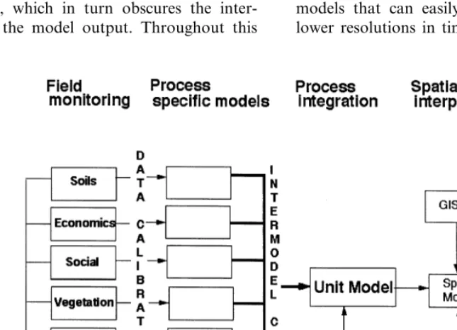
Studying the workings of systems through sci-entific observation requires recognition and for-mulation of models for hypothesis testing. The underlying objective for landscape modeling is to create tools that allow a more integrated man-agement of landscapes through simulation of in-teractions between landscape elements. To go from specialized management to a more inte-grated approach, the gap between the working models of observers specialized in single land-scape elements and the entire landland-scape needs to be bridged (Fig. 1).
Computer landscape simulation is a logical method for the integrated approach between dis-ciplines due to its ability to handle large amounts of data and information and to provide output aggregated for easy interpretation. The complexity introduced with large amounts of data and information very likely creates non-lin-ear behavior, which in turn obscures the inter-pretation of the model output. Throughout this
paper we present how confidence can be gained for simulation results from complex unit models.
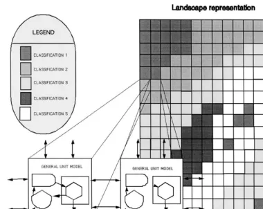
1.1. General unit models
Landscape simulations require the formulation of general unit models for simulation of tempo-ral processes (Fig. 2; Fitz et al., 1995). Dynam-ics for general models are by definition not habitat specific. Discrimination between habitats is accomplished by applying habitat specific ini-tializations of stocks and parameters. General models in contrast to unique habitat specific models, ease the computational challenges in representing landscape dynamics at the higher resolutions (Fitz et al., 1995; Running and Coughlan, 1988; Running and Gower, 1991; Parton et al., 1994). Landscape models that do not make use of general models often are spe-cialized for one habitat (e.g. forest models; Run-ning and Gower, 1991; Band et al., 1991) or assume large aggregations of the landscape (Baker, 1989). The challenge is to create unit models that can easily be scaled to higher and lower resolutions in time and space.
R.M.Boumans et al./Ecological Modelling146 (2001) 17 – 32 19
Fig. 2. Schematic of a landscape model.
1.2. Model description
Pat –GEM was developed to be the ecological model and non-spatial building unit for the spa-tial Patuxent Landscape Model (PLM). PLM cov-ers ecological-economic dynamics of the 2500 km2
Patuxent river watershed in Maryland and inte-grates data and knowledge over several spatial, temporal and complexity scales in order to aid regional management. The PLM effort is an out-growth of a model first developed for Louisiana wetlands and later expanded and applied to the Florida Everglades (Costanza et al., 1990; Fitz and Sklar, 1999). PLM is the first implementation of the full ecological model in an upland setting and includes hydrology, nutrients, plants, animal populations, and human economic systems. The landscape is depicted as a grid of cells with a minimum cell size of 200×200 m2 to allow
ade-quate depiction of the pattern of ecosystem pro-cesses and human settlement on the landscape.
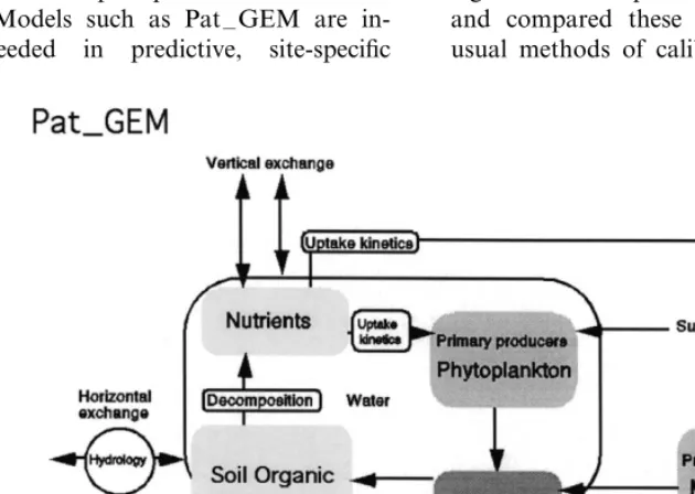
Pat –GEM includes modules for hydrology, nu-trient movement and cycling, terrestrial and estu-arine primary productivity, and general consumer dynamics (Fig. 3). The hydrology module of the unit model is a fundamental component for other modeled processes, simulating water flow verti-cally within the cell (e.g. infiltration, evapotran-spiration). Phosphorus and nitrogen are cycled through plant uptake and organic matter decom-position, with the latter simulated in a sediment/
plant and phytoplankton growth in response to available sunlight, temperature, nutrients, and water;
animal (consumers) growth in response to food sources;
dynamics in detrital matter; dynamics in soil organic matter;
flow of water plus dissolved nutrients in three dimensions.
Feedbacks among the biological, chemical and physical model components are important struc-tural attributes to the model. While the unit model simulates ecological processes within a unit cell, horizontal fluxes link the cells together across the landscape to form the full landscape model. These spatial fluxes are driven by cell-to-cell head differences of surface and ground water in satu-rated storage. Water fluxes between cells carrying dissolved and suspended materials for simulating water quality in the landscape.
1.3. Calibration/6erification of unit models
Pat –GEM is a complex process-based simula-tion model. Models such as Pat –GEM are in-creasingly needed in predictive, site-specific
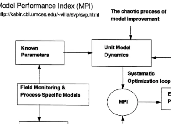
environmental research (Band et al., 1993; Costanza et al., 1993; Wigmosta et al., 1994; Baron et al., 1998; Creed and Band, 1998). In-creasing complexity causes the number of solu-tions within the parameter space to grow exponentially with the number of unknown parameters, and finding a unique solution through calibration at the complexity of Pat –GEM, with 21 state variables and 37 unknown parameters, is virtually impossible (Beven and Binley, 1992; Beven, 1993). Instead of narrowing down to one unique solution within the parameter space, we applied whole system tests for conservation of mass and robust behavior, and applied a newly developed Model Performance Index (MPI) (Fig. 4). We also utilized a set of exploratory tech-niques (Villa et al., 2001) to isolate multiple areas within the parameter-space that produce agree-ments between model simulation output and available systems information.
Theoretical problems with calibrating complex models is highlighted by Villa et al. (1998) who developed and applied a computer aided search algorithm for exploring model parameter spaces, and compared these explorations against more usual methods of calibration such as eyeballing,
R.M.Boumans et al./Ecological Modelling146 (2001) 17 – 32 21
Fig. 4. Calibration process using MPI and systematic optimizations of unknown parameters to improve confidence in unit model performance.
hill climbing and Monte Carlo experiments. Villa et al. (1998) found that as the number of un-known parameters increases, the number of areas that can be discriminated within the parameter space to fit the same observed data is also increas-ing. When less is known of a modeled system, systematic calibration of complex models will re-veal more potential solutions. Consequently, non-systematic calibrations, such as ‘eye balling’, have been inconclusive as methods for exploring the total potential parameter space.
2. Methods
2.1. Model applied
Pat –GEM was developed from the GEM model presented by Fitz et al. (1995). Develop-ment of the GEM was mostly for simulating wetland dynamics, emphasizing and elaborating on water column dynamics in mostly estuarine environments. With Pat –GEM we shifted focus to the dynamics of more terrestrial and human dominated habitats such as forests, agricultural lands and urban areas. This shift in focus not only required changes to settings of the parameter
values, but also brought about more general ap-proaches regarding how these parameters influ-enced the ecosystem properties. Applying the GEM model to additional alternative settings will continue this generalization process of modeling ecosystem processes.
The important objective after constructing Pat – GEM was to gain confidence in simulation out-puts for mimicking the ecological, physical and biological processes that are of importance to the dynamics within the Patuxent watershed. Apply-ing innovative strategies for unit model calibra-tion, we learned about the limits of applicability and the range of behaviors exhibited by Pat – GEM, and we narrowed down the areas in the parameter space that are most likely to represent Patuxent watershed habitats. We discovered tem-poral scalability variations among variables and tested for conservation of materials.
2.2. Robustness
model was calibrated, were regressed against the one-day time step output (Table 1).
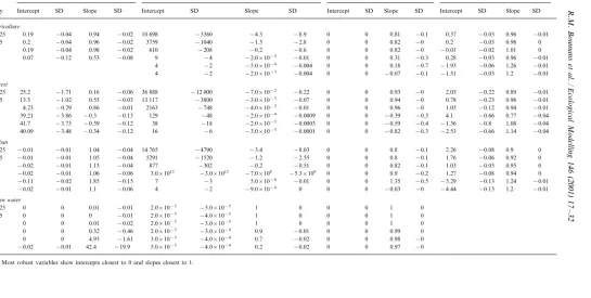
Poorly robust behavior in some of the state variables such as nitrogen did not cause similar poor behavior in state variables that track long term changes within a system such as soil organic matter in terrestrial ecosystems. Overall, state variables with low frequency dynamics were most predictable. Table 1 shows the results of the ro-bustness tests for a selection of Pat –GEM state variables. Robust behavior varied between state variables and within state variables among lan-duses. For example, biomass in agricultural land uses could be reproduced at the higher resolution time steps (intercept 0, slope 1), but missed the day on which farmers planted crops at lower resolutions. The deciduous nature of the forest proved forest biomass to be time step sensitive due to the fast processes during the short periods of the year of greening up and litterfall. In com-parison, urban lawns were more robust. The least robust was the biomass stock in open water habi-tat that is mainly modeled as phytoplankton, a biomass stock very sensitive to erratic behavior in surface water nutrient concentrations.
Interesting differences in robust behavior are illustrated by the two nutrients, nitrogen and phosphorous. While phosphorous behaves fairly robustly, nitrogen performed poorly. Pat –GEM recognizes the immobile stage of inorganic phos-phorous in the soil, but not of nitrogen. Conse-quently, nitrogen concentrations are more sensitive to hydrologic events which are fast paced, in comparison to the buffered phospho-rous concentrations.
2.3. Conser6ation of materials
Pat –GEM was tested for conservation of mate-rials. Pat –GEM lumps organic carbon, nitrogen and phosphorous within the state variable ‘biomass’, while accounting separately for inor-ganic nitrogen and phosphorous. Conversions be-tween organic and inorganic states are derived through assigning parameters for carbon to nitro-gen to phosphorous ratios. Unless materials are represented by state variables through all configu-rations (e.g. inorganic and organic states),
calibra-tion of C:N:P ratios are required to balance material influxes, outfluxes and stocks to comply with the law of conservation of mass. In Pat – GEM, no state variables are assigned to variation in inorganic carbon, nor are the dynamics of oxygen and trace minerals included.
Calibrations carried out for forest simulations showed that nutrient ratio parameters could be found to ensure conservation of mass within an acceptable margin of error. After calibration, losses or gains never exceeded 0.0012% for phos-phorous or 0.0002% for nitrogen at any time during a two-year simulation. Regrettably, these calibrated results were very sensitive to new set-tings in other areas of the parameter space so that re-calibration of the nutrient ratios is required for each new implementation of the model.
Although material ratios in phytoplankton are considered very stable (e.g. Redfield ratios) other systems have worked out mechanisms to concen-trate nutrients in the living part of the organic matter while depleting the non-living part. For example, nutrients in trees are concentrated under the bark and in the leaves. When this tissue dies and becomes wood, nutrients are recovered for use by non-woody parts. A similar recapturing of nutrients takes place during coloring and shed-ding of leaves in the fall. From this example, we learn that when forests grow in age (more stand-ing wood) nutrient to carbon ratios decline (Par-ton et al., 1988; Vitousek et al., 1988). Increase in nutrient ratios occur within the transformation from detritus to soil organic matter. Given the right temperature and moisture conditions the microbial organisms that carry out the decompo-sition will sequester the nutrients while respiring the carbon causing a change in nutrient ratios.
2.4. Exploration of the parameter space
R
.
M
.
Boumans
et
al
.
/
Ecological
Modelling
146
(2001)
17
–
32
23
Table 1
Model output from simulations diverting from the one-day time step for which Pat–GEM was calibrated, were regressed against the one-day time step outputa
Biomass
DT Inorganic nitrogen Inorganic phosphor Soil organic matter
Intercept SD Slope SD Intercept SD Slope SD Intercept
Day SD Slope SD Intercept SD Slope SD
Agriculture
0.19 −0.04 0.94
0.125 −0.02 10 698 −3360 −4.3 −8.9 0 0 0.81 −0.1 0.37 −0.03 0.96 −0.01
0.2 −0.04 0.96 −0.02 3759 −1040 −1.5 −2.8
0.25 0 0 0.82 −0 0.2 −0.03 0.98 0
0.5 0.19 −0.04 0.98 −0.02 610 −208 −0.2 −0.6 0 0 0.82 −0 −0.01 −0.02 1.01 0 0.07 −0.12 0.53 −0.08 9 −4 −2.0×10⁻³ −0.01 0 0 0.31 −0.3 0.28 −0.03
2 0.96 −0.01
4 −2 −5.0×10⁻⁴ −0.004
4 0 0 0.18 −0.7 −1.93 −0.06 1.26 −0.01
8 4 −2 −2.0×10⁻³ −0.004 0 0 −0.07 −0.1 −1.51 −0.05 1.2 −0.01
Forest
25.2 −1.71 0.16 −0.06 36 888 −12 000 −7.0×10⁻² −0.22 0 0 0.93 −0 2.03 −0.22 0.89
0.125 −0.01
13.5 −1.02 0.55 −0.03 13 117 −3800 −3.0×10⁻² −0.07
0.25 0 0 0.94 −0 0.78 −0.23 0.96 −0.01
4.23 −0.29 0.86 −0.01 2163 −748 −4.0×10⁻³ −0.01
0.5 0 0 0.96 −0 1.05 −0.12 0.94 −0.01
39.21 −3.86 −0.3 −0.13 129 −48 −2.0×10⁻⁴ −0.0009
2 0 0 −0.39 −0.3 4.1 −0.66 0.77 −0.04
41.7 −3.75 −0.39 −0.12 38 −18 −2.0×10⁻⁵ −0.0003 0 0 −0.59 −0.4 −1.36 −0.8 1.08
4 −0.04
40.09 −3.48 −0.34 −0.12 16 −6 −3.0×10⁻⁵ −0.0001
8 0 0 −0.82 −0.3 −2.53 −0.66 1.14 −0.04
Urban
−0.01 −0.01 1.04 −0.04 14 765 −4790 −3.4 −8.03
0.125 0 0 0.8 −0.1 2.26 −0.08 0.9 0
−0.01 −0.01 1.05 −0.04 5291 −1520 −1.2 −2.55 0 0 0.8 −0.1 1.76 −0.06 0.92
0.25 0
−0.02 −0.01 1.13 −0.04 877 −302 −0.2 −0.51
0.5 0 0 0.82 −0.1 1.03 −0.03 0.95 0
−0.02 −0.01 1.06 −0.06 3.0×10¹² −3.0×10¹² −7.0×10⁸ −5.3×10⁹
2 0 0 0.9 −0.2 1.27 −0.08 0.94 0
−0.11 −0.02 1.85 −0.15 7 −3 5.0×10⁻⁴ −0.01
4 0 0 1.35 −0.5 −5.29 −0.13 1.24 −0.01
−0.02 −0.01 1.1 −0.06 4 −2 −9.0×10⁻⁴ 0 0
8 0 −0.03 −0 −4.44 −0.13 1.2 −0.01
Open water
0 0 0.01 −0.01 2.0×10⁻⁵ −5.0×10⁻⁵
0.125 1 0 0 0 1 0
0 0 0 −0.01 2.0×10⁻⁵ −4.0×10⁻⁵
0.25 1 0 0 0 1 0
0 0 0.01 −0.02 2.0×10⁻⁵ −3.0×10⁻⁵ 1 0
0.5 0 0 1 0
2 0 0 0.32 −0.46 2.0×10⁻³ −3.0×10⁻⁴ 0.9 −0.01 0 0 0.99 0
0 0 4.93 −1.61 3.0×10⁻³ −4.0×10⁻⁴ 0.7 −0.02
4 0 0 0.98 −0
8 −0.02 −0.01 42.4 −19.9 5.0×10⁻³ −4.0×10⁻⁴ 0.2 −0.02 0 0 0.97 −0
parameters, to obtain maximal calibration effi-ciency and highlight feasible areas on which to concentrate investigation.
To carry on this investigation, we exploited the Model Performance Index framework described in Villa et al. (1998). This framework allows the definition of a model’s parameters function (from now on called the objective function) expressing the agreement of quantitative data and semi-quantitative hypotheses about the model’s ex-pected behavior with the model’s output. MPI-based objective functions are used to explore the parameter space under different viewpoints, from simple feasibility of the output to exact matching of particular data sets. A number of search techniques were used, from Monte Carlo exploration to global optimizations using genetic algorithms.
The sensitivity of the MPI scores for state variables to particular individual parameters is very dependant upon a total configuration of the objective function, and no general conclusion can be drawn about the effect of parameter changes without considering this overall objective function context. But simply knowing the proportion of cases that particular parameters were influential for changes to state variables for many configura-tions of the objective function is obviously impor-tant to the investigator. The influence plot in Fig. 5 shows this proportion for single parameter ef-fects and two-way interaction efef-fects. The effect of each parameter is detailed for each single vari-able. As the plot shows, most effects are signifi-cant only in a minority of cases, which further demonstrates the complex nature of the model’s response. However, some parameters seem to infl-uence the variables’ MPIs in most cases. With the help of the influence plot, the experimenter can check at a glance whether a change in a parameter is likely to improve the MPI score for a variable, which other variables are likely to be involved, and which other parameters are likely to be in-volved in the effect. This proves to be essential in forming the next step in the calibration process. Parameters which do not seem to have an effect can be excluded from the next search to save on computational time, using their maximum likeli-hood estimates. Parameters and their interactions
which appear to have an effect in the majority of cases can be further investigated until a better calibration point is found. This can be used as the initial guess for a new automated search cycle, maybe with redefined parameter boundaries and sensitivities to narrow the search space.
2.5. Calibration experiments
During the analysis of many search cycles, Ex-ploratory Data Analysis (EDA) techniques and careful use of data reduction are useful to over-come the complexity due to the multivariate na-ture of the response surface. To help this process, we have designed a suite of tools, which quickly allow us to interactively generate specific plots according to specific needs. After determining that the combined effect of two parameters is worth exploring by looking at the influence plot, more quantitative knowledge about these particular ef-fects can be sought by plotting the MPI values as a function of parameter value.
We explored the potential for subdivision of the parameter space to carry out multiple calibrations at reduced complexities. Subsets in the parameter space were identified, and parameters clustered around their most likely to be influenced vari-ables. In addition, we separated those parameters that introduced the highest levels of complexity and gave them fixed values to simplify analysis of the remaining parameter space.
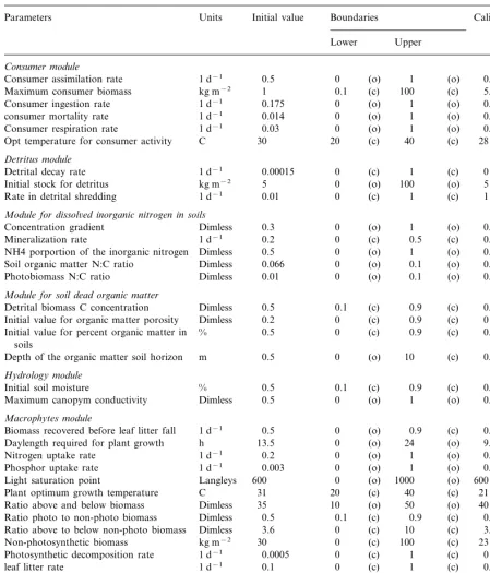
Initially, a large sample of 71 from the 128-di-mensional PLM parameter space was selected for exploration. Parameter space dimensions that in-volved processes between cells (spatial parameters exclusively linked to hydrology), parameters de-signed for specific scenarios, and parameters in-volved in processes that are not likely to be within a forested habitat at the 200 m resolution were not explored. The 71 parameters were assigned maximum and minimum boundaries and sub-jected to an initial exploration for sensitivity using genetic algorithms (Wang, 1997). An additional 43 parameters were excluded when they proved to be insensitive on the overall modeling results.
al-R.M.Boumans et al./Ecological Modelling146 (2001) 17 – 32 25
gorithms to fit the GEM models against measured data. As we explored a remaining 37-dimensional parameter space (Fig. 5; Table 2), we found macrophyte variables for Net Primary Productiv-ity and Leaf Area Index (Fig. 6) most sensitive to parameter changes. Variables and test criteria se-lected are presented in Table 3. Least sensitive were material fluxes associated with mortality of
photosynthetic and non-photosynthetic macro-phyte biomass, the translocation of photosyn-thetic materials from the leaves to the roots, and the stock in non-photosynthetic carbon. Some sensitivity was observed for consumption of non-photosynthetic tissues.
We found that the Leaf Area Index in the PLM is most efficiently calibrated using single
Table 2
Pat –GEM parameter valuesa
Initial value Boundaries
Parameters Units Calibrated value
Lower Upper
Consumer module
Consumer assimilation rate 1 d−1 0.5 0 (o) 1 (o) 0.15
1 0.1
Maximum consumer biomass kg m−2 (c) 100 (c) 5.9895
0.175 0 (o) 1
1 d−1 (o)
Consumer ingestion rate 0.175
1 d−1
consumer mortality rate 0.014 0 (o) 1 (o) 0.003
Consumer respiration rate 1 d−1 0.03 0 (o) 1 (o) 0.03
30 20 (c) 40 (c)
C 28
Opt temperature for consumer activity
Detritus module
0.00015 0 (c) 1 (c) 0
Detrital decay rate 1 d−1
5 0 (o) 100
kg m−2 (o)
Initial stock for detritus 5
Rate in detrital shredding 1 d−1 0.01 0 (c) 1 (c) 1
Module for dissol6ed inorganic nitrogen in soils
0.3 0
Concentration gradient Dimless (o) 1 (o) 0.8
0.2 0 (c) 0.5
1 d−1 (c)
Mineralization rate 0.5
Dimless
NH4 porportion of the inorganic nitrogen 0.5 0 (o) 1 (o) 0.5 Dimless
Soil organic matter N:C ratio 0.066 0 (o) 0.1 (o) 0.067
0.01 0 (o) 0.1
Dimless (o)
Photobiomass N:C ratio 0.001
Module for soil dead organic matter
0.5 0.1 (c) 0.9
Dimless (c)
Detrital biomass C concentration 0.42
Initial value for organic matter porosity Dimless 0.2 0 (c) 0.9 (c) 0
% 0.5 0 (c) 0.9
Initial value for percent organic matter in (c) 0.05
soils
m
Depth of the organic matter soil horizon 0.5 0 (o) 10 (c) 0.5
Hydrology module
0.5 0.1
Initial soil moisture % (c) 0.9 (c) 0.3008
Maximum canopym conductivity Dimless 0.5 0 (o) 1 (o) 0.5
Macrophytes module
0.5 0 (o) 0.9
1 d−1 (c)
Biomass recovered before leaf litter fall 0.5
h
Daylength required for plant growth 13.5 0 (o) 24 (o) 9.42 0.2
Nitrogen uptake rate 1 d−1 0 (o) 1 (o) 0.15
0.003 0 (o) 1
1 d−1 (o)
Phosphor uptake rate 0.003
Langleys
Light saturation point 600 0 (o) 1000 (o) 600
C
Plant optimum growth temperature 31 20 (c) 40 (c) 21
35 10 (o) 50
Dimless (o)
Ratio above and below biomass 40
0.5 0.1 (c) 0.9 (c) 0.5
Ratio photo to non-photo biomass Dimless
3.6 0 (c) 10
Dimless (c)
Ratio above to below non-photo biomass 3.6
kg m−2
Non-photosynthetic biomass 30 0 (c) 100 (c) 23
Photosynthetic decomposition rate 1 d−1 0.0005 0 (c) 1 (c) 0
0.1 0 (c) 1 (c)
1 d−1 0.99
leaf litter rate
Module for soil phosphor
0.0108 0.01 (c) 0.09 (c) 0.01 Photobiomass P:C ratio Dimless
0.3 0 (c) 0.9
Dimless (c)
Concentration gradient 0.3
kg m−3
Equilibrium conc. for mobile phosphor 0.03 0 (o) 0.1 (c) 0.03
0.003 0 (c)
Initial concentration kg m2−2 1 (c) 0
0.2 0 (o) 1
1 d−1 (c)
Absorption rate for mobile phosphor 0.2
R.M.Boumans et al./Ecological Modelling146 (2001) 17 – 32 27
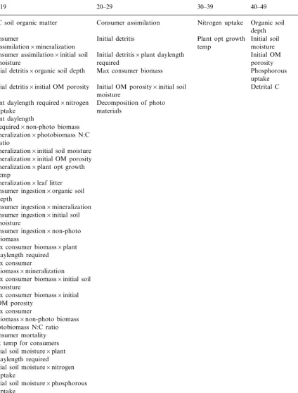
ters within the macrophyte module. We also found important parameter interactions between the con-sumer and macrophyte modules, soil organic mat-ter and macrophyte modules, and among macrophyte parameters. Table 4 shows the fre-quency distribution of single parameters and
parameter combinations.
Net Primary Productivity is sensitive to single parameters within the macrophyte, soil organic matter, consumer and nitrogen modules. Important parameter interactions occur between the macrophyte and consumer modules, soil organic
Fig. 6. Panel A shows the most successful parameter update sequence during the execution of the MPI search algorithm for Pat –GEM forest applications. Individual variable agreements with assigned test requirements (partial MPI) are evaluated against collective variable test agreement (global MPI). Panel B shows model agreement between NDVI values and Net Primary Productivity after eyeballing (the initial guess), after the most successful update sequence (MPI=0.29), and after a less successful update sequence (MPI=0.13).
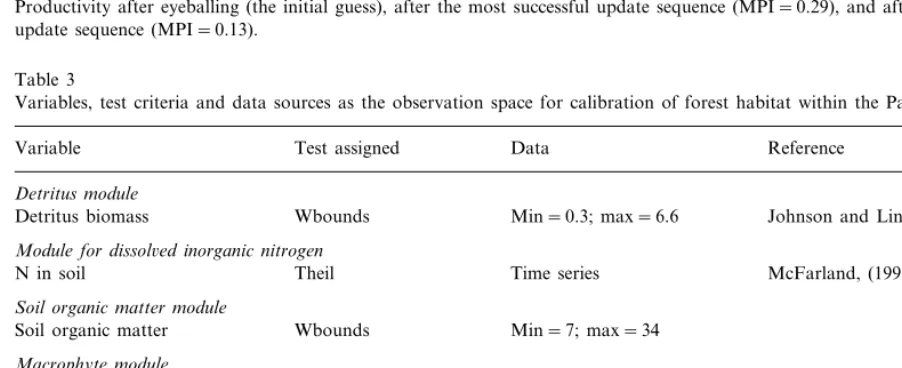
Table 3
Variables, test criteria and data sources as the observation space for calibration of forest habitat within the Pat –GEM
Reference Test assigned
Variable Data
Detritus module
Wbounds Min=0.3; max=6.6
Detritus biomass Johnson and Lindberg, (1992)
Module for dissol6ed inorganic nitrogen
N in soil Theil Time series McFarland, (1995)
Soil organic matter module
Soil organic matter Wbounds Min=7; max=34
Macrophyte module
Wbounds Min=0; max=9 Johnson and Lindberg, (1992) Leaf area index
Wbounds
Non-photo biomass Min=2.5; max=42 FIA database
Wbounds
Photo biomass Min=0.1; max=3.5 FIA database
NDVI Time series
Net primar prod. Freq
Phosphor module
Table 4
Frequency distributions of single parameters and parameter combinations
10–19 20–29 30–39 40–49 50–60
Nitrogen uptake
N:C soil organic matter Consumer assimilation Organic soil Plant daylength required depth
Initial detritis Plant opt growth Initial soil Mineralization Consumer
temp
assimilation×mineralization moisture
Initial detritis×plant daylength Initial OM Non-photo Consumer assimilation×initial soil
moisture required porosity biomass
Initial detritis×organic soil depth Max consumer biomass Phosphorous Leaf litter uptake
Initial OM porosity×initial soil Detrital C Initial detritis×initial OM porosity
moisture
Plant daylength required×nitrogen Decomposition of photo
uptake materials
Plant daylength
required×non-photo biomass Mineralization×photobiomass N:C
ratio
Mineralization×initial soil moisture Mineralization×initial OM porosity Mineralization×plant opt growth
temp
Mineralization×leaf litter Consumer ingestion×organic soil
depth
Consumer ingestion×mineralization Consumer ingestion×initial soil
moisture
Consumer ingestion×non-photo biomass
Max consumer biomass×plant daylength required
Max consumer
biomass×mineralization Max consumer biomass×initial soil
moisture
Max consumer biomass×initial OM porosity
Max consumer
biomass×non-photo biomass Photobiomass N:C ratio Consumer mortality Opt temp for consumers Initial soil moisture×plant
daylength required Initial soil moisture×nitrogen
uptake
Initial soil moisture×phosphorous uptake
Max canopy conductivity Initial OM porosity×plant
daylength required
Initial OM porosity×plant opt. growth temp
Initial OM porosity×non-photo biomass
R.M.Boumans et al./Ecological Modelling146 (2001) 17 – 32 29
matter and nitrogen modules, detritus and hydrology modules, and among macrophyte module parameters.
2.6.Pat–GEM calibrations for four habitats within
the Patuxent watershed
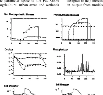
PLM land uses are aggregated into six separate categories of which three are within different urban settings. Unit model calibrations explored the parameter space to represent characteristics found in forest, agriculture, open water and urban set-tings. The paper presents only examples carried out for forests. Data sources upon which we have based our assumptions for correct model behavior are presented in Table 2. Explorations on relevant areas in the parameter space of the Pat –GEM model for agricultural urban areas and wetlands
are within various stages of completion (Fig. 7). Development and calibration of General Ecosys-tem Models runs parallel to the advancements that take place within the various fields of science dedicated to individual habitat types. Changes in paradigms will lead to the adjustment of General Ecosystem Model dynamics, while new observa-tional information on parameters will further nar-row our unknown parameter space. New observations in time and space will expand the test criteria that are available for calibration.
3. Discussion
We presented methods and results that were designed to help increase and report the confidence in output from models that are too complex for
applying conventional means of calibration and verification. Our model, derived from less complex models based upon careful observation of time and space specific phenomena, is intended for simulat-ing ecological processes in the Patuxent watershed. The attempt to cover within one model, all poten-tial habitats under all conditions not only caused expansions in the unknown area of the parameter space, but also reached levels of complexity and non-linear behavior such that conventional tech-niques for means of building confidence were inappropriate. Through our experiments, invalu-able information was gathered on how to improve complex model calibrations and report the results objectively.
Confidence levels remained low after applying the tests on conservation of mass. Pat –GEM is intended for use in spatial modeling, where each pixel in the landscape represents a unique combina-tion of parameters. Addicombina-tional calibracombina-tion to have each unique combination meet conservation of mass requirements is cumbersome. The question is raised as to whether the computational benefits expected from lumping the organic nutrient frac-tions in the biomass weights justify the calibration efforts that are needed to satisfy the law of conser-vation of mass. The error can be noted but ignored assuming the existence of a non-modeled nutrient pool that functions as capacitor. A likely candidate for the function could be the non-modeled micro-bial biomass.
Confidence gained from the parameter search routines was subject to pre-calibration conditions of the availability and quality of the information and data available for testing. Reporting this sub-jectivity provided the means upon which confidence levels between complex models can be compared. Before testing a complex model such as Pat –GEM, an observational space will need to be defined. Testing output against observations is the most powerful means to gain confidence in model predic-tions. The Pat –GEM model potentially can be tested against 76 different categories of observa-tions (total sum of stocks and fluxes) and most confidence would be gained when all stocks and fluxes would agree with data from observations. Unfortunately, for a large subset of the 76 stocks and flows in the Pat –GEM, there were no
observa-tions, no data from observaobserva-tions, or no compatible data from observations. Good agreement on a few categories of observational data could give a false sense on the complete goodness-of-fit when other properties of the model were not tested at all.
A calibration specific formulation of the MPI is defined within an a priori observational space, not only in quantity, e.g. how many of the stocks and flows are being tested, but also in quality. Quality statements are for the individual fluxes or stocks and are imbedded when a particular statistical test is assigned, as well as in the weighting of the test results in the ultimate index. For example, more confidence is gained when one of the model outputs is able to track a time series expressed in compatible units, measured at time intervals similar to the model time step (thiel test), than when a particular model output is not exceeding boundary conditions (boundary test). On the other hand, if the data quality of the time series is questionable while the boundary conditions are firm, more confidence should be assigned to the results of the boundary test.
3.1. The narrowing of the parameter space
Confidence can be gained for complex simulation models when the objective function can be reduced to only the most important dimensions. Villa et al. (1998) found that with increasing numbers of unknown parameters the number of potential areas in the parameter space for fitting the model output to the observational space also increased. Although this opens up an important discussion on how natural phenomena classified similarly through observation can have very different underlying dynamics and building confidence in the model output requires systematic narrowing of the parameter space before calibration. How the parameter space is narrowed is important informa-tion for judging calibrainforma-tions. As in defining the observational space, the a priori explanation of the quality and quantity of the known parameter space and how non-relevant and insensitive parameters are identified create yet another dimension to the confidence level expectancy.
R.M.Boumans et al./Ecological Modelling146 (2001) 17 – 32 31
surprises for the remaining parameters and parameter variable interactions with respect to the literature on forest dynamics (Gholtz et al., 1994; Reichle, 1981; Vitousek et al., 1988). After assign-ing values to 34 parameters to be known of no consequence to either forest or non-spatial dy-namics, we were still left with 37 unknown parameters. Because Villa et al. (1998) found in the complex model they explored, a maximum allowable number of nine unknown parameters, we searched the records on the successful hill climbing attempt for those parameters that were most influential for improving upon the overall MPI score (Fig. 5). Different definitions of the observation space undoubtedly will expose differ-ent sets on infludiffer-ential parameters. Extra confi-dence is gained when calibrations for observational spaces, defined within habitat, bring forward tendencies in parameter variable interac-tions that can be recognized by habitat experts.
4. Final conclusion
More detailed classification through hierarchi-cal schemes applied to landscape models (Mitsch, 1992; Lavorel et al., 1995; Michaelsen et al., 1994) will have to be followed up with more specific calibrations of complex unit models. Not only will we want a calibration for a generic forest; eventu-ally we will want to know about available obser-vations, objective function reductions and attainable MPI scores for deciduous and conifer-ous forests.
References
Baker, W.L., 1989. A review of models of landscape change. Landscape Ecology 2 (2), 111 – 133.
Band, L.E., Patterson, P., Nemani, R., Running, S.W., 1993. Forest ecosystem processes at the watershed scale-incorpo-rating hillslope hydrology. Agricultural and Forest Meteo-rology 63 (1 – 2), 93 – 126.
Band, L.E., Peterson, D.L., Running, S.W., Coughlan, J., Lammers, R., Dungan, J., Nemani, R., 1991. Forest ecosystem processes at the watershed scale basis for dis-tributed simulation. Ecological Modelling 56, 171 – 196. Baron, J.S., Hartman, M.D., Kittel, T.G.F., Band, L.E.,
Ojima, D.S., Lammers, R.B., 1998. Effects of land cover,
water redistribution, and temperature on ecosystem pro-cesses in the South Platte Basin. Ecological Applications 8, 1037 – 1051.
Beven, K., 1993. Prophecy, reality and uncertainty in dis-tributed hydrological modelling. Advances in Water Re-sources 16, 41 – 51.
Beven, K., Binley, A., 1992. The future of distributed models: model calibration and uncertainty prediction. Hydrological Processes 6, 279 – 298.
Costanza, R., Sklar, F.H., White, M.L., 1990. Modeling coastal landscape dynamics. BioScience 40, 91 – 107. Costanza, R., Wainger, L., Folke, C., Maler, K.-G., 1993.
Modeling complex ecological and economic systems: to-wards an evolutionary, dynamic understanding of people and nature. BioScience 43 (8), 545 – 555.
Creed, I.B., Band, L.E., 1998. Exploring functional similarity in the export of nitrate-N from forested catchments: a mechanistic modeling approach. Water Resources Re-search 34, 3079 – 3093.
Fitz, H.C., DeBellevue, E., Costanza, R., Boumans, R., Maxwell, T., Wainger, L., Sklar, F., 1995. Development of a general ecosystem model for a range of scales and ecosystems, Ecological Modelling.
Fitz, H.C., Sklar, F.H., 1999. Ecosystem analysis of phospho-rus impacts and altered hydrology in the everglades: a landscape modeling approach. In: Reddy, K.R., O’Con-nor, G.a., Schelske, C.L. (Eds.), Phosphorus Biogeochem-istry in Subtropical Ecosystems. Lewis Publishers, Boca Raton, FL, pp. 585 – 620.
Gholtz, H.L., Linder, S., McMurtrie, R.E., 1994. Environmen-tal Constraints on the Structure and Productivity of Pine Forest Ecosystems: a Comparative Analysis. Munksgaard, Copenhagen.
Johnson, D.W., Lindberg, S.E., 1992. Atmospheric Deposition and Forest Nutrient Cycling: a Synthesis of the Integrated Forest Study. Springer, New York.
Lavorel, S., Gardner, R.H., O’Neill, R.V., 1995. Dispersal of annual plants in hierarchically structured landscapes. Landscape Ecology 10 (5), 277 – 289.
McFarland, E.R., 1995. Relation of Land Use to Nitrogen Concentration in Ground Water in the Patuxent River Basin Maryland, USGS Report.
Michaelsen, J., Schimel, D.S., Friedl, M.A., Davis, F.W., Dubayah, R.C., 1994. Regression tree analysis of satellite and terrain data to guide vegetation sampling and surveys. Journal of Vegetation Science 5, 673 – 686.
Mitsch, W.J., 1992. Combining ecosystem and landscape ap-proaches to Great Lakes wetlands. Journal of Great Lakes Research 18 (4), 552 – 570.
Parton, W.J., Stewart, J.W.B., Cole, C.V., 1988. Dynamics of C, N, P, and S in grassland soils: a model. Biogeochemistry 5, 109 – 131.
Reichle, D.E., 1981. Dynamic Properties of Forest Ecosys-tems. Cambridge University Press, New York.
Running, S.W., Coughlan, J.C., 1988. A general model of forest ecosystem processes for regional applications 1. Hy-drologic balance, canopy gas exchange and primary pro-duction processes. Ecological Modelling 42, 125 – 154. Running, S.W., Gower, S.T., 1991. Forest-BGG. A general
model of forest ecosystem processes for regional applica-tions. II. Dynamic carbon allocation and nitrogen budgets. Tree Physiololgy 9, 147 – 160.
Villa, F., Boumans, R.M.J., Costanza, R., 1998. Calibration and testing of complex process-based simulation models. Proceedings of the Applied Modeling and Simulation (AMS) Conference, Honolulu, 12 – 14 August 1998.
Villa, F., Boumans, R.M.J., Costanza, R., 2001. Design and use of a model performance index (MPI) for the calibra-tion of ecological simulacalibra-tion models. Submitted for publi-cation.
Vitousek, P.M., Fahey, T., Johnson, D.W., Swift, M.J., 1988. Element interactions in forest ecosystems: succession, al-lometry, and input – output budgets. Biogeochemistry 5, 7 – 34.
Wang, Q.L., 1997. Using generic algorithms to optimise model parameters. Environmental Modeling and Software 12 (1), 27 – 34.