Web Ecology 8: 22–29.
Species distributional models based on lattice data often display spatial autocorrelation. Spatial autocorrelation means that observations from nearby locations are often more similar than would be expected on a random basis (Legendre and Legendre 1998). Spatial autocorrelation can arise in both species distributions and environmental variables. Note that statistical analyses of such data need not be seen as problematic in principle. However, a chosen method is inconsistent with its application, if and only if (1) these autocorrelated variables lead to autocorrelated er-rors and (2) independently and identically distributed (i.i.d.) errors are assumed in the used statistical model. In that case results of the method are not reliable (Kühn 2007).
There are several reasons for autocorrelated errors in linear regressions (Kissling and Carl 2008). (1) Response variables, e.g. species distributions are spatially structured due to endogenous properties such as, e.g. dispersal, speci-ation, and extinction. Because structure is only inherent in the response variable, it can not be explained by explanato-ry environmental variables. Therefore, it leaves its mark on the regression errors. (2) Response variables are spatially structured due to exogenous properties such as specific en-vironmental variables, e.g. wind or other climatic con-straints. In the model, however, the very same variables are either not included or improperly used due to neglected non-linear transformations. Here the spatial structure, in turn, affects the errors.
A wavelet-based method to remove spatial autocorrelation in the
analysis of species distributional data
Gudrun Carl, Carsten F. Dormann and Ingolf Kühn
Carl, G., Dormann, C. F. and Kühn, I. 2008. A wavelet-based method to remove spa-tial autocorrelation in the analysis of species distributional data. – Web Ecol. 8: 22–29.
Species distributional data based on lattice data often display spatial autocorrelation. In such cases, the assumption of independently and identically distributed errors can be violated in standard regression models. Based on a recently published review on meth-ods to account for spatial autocorrelation, we describe here a new statistical approach which relies on the theory of wavelets. It provides a powerful tool for removing spatial autocorrelation without any prior knowledge of the underlying correlation structure. Our wavelet-revised model (WRM) is applied to artificial datasets of species’ distribu-tions, for both presence/absence (binary response) and species abundance data (Poisson or normally distributed response). Making use of these published data enables us to compare WRM to other recently tested models and to recommend it as an attractive option for effective and computationally efficient autocorrelation removal.
Note that i.i.d. errors are assumed in so-called standard regression models such as in ordinary least squares and generalized linear models. However, Dormann et al. (2007) presented an overview of different modelling ap-proaches that are available to account for spatial autocorre-lation in the analysis of lattice data. In this paper, we de-scribe and test a new method which is based on wavelet transforms. We focus on a short description of the so-called Wavelet-revised model (WRM), and on a presenta-tion of the WRM results for the data of Dormann et al. (2007) in exactly the same way as specified in that paper. An application of the new method on those artificial spe-cies distribution datasets enables us to further test the po-tential of the wavelet method and to compare it to more established methods.
Wavelets are ‘small’ or ‘local’ waves, i.e. specific func-tions useful for the transformation of time series or images. An analysis of such data based upon a wavelet transform can help to pick out features of interest (Percival and Wal-den 2000). In particular, wavelet transforms are a promis-ing tool to remove spatial autocorrelation (Carl and Kühn 2008). The key idea is that data preparation can be carried out by means of, for example, Haar wavelets. This proce-dure basically averages data within squared subareas and subtracts this average from the data to remove autocorrela-tion.
Method
Simulated datasets
The datasets used here are exactly the same artificial datasets as in the paper published by Dormann et al. (2007). In that paper the authors offer lattice data contain-ing 1108 grid cells. Two explanatory variables are intro-duced. The first one ‘rain’ is a significant predictor of the response, whereas the second one ‘djungle’ does not have any explanatory power (noise variable). The response itself can be imagined as species distribution. Three types of re-sponse distributions are considered: normal, binomial and Poisson. The models for the expected values of responses are:
(1) E(yi )= 80 – 0.015 × raini for normal distribution;
(2) E(yi )=g–1( 3 – 0.003 × raini) for binomial
distribu-tion;
(3) E(yi )= g–1 (3 – 0.001 × raini) for Poisson
distribu-tion,
where g is the logit–link and log–link function for bino-mial and Poisson distribution, respectively. The responses basically consist of their expected values and associated er-rors. In the strict sense, they are generated as normally, bi-nomial or Poisson distributed values of E(y) + sd(y) ×ε, where sd is the standard deviation and ε is the error. Spatial autocorrelation is mainly implemented on the errors. It is
simulated by use of an exponential function which results in strongly correlated errors for neighbouring cells but a steep decline of autocorrelation for increasing distance.
Although the second predictor ‘djungle’ is not used in simulation, it is entered as predictor into all of the follow-ing statistical models. This is done to assess models regard-ing their significance tests.
Generalized linear models: GLM
In order to estimate regression coefficients for the above mentioned data, Generalized linear models (GLM) are commonly used. GLM is the standard method in case re-sponse variables have distributions other than the normal distribution. The GLM estimator for regression coeffi-cients is:
b(m)=(X’WX)–1X’Wz,
where X is the design matrix and W is a weights matrix. The vector z
z=Xb(m–1)+W–1/2V–1/2(y–µ)
is an adjusted response variable depending on the real re-sponse y, its expected value µ, and its variance matrix V (Dobson 2002, Myers et al. 2002). These equations have to be solved iteratively because, in general, z and W depend on b. Therefore, it is named an iterative weighted least squares procedure.
If the responses are normally distributed, then W is the identity matrix and z is equivalent to y. Moreover, the iter-ative algorithm leads to a non-iteriter-ative model and GLM is simplified to the straightforward Ordinary least squares (OLS) method where
b=(X’X)–1X’y
Unfortunately, standard methods such as OLS or GLM may yield wrong results when data are sampled in a spatial context. Due to the fact that data sampled at adjacent loca-tions are more likely to be similar than distant ones, the basic assumption of i.i.d. errors can be violated. In spatial statistics it is, therefore, desirable to revise data by remov-ing spatial autocorrelations. We are goremov-ing to show that we can achieve this goal by using the concept of wavelet de-composition.
Autocorrelation removal via wavelets
com-pact and square-edged shape and are thus useful in the de-tection of edges and gradients. (2) We deal with datasets as they appear in statistical samples, especially in linear re-gressions. To this end we apply the wavelet transform in a specific form, the so-called discrete wavelet transform, which is a calculation for a finite set of discrete data (Bruce and Gao 1996). (3) We have to take into account the spa-tial, i.e. two-dimensional structure of lattice data. There-fore, we have to apply a two-dimensional approach of wavelet theory (Bruce and Gao 1996).
Because Haar wavelets are the simplest wavelets, it is possible to illustrate how autocorrelation removal works under the conditions outlined above. Haar transforms can be viewed as a series of averaging and differencing opera-tions.
Here is an example of this procedure. Let us demon-strate the Haar wavelet analysis of the following data ma-trix F:
In the first step the matrix is simplified by calculating the average value of the resulting non-overlapping 2 × 2 blocks of cells. Therefore, the so-called smooth matrix S1 is:
where q=average (a, b, e, f), r=average (c, d, g, h), etc. The so-called detail matrix D1 gives the difference to
the original matrix F:
In the second step we proceed analogously, now averaging 4 × 4 blocks. Therefore, the smooth matrix S2 on level 2
is associated with the detail matrix D2 on the same level
More formally this procedure can be explained as follows: a two-dimensional discrete Haar wavelet analysis can be per-formed, provided that data are given as a 2n× 2n matrix.
On level J we divide this original matrix F in 2J × 2J
submatrices and construct a smooth 2n× 2n matrix S J by
as-signing the mean value within each submatrix to each ele-ment of the submatrix. Then the detail matrix DJ is the
differ-ence between original matrix and smooth matrix DJ = F – SJ.
Therefore, the original data can be regarded as a sum of detail and smooth components on a certain level, i.e. at a certain resolution (Bruce and Gao 1996). In general, this means that in the smooth component the smoothness as data feature is captured. Smoothness implies that data val-ues of locations close to each other are more similar than those further apart. Thus it represents autocorrelation at a certain scale. Detail components, however, are data adjust-ed for autocorrelation.
Description of the spatial statistical method:
WRM
Our new method is named Wavelet-revised model (WRM), because it provides the revision of data outlined above (Carl and Kühn 2008). The WRM approach for cal-culating regression parameters embeds this data revision into the framework of GLM. To this end additional steps have to be incorporated into the GLM iteration loops.
Note that the wavelet approach can be carried out by means of so-called multiresolution analysis. Here the reso-lution level J should be small (i.e. fine resoreso-lution) in order to extract short-range autocorrelation. Moreover, the two-dimensional analysis should be applied to both the re-sponses and the individual predictors. They are given as vectors or columns of the design matrix within the GLM iteration loop. Therefore, we have to convert these vectors into matrices which reflect their spatial sampling structure. After autocorrelation removal we go back to vectors to pro-ceed as normal.
The approach can be summarized as follows:
Step 1. Create matrices for all columns of the matrix of weighted predictors and for the vector of the adjusted de-pendent variables according to their spatial structure.
Step 2. Perform two-dimensional multiresolution anal-ysis on each of these matrices.
Step 3. Add up all detail components D, excluding the smooth components S.
Step 4. Transform matrices into vectors.
Step 5. Use these vectors updated within each loop in an iterative weighted least squares procedure.
Software
Our computations are based on a software package in the computer language R (R Development Core Team 2005). F
a b c d
e f g h
i j k l
m n o p
= S
q q r r q q r r
s s t t
s s t t
1= D
a q b q c r d r
e q f q g r h r
i s j s k t l t
m s n s o t p t
1= − − − − − − − − − − − − − − − − S
u u u u u u u u u u u u u u u u
2= D
a u b u c u d u
e u f u g u h u
i u j u k u l u
m u n u o u p u
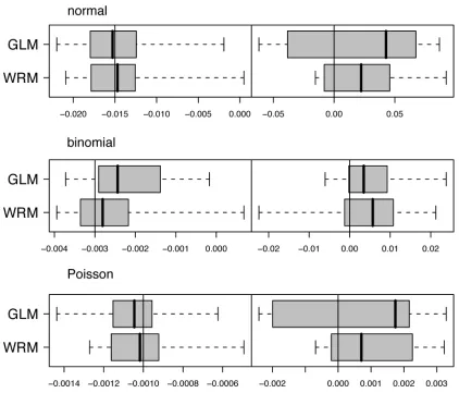
Table 1. Model quality: Spatial autocorrelation in the model residuals (given as global Moran’s I) and mean estimates for the coefficients ‘rain’ and ‘djungle’ (± 1 SE across the 10 simulations). True coefficient values are given in the first row for each distribution in italics. ***, * and ns refer to median significance levels of p < 0.001, 0.01 < p < 0.05 and p > 0.1, respectively, across the 10 realisations. GLM:
Generalized linear model, WRM: Wavelet-revised model.
Moran’s I Coefficients
‘rain’ ‘djungle’
Normal –0.015 0.0
GLM 0.016 ± 0.026 –0.0143 ± 0.0010*** 0.0220 ± 0.0508ns
WRM –0.001 ± 0.001 –0.0138 ± 0.0021*** 0.0250 ± 0.0285ns
Binomial –0.003 0.0
GLM 0.006 ± 0.011 –0.0022 ± 0.0003*** 0.0052 ± 0.0130ns
WRM –0.002 ± 0.000 –0.0025 ± 0.0011* 0.0034 ± 0.0154ns
Poisson –0.001 0.0
GLM 0.018 ± 0.024 –0.0010 ± 0.0000*** 0.0006 ± 0.0018ns
WRM –0.001 ± 0.001 –0.0010 ± 0.0002*** 0.0010 ± 0.0021ns
Fig. 2. Correlograms of one realisation for each of the three differ-ent distributions (normal, binomial, Poisson) and the methods compared.
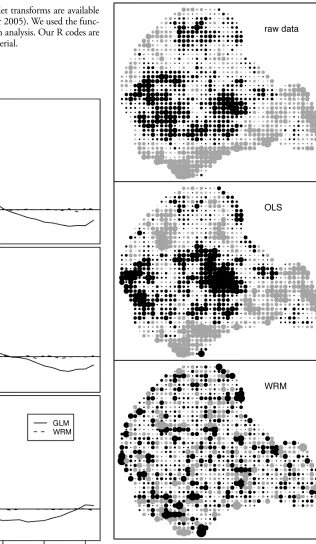
Fig. 3. Raw distributional data and residual maps for the different methods for one realisation of the data with normally distributed responses. On the residual maps, pixel sizes indicate sizes of resid-uals. The two colours black and grey represent the positive and negative signs of residuals, and areas of equal colour indicate au-tocorrelation. For WRM residuals the areas of equal colour are essentially reduced compared to OLS residuals.
sample size. The number of rows and columns must be dyadic (i.e.2n, where n is an integer). In general, one wishes
to analyze samples of arbitrary size though. For this reason data are padded with zeros until a quadratic matrix of re-quired size is reached (Bruce and Gao 1996).
For all subsequent analyses, our WRM method should be compared to the methods given in Dormann et al. (2007). Therefore, we present the results in the same way
Tricks and tips
The function mra.2d offers various wavelets. We used Haar wavelets. Because of the restriction to finite sets in discrete wavelet transforms it is necessary to give boundary treatment rules. Type periodic is implemented for bound-ary conditions in the software for the two-dimensional dis-crete wavelet transform. This causes a restriction on the
as it was done in that paper. Table 1 and Fig. 1–3 given here correspond to Table 2 and Fig. 1–3 in Dormann et al. (2007). For the purpose of comparison, the results of the non-spatial models OLS/GLM are given here as well.
Results
WRM models yield approximately the same values as ex-pected and as calculated by GLM for means and variances of the estimates ‘rain’ and ‘djungle’ (Fig. 1). However, only 10 data realizations were evaluated in each case of data with normally, binomially and Poisson-distributed re-sponses. Thus conclusions regarding model performance should be avoided here.
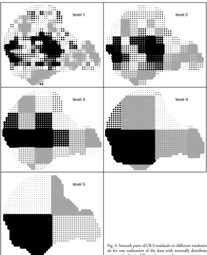
Our WRM model and the non-spatial model GLM differ obviously in the spatial signature of their residuals. Figure 2 shows that residual autocorrelation measured by Moran’s I is considerably reduced compared to GLM. Cor-responding values for Global Moran’s I are given in Table 1. WRM always performs better than GLM. Moreover, we present maps to determine whether there are any spatial patterns of regression residuals (Fig. 3). The maps show raw data y, OLS residuals and WRM residuals for a dataset with normally distributed responses. They demonstrate that WRM removes the clusters of positive or negative OLS residuals. WRM was carried out on level 1. Figure 4 shows patterns for smooth parts of OLS residuals at differ-ent resolutions. These smooth compondiffer-ents need to be re-moved for WRM residuals. Level 1 captures the smooth parts best describing the spatial autocorrelation structure in this dataset. The decorrelated WRM residuals (Fig. 3) can be imagined as the difference of OLS residuals (Fig. 3) and their smooth parts at the finest resolution, i.e. on level 1 (Fig. 4, top left).
Discussion
Dormann et al. (2007) presented an overview of different modelling approaches for multiple regressions displaying spatial autocorrelation. The authors state that the most flexible methods applicable to non-normal distributions are spatial GLMM, GEE and SEVM. Our new WRM method represents an alternative approach to obtain an approximately equal performance.
Carl and Kühn (2008) investigated the type I error con-trol of WRM in a more reliable analysis of 500 data realiza-tions per distribution. The results showed a better error calibration curve for WRM than for GLM. Furthermore, in comparing the above-mentioned models one has to consider the following facts:
(1) GLMM and GEE are useful to correct autocorrela-tion effects when the correlaautocorrela-tion structure is known as in our simulated datasets. WRM, however, provides a power-ful tool for removing autocorrelation without any prior
knowledge of the underlying correlation structure in lat-tice data. However, WRM requires comparably large sam-ples sizes whereas GEE may reach their limits with large sample sizes (Carl and Kühn 2007, Dormann et al. 2007). The methods may therefore be regarded as complementary.
(2) SEVM (and Bayesian) methods are very time-con-suming, whereas WRM is a computationally very fast and efficient procedure.
(3) Almost all methods assume spatial stationarity, i.e. spatial autocorrelation to be constant across the region, whereas WRM is a method that allows for spatial non-sta-tionarity. Moreover, WRM is able to detect anisotropic autocorrelation. This is true for at least such autocorrela-tion which acts differently in vertical, horizontal, and diag-onal direction.
Summarizing, this paper presented a wavelet-based method for regressions influenced by spatial autocorrela-tion. WRM is a good alternative to the methods described in Dormann et al. (2007), especially for large data-sets.
Acknowledgements – The authors acknowledge funding by the
European Union within the FP 6 Integrated Project ‘ALARM’ (GOCE-CT-2003-506675). Moreover, they acknowledge sup-port from the ‘Virtual Institute for Macroecology’, funded by the Helmholtz Association (VH-VI-153 Macroecology, Kühn et al. 2008). This contribution is based on the international workshop ‘Analysing spatial distribution data: principles, applications and software’ (GZ 4850/191/05) supported by the German Science Foundation (DFG).
References
Bruce, A. and Gao, H. Y. 1996. Applied wavelet analysis with S-plus. – Springer.
Carl, G. and Kühn, I. 2007. Analyzing spatial autocorrelation in species distributions using Gaussian and logit models. – Ecol. Modell. 207: 159–170.
Carl, G. and Kühn, I. 2008. Analyzing spatial ecological data using linear regression and wavelet analysis. – Stochastic En-viron. Res. Risk Assess. 22: 315–324.
Daubechies, I. 1992. Ten lectures on wavelets. CSBM-NSF Se-ries Application Mathematics. Vol. 61. – SIAM Publication. Dobson, A. J. 2002. An introduction to generalized linear
mod-els. – Chapman and Hall.
Dormann, C. F. et al. 2007. Methods to account for spatial auto-correlation in the analysis of species distributional data: a re-view. – Ecography 30: 609–628.
Hubbard, B. B. 1998. The world according to wavelets. – A. K. Peters.
Kissling, W. D. and Carl, G. 2008. Spatial autocorrelation and the selection of simultaneous autoregressive models. – Glo-bal Ecol. Biogeogr. 17: 59–71.
Kühn, I. 2007. Incorporating spatial autocorrelation may invert observed patterns. – Div. Distr. 13: 66–69.
Kühn, I. et al. 2008. Macroecology meets global change research. – Global Ecol. Biogeogr. 17: 3–4.
Myers, R. H. et al. 2002. Generalized linear models. – Wiley. Percival, D. B. and Walden, A. T. 2000. Wavelet methods for
time series analysis. – Cambridge Univ. Press.
R Development Core Team. 2005. R: a language and environ-ment for statistical computing. – R Found. Stat. Comp.