A New Method for Solving Fuzzy Assignment Problems

Annals of Pure and Applied Mathematics Vol. 1, No. 1, 2012, 69-83

ISSN: 2279-087X (P), 2279-0888(online) Published on 12 September 2012

www.researchmathsci.org

Annals of

A New Method for Solving Fuzzy Assignment Problems

P. Pandian1 _{and K. Kavitha}2

1 _{Department of Mathematics, School of Advanced Sciences,}

VIT University, Vellore-632 014, INDIA. E.mail: [email protected]

2 _{Department of Mathematics, School of Advanced Sciences,}

VIT University, Vellore-632 014, INDIA. E-mail: [email protected]

Received 3 September2012; accepted 11 September 2012

Abstract. A new method namely, parallel moving method is proposed to find an optimal solution to the fuzzy assignment problem considered in Lin and Wen [13]. We derive two theorems; one is related to an optimal solution to the fuzzy assignment problem and another is related to find an improved solution from the current solution to the fuzzy assignment problem. The parallel moving method provides an optimal solution to the fuzzy assignment problem in less number of iterations than the labeling algorithm [13]. A numerical example is given to demonstrate the procedure of the proposed method.

AMS Mathematics Subject Classification (2010): 90B80, 09C05, 90C10, 03E72 Keywords: Assignment problem, Fuzzy quantity, Fractional linear programming, Parallel moving method.

1. Introduction

The assignment problem (AP) is a special type of a transportation problem and a linear zero-one programming problem [11]. It is a one of the well-studied optimization problems in Management Science and has been widely applied in both manufacturing and service systems. The main object of the AP is to find an assignment schedule in a jobs assignment problem where n jobs are allocated to n workers and each worker receives exactly just one job such that the total assignment cost is minimum. The classical AP can also be written as a 0–1 integer programming problem as follows:

(P) Minimize n _{ij ij}

j n

i

x c z= ∑ ∑

70 n x i n

j ij

,..., 2 , 1 ; 1 1

= = ∑

= ;

n

x

j

n

i ij

,...,

2

,

1

;

1

1

=

=

∑

= ;

x_ij ={0,1}; i=1,2,...,n j=1,2,...,n

where x_ijis the decision variable, that is , ith worker in jth job and c_ijis the cost of the ith worker who are doing the jth job.

The AP introduced by Votaw and Orden [21] can be solved using the linear programming technique, the transportation algorithm or the Hungarian method developed by Kuhn [12]. The Hungarian method is recognized to be the first practical method for solving the standard assignment problem. Balinski and Gomory [2] introduced a labeling algorithm for solving the transportation and assignment problems. Ford and Fulkerson [9] introduced the models and algorithms in Flows in Networks which are used widely today in the fields of transportation systems, manufacturing, inventory planning, image processing, and Internet traffic. Aggarwal et al. [1] developed two algorithms for solving bottleneck assignment problems.

expressions. Shigeno et al. [19] proposed a solution procedure for the fractional assignment problem. Charnes and Cooper [7] introduced the variable transformation method for solving fractional programming model.

In this paper, we propose a new method namely, parallel moving method for finding an optimal solution to the FAP considered in Lin and Wen [13]. We construct two crisp APs from the given FAP. Using the optimal solutions of these two crisp APs, we develop the parallel moving method for solving the FAP. For ensuring the optimal solution to the FAP, we derive one theorem and for efficient section procedure of an improved solution from the current solution to the FAP, we derive another theorem. The proposed method provides an optimal solution to the FAP in less number of iterations than the labeling algorithm developed by Lin and Wen [13]. For computing the parameters in the parallel moving method, we follow the method of computation of the transportation algorithm. A numerical example is given to demonstrate the procedure of the proposed method. The parallel moving method enables the decision makers to evaluate the economical activities and make self satisfied managerial decisions when they are handling an AP having imprecise parameters.

2. Fuzzy Assignment Problem

We consider the following FAP studied in Lin and Wen[13].

72













=

≤

≤

−

−

=

≥

=

otherwise

:

0

1

;

:

)

(

)

(

1

;

:

(

_{) ij ij ij ij}

ij ij ij ij ij ij ij ij ij ij

ij

if

c

x

c

q

x

c

if

q

c

α

β

α

β

α

β

µ

We use the notation

α

_ij

,

β

_ij to denote c~_ij. The matrix [c~_ij] =

[

α

_ij

,

β

_ij ]. In addition, all the

α

_ij’s form the matrix [

α

_ij] and

β

_ij’s form the matrix [

β

_ij]. From the definition of c~_ij, any expense exceeding

β

_ijis useless since the quality (worker’s job performance or customer’s satisfaction) can no longer be increased at its upper limit

q

_ij.

Furthermore, let

c

~

_T denote the total cost, which related to the job performance of the manager, and numbers a and b are defined as the lower and upper bounds of total cost, respectively. We define the membership function of

c

~

_T

as the linear monotonically decreasing function and use the notation

a,

b

to denote fuzzy interval

c

~

_T. Numbers a and b are constants and are subjectively chosen by the manager. Using the idea from Werners [22], a number less than or equal to the minimum assignment of matrix [

α

_ij] as a and a number larger than or equal to the maximum assignment of matrix [

β

_ij] as b are taken. The membership function of

T

c

~

_{is given below:}













≥

≤

≤

−

−

≤

=

















∑

∑

=

= =

b

c

if

b

c

a

if

c

b

a

c

if

x

c

c

T T ij ij T T ij ij m j n i T

:

0

:

)

(

:

1

)

(

1

1

β

α

µ

µ

.

The main objective of the FAP is to find an assignment to the given FAP which minimize the total cost of workers and maximize the job performance of the manager.

The above FAP was modeled by Lin and Wen[13] as a 0-1 linear fractional programming problem as follows:

(FP) Maximize

n x i n j ij

,..., 2 , 1 ; 1 1

= =

∑

= (1)

n

x

j

n

i ij

,...,

2

,

1

;

1

1

=

=

∑

= (2)

x_ij ={0,1}; i=1,2,...,n j=1,2,...,n (3)

where

ij ij ij

ij _q

α

β

γ

= − .

We now, need the following result related to FAP which can be found in Lin and Wen [13].

Now, the linear programming model of the FAP, (LP) is given below: (LP) Maximize n _ijy_ij bt

j n

i

+ ∑

∑ −

= =1 1

α

subject to

n y_ij t i n j

,..., 2 , 1 , 1

= = ∑

=

;

yij t j n n

i

,..., 2 , 1 , 1

= = ∑

= ;

( ) 1 1

1

= − + ∑

∑

=

= ijyij b a t

n

j n

i

γ

;

t≥0, y_ij ≥0, i=1,2,...,n; j=1,2,...,n;

where

ij ij n

j n

i

x

a

b

t

γ

∑

∑

+

−

=

=

=1 1

1

and y_ij =tx_ij.

Now, the dual problem corresponding to (LP), (LD) is given below:

(LD) Minimize f

subject to

ui +vj +

α

ij + f

γ

ij ≥0, for all i and j

u vj b a f b

n

j i n

i∑ − ∑ + − ≥

−

=

=1 1 ( )

74

Result 2.1. Let X ={x_ij,i,j=1,2,...,n}be a feasible solution to FAP and }

n 1,2,..., j

i, ; , ,

{ =

= u v f

W _{i j} be the complementary solution for the dual

problem (LD) corresponding to Y ={y_ij,y_ij =tx_ij,i,j=1,2,...,n }. Then,

(i) if x_ij =1, that is, (i,j)th cell is allotted in FAP, then u_i+v_j +

α

_ij + f

γ

_ij =0 and

(ii) if u_i +v_j +

α

_ij + f

γ

_ij ≥0, for all non-allotted cells in the FAP, then }

,..., 2 , 1 , ,

{x i j n

X = _ij = is an optimal solution to FAP.

We now, construct two crisp APs (L) and (U) from the problem (FP) as follows:

(L) Minimize n _{ij ij} j

n

i x

z= ∑ ∑

α

=

=1 1

subject to (1), (2) and (3) are satisfied and

(U) Minimize n _{ij ij} j

n

i x

z= ∑ ∑

γ

=

=1 1

subject to (1), (2) and (3) are satisfied.

For easy computing and clear understanding , the parallel moving method will be applied directly on a table as that of classical transportation algorithm. Parameters corresponding to cell (i; j) are displayed in the Table 1..

Table 1.

3. The Parallel Moving Method

Now, we derive the following theorem which connects the solutions of the problem

(FP) and its deduction the problems (L) and (U) and is used in the parallel moving

method.

ij

α

δ

_ij

f

Theorem 3.1. Let

X

₀ be optimal solution to the problem (L) and

Y

₀ be optimal solution to the problem (U). Then,

X

₀ and

Y

₀ are feasible solution to the fuzzy assignment problem and

≤

)

(

)

(

0 0

X

Q

X

P

Max.

f

(X

)

≤

)

(

)

(

0 0

Y

Q

X

P

and

≤

)

(

)

(

0 0

Y

Q

Y

P

Max.

f

(

X

)

≤

)

(

)

(

0 0

Y

Q

X

P

where n _{ij ij}

j n i x b X

P = − ∑ ∑

α

=

=1 1

)

( and n _{ij ij}

j n i x a b X

Q = − + ∑ ∑

γ

=

=1 1

)

( If

X

₀ and

Y

₀

are the same, then

X

₀ is an optimal solution to the fuzzy assignment problem

and Max.

f

(

X

)

=

.

)

(

)

(

0 0

X

Q

X

P

Proof: Now, since

X

₀ is optimal solution to the problem (L), then

X

₀ is optimal solution to the problem (N) where

(N) Maximize n _{ij ij}

j n

i

x b

P= − ∑ ∑

α

=

=1 1

subject to (1), (2) and (3) are satisfied.

Now, since

Y

₀ is optimal solution to the problem (U), then

Y

₀ is optimal solution to the problem (D) where

(D) Minimize n _{ij ij}

j n i x a b

Q= − + ∑ ∑

γ

=

=1 1

subject to (1), (2) and (3) are satisfied.

Now,

(

)

)

(

)

(

1 1 1

1

_f

_X

x

a

b

x

b

X

Q

X

P

ij ij n j m i ij ij n j m i

₌

∑

∑

+

−

∑

∑

−

=

= = = =

γ

α

Let

X

be a feasible solution to the problem (FP).

Clearly,

X

is a feasible solution to the problems (N) and (D). Then, we have

)

(

)

(

X

P

X

₀

P

≤

and

Q

(

X

)

≥

Q

(

Y

₀

)

.

Since

Q

(

X

)

>

0

, we have

)

(

)

(

)

(

)

(

0 0

Y

Q

X

P

X

Q

X

P

_≤

.

This implies that Max.

76 Therefore, ) ( ) ( ) ( . 0 0 Y Q X P X f

Max ≤ . (4)

Now, since

X

₀ and

Y

₀ are feasible solutions to the problem (FP), we have

)

(

.

)

(

X

₀

Max

f

X

f

≤

and

f

(

Y

₀

)

≤

Max

.

f

(

X

)

. (5)

Now, from (4) and (5), we have

≤

)

(

)

(

0 0

X

Q

X

P

Max.

f

(

X

)

≤

)

(

)

(

0 0

Y

Q

X

P

and

≤

)

(

)

(

0 0

Y

Q

Y

P

Max.

f

(

X

)

≤

)

(

)

(

0 0

Y

Q

X

P

. (6)

Now, given that

X

₀ and

Y

₀ are the same. From (6), we have

≤

)

(

)

(

0 0

X

Q

X

P

Max.

f

(

X

)

≤

)

(

)

(

0 0

X

Q

X

P

and

≤

)

(

)

(

0 0

X

Q

X

P

Max.

f

(

X

)

≤

)

(

)

(

0 0

X

Q

X

P

This implies that, Max.

f

(

X

)

=

(

).

)

(

)

(

0 0

0

_f

_X

X

Q

X

P

₌

Therefore,

X

₀ is an optimal solution to the problem (FP) and

Max.

f

(

X

)

=

.

)

(

)

(

0 0

X

Q

X

P

Hence the theorem.

Now, we prove the following theorem corresponding to the selection of an improved solution from the current solution of the problem (FP) which is used in the proposed method.

Theorem 3.2. Let

X

₀

=

{

x

_ijo

,

i

,

j

=

1

,

2

,...,

n

}

_{be a solution to the problem (FP) in}

which

(

p

,

r

)

and

(

q

,

s

)

are two allotted cells, that is , o

=

o

=

1

qs pr

x

x

and

)

,

(

p

s

and

(

q

,

r

)

are non-allotted cells, that is , o

=

o

=

0

qr ps

x

x

such that

}

,...,

2

,

1

,

,

{

1

1

x

i

j

n

X

=

_ij

=

where 1

=

o

=

1

,

ij ij

x

x

for all

(

i

,

j

)

≠

(

p

,

r

)

and

(

q

,

s

)

Proof: Now, we have, ij ij ij ij x a b x b X f f

γ

α

∑ ∑ + − ∑ ∑ − = = ) ( )

( where

}. ,..., 2 , 1 , ,

{x i i n

X = _ij =

Now, ij ij ij ij x a b x b X f f 0 0 0 0 ) ( ) (

γ

α

∑ ∑ + − ∑ ∑ − =

= and

ij ij ij ij x a b x b X f f 1 1 1 1 ) ( ) (

γ

α

∑ ∑ + − ∑ ∑ − = = . Now, ij ij ij ij x a b x b f 1 1 1 ) (

γ

α

∑ ∑ + − ∑ ∑ − = ) ( ) ( 0 0 qs pr qr ps ij ij qs pr qr ps ij ij x a b x b

γ

γ

γ

γ

γ

α

α

α

α

α

− − + + ∑ ∑ + − + + − − ∑ ∑ − =

Since (

γ

_pr +

γ

_qs)−(

γ

_ps +

γ

_qr)≤0, we have

78 ij ij ij ij x a b x b 0 0 ) (

γ

α

∑ ∑ + − ∑ ∑ − = ij ij qr ps qs pr

x

a

b

)

0

(

)

(

)

(

γ

α

α

α

α

∑

∑

+

−

+

−

+

+

=

f

₀

ij ij qr ps qs pr

x

a

b

)

0

(

)

(

)

(

γ

α

α

α

α

∑

∑

+

−

+

−

+

+

Since (b−a)+∑ ∑

γ

ijx0ij >0 and (

α

pr +

α

qs)−(

α

ps +

α

qr)≥0, we can

conclude that

0

0

1

−

f

≥

f

.

Hence the theorem.

Now, we extend the result of the Theorem 3.2. to a set of allotted cells to another set of non-allotted cells of the solution of the problem (FP). .

Theorem 3.3. Let

X

₀

=

{

x

_ijo

,

i

,

j

=

1

,

2

,...,

n

}

_{be a solution to the problem (FP) in} which

E = (p₁,r₁), (p₂,r₂), …,

(

p

_t

,

r

_t

)

; o₁₁

=

_L

=

o

=

1

t r t p r p

x

x

} and

D = {(q₁,s₁), (q₂,s₂),…,

(

q

_t

,

s

_t

)

; o₁₁

=

_L

=

o

=

0

t s t q s q

x

x

}

)

and

2

(

t

≥

t

≤

n

,

are subsets of

X

₀ such that

X

₁

=

{

x

1_ij

,

i

,

j

=

1

,

2

,...,

n

}

where

1

=

o

=

1

,

ij ij

x

x

for all

(

i

,

j

)

≠

(

p

_a

,

r

_a

)

and

(

q

_a

,

s

_a

)

(

a

=

1

,

2

,...,

t

);

x1 1(a 1,2,3,..,t) a

s a

p = = ; x1q_br_b+1 =1(b=1,2,...,t−1) and x1q_tr₁ =1, is a solution to the problem (FP). Then,

f

(

X

₁

)

≥

f

(

X

₀

)

provided

0

)

(

)

(

)

(

1 _{1 1}

1

1

+

−

∑

+

−

+

≤

∑

− ₊

=

= pasa qara ptst qtr

t a a s a q a r a p t

a

γ

γ

γ

γ

γ

γ

and

0

)

(

)

(

)

(

1 _{1 1}

1

1

+

−

∑

+

−

+

≥

∑

− ₊

=

= pasa qara ptst qtr

t a a s a q a r a p t

a

α

α

α

α

α

α

.

Proof: It is similar to the proof of the Theorem 3.2.

We now, propose a new method namely, parallel moving method for solving the problem (FP).

The parallel moving method proceeds as follows.

Step 1: Construct the APs (L) and (U) from the given FAP. Then, solve them by the Hungarian method. Say

X

₀ is an optimal solution to the problem (L) and

Y

₀ is an optimal solution to the problem (U).

Step 2: If

X

₀ =

Y

₀, then

X

₀ is an optimal solution to the given FAP by the Theorem 3.1. and go to the Step 7. . If not, go to the Step 3..

Step 3: Fix

U

₀ where

U

₀

=

X

₀ or

Y

₀ as an initial solution to the given FAP. Then, compute the value of

f

(

U

₀

)

,

f

₀.

Step 4: Compute the dual variables ( MODI indices) u_i and v_j for all i and j using the relation u_i +v_j +

α

_ij + f₀

γ

_ij =0, for allotted cells by taking u_i =0, for all i.

Step 5: Construct MODI index table for the initial solution,

U

₀to the FSP. Then, compute

δ

_ij =u_i+v_j+

α

_ij + f₀

γ

_ij for all non-allotted cells. If

δ

_ij ≥0, for all non-allotted cells, go to the Step 7.. If not, go to the Step 6..

Step 6: Find a cell having the most negative value of

δ

_ij. Say

(

p

,

s

)

. Then,

(a) if the assignments of

p

and s in the initial solution

U

₀ are

(

p

,

r

)

and

(

q

,

s

)

and

if (

γ

_pr +

γ

_qs)−(

γ

_ps +

γ

_qr)≤0 and (

α

_pr +

α

_qs)−(

α

_ps+

α

_qr)≥0, assign

)

,

(

p

s

and

(

q

,

r

)

(see Table 2.) and obtain an improve solution

}

,

(

),

,

{(

)})

,

(

),

,

{(

(

₀

1

U

p

r

q

s

p

s

q

r

U

=

−

∪

by the Theorem 3.2.. Then, go to the

Step 2. for next iteration.

If the one of the conditions “(

γ

_pr +

γ

_qs)−(

γ

_ps +

γ

_qr)≤0 and 0

) (

)

(

α

_pr +

α

_qs −

α

_ps+

α

_qr ≥ ” is not satisfied, go to Step 6.(b).

(b) Find a cell in the qth row , say

(

q

,

t

)

which satisfies the conditions 0

) (

)

(

γ

_pr +

γ

_qs +

γ

_zt −

γ

_ps +

γ

_qt +

γ

_zr ≤ and 0 ) (

)

(

α

_pr +

α

_qs +

α

_zt −

α

_ps +

α

_qt+

α

_zr ≥ where

(

z

,

t

)

is the assignment of t in the initial solution

U

₀, assign

(

p

,

s

)

,

(

q

,

t

)

and

(

z

,

r

)

( see the Table 3.) and obtain an improve solution

)}

,

(

),

,

(

),

,

{(

)})

,

(

),

,

(

),

,

{(

(

₀

1

U

p

r

q

s

z

t

p

s

q

t

z

r

80

If the one of the conditions “(

γ

_pr +

γ

_qs +

γ

_zt)−(

γ

_ps+

γ

_qt +

γ

_zr)≤0 and 0

) (

)

(

α

_pr +

α

_qs +

α

_zt −

α

_ps +

α

_qt+

α

_zr ≥ ” is not satisfied, go to Step 6.(c).

(c) Continue for finding an assignment to the rth column as like as in the Step 6(b). After finite number of steps, an improve solution is obtained. Then, go to the Step 2. for the next iteration.

Step 7: The current solution is an optimal solution to the given FAP . We stop the computation process. The current value of

f

is the maximum value of

f

.

Table 2. Table 3.

( Marks X denote current allotments and Marks # denote new allotments )

Now, the parallel moving method is illustrated with the help of the following numerical example.

Example 3.1. Consider the following 3×3 fuzzy assignment problem whose fuzzy cost matrix, [c~_ij]and quality matrix, [q_ij]are given below:

          = ] 12 , 6 [ ] 8 , 4 [ ] 10 , 7 [ ] 15 , 7 [ ] 14 , 6 [ ] 13 , 4 [ ] 6 , 2 [ ] 12 , 3 [ ] 13 , 4 [ ] ~

[c_ij and

          = 6 . 0 8 . 0 6 . 0 8 . 0 8 . 0 9 . 0 8 . 0 6 . 0 9 . 0 ]

[q_ij .

Then, we obtain the following matrices:

          = 6 4 7 7 6 4 2 3 4 ]

[

α

_ij ;

          = 12 8 10 15 14 13 6 12 13 ]

[

β

_ij and

          = 10 5 5 10 10 10 5 15 10 ] [

γ

_ij

Now, by the Hungarian method, we obtain that the optimal solution to (L) is (1,3), (2,1) and (3,2) and the optimal solution to (U) are (1,3) (2,1) and (3,2) and (1,3) , (2,2) and (3,1).

R … s

P X … #

M

_M

_M

_M

Q # … X

r … t … s

P X … … #

M

_M

_M

M

_M

_M

Z # X

M

_M

_M

M

_M

_M

Now, the common solution is (1,3), (2,1) and (3,2).

Now, the

(

α

,

γ

)

−

table corresponding to FAP is given below: 4

10 3

15 2

5 4

10 6

10 7

10 7

5 4

5 6

10

Case (i) Initial solution: (1,3), (2,1) and (3,2).

Now, the value of

f

for the above allotment =0.6. Hence,

f

=

0

.

6

Now, by the Theorem 1. and the assignment (1,3), (2,1) and (3,2) is the common solution to (L) and (U), the optimal allotment is (1,3), (2,1) and (3,2) and the optimal value of

f

=

0

.

6

.

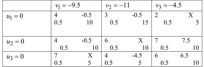
Case (ii) Initial solution: (1,3), (2,2) and (3,1).

Now, the value of

f

for the above allotment =0.5. Hence,

f

=

0

.

5

Take

u

_i

=

0

,

for all i.

Now, v_j =−

α

_ij − f

γ

_ij, for all allotted cells.

Now,

v

₁

=

−

α

₃₁

−

f

γ

₁₁= −9.5 ; v₂ =−

α

₂₂− f

γ

₂₂=

−

11

and 13

13

3

α

f

γ

v

=

−

−

=−4.5.

To check the optimality- MODI index table: 5 . 9 1=−

v v₂ =−11

v

₃

=

−

4

.

5

0 1=

u 4 -0.5

0.5 10

3 -0.5 0.5 15

2 X 0.5 5

0 2 =

u 4 -0.5

0.5 10

6 X 0.5 10

7 7.5 0.5 10

0

3

=

u

7 X

0.5 5

4 -4.5 0.5 5

6 6.5 0.5 10

The cell corresponding to most negative of

δ

_ij for all non-allotted cells is (3,2). Since we have the assignment (2,2) and (3,1) and

(

γ

₂₂

+

γ

₃₁

)

−

(

γ

₃₂

+

γ

₂₁

)

=

0

;

0

5

)

(

)

82

Now, the solution to the fuzzy assignment problem is (1,3), (2,1) and (3,2), and the value of

f

for the new allotment is 0.6. Hence ,

f

=

0

.

6

Since the assignment is optimal assignment to (L) and (U), the assignment is optimal to FAP by the Theorem 1.. Therefore, the optimal value of

f

= 0.6.

Remark 3.1: In Lin and Wen [13], the Example 3.1. was solved by LW algorithm in 4 iterations , but by the parallel moving method, we solve it at most one iteration.

4. Conclusion

Assignment problem is one of the most important problem in decision-making. In many real life applications, costs of AP are not deterministic numbers. The FAP is more realistic than the AP because most real environments are uncertain. In recent years, many researchers have begun to investigate AP and its variants under fuzzy environments. In Lin and Wen [13], a fuzzy assignment problem in which the cost of each job, depending on the quality, is not a deterministic number, was studied and solved it by the labeling method [13]. In this paper, we propose a new method namely, parallel moving method for solving the fuzzy AP problem considered in Lin and Wen [13]. From the Example 3.1., we can observe that our proposed method performs satisfactorily and is better than labeling algorithm [13]. In near future, we extend our study to the sensitivity analysis in the fuzzy assignment problem considered in Lin and Wen [13].

Acknowledgements

The authors thank the anonymous referee and the Chief-Editor for their valuable comments and suggestions, which were very helpful in improving the presentation of this paper.

REFERENCES

1. V. Aggarwal, V.G. Tikekar and L-F. Hsu, Bottleneck assignment problems under categorization, Computers and Operations Research, 13 (1986) 11– 26.

2. M.L.Balinski and R.E. Gomory, A primal method for the assignment and transportation problems, Management Science, 10 (1967 ) 578-593.

3. R.E. Bellman and L.A. Zadeh, Decision-making in a fuzzy environment, Management Science, 17B (1970) 141–164.

4. S. Chanas, W. Kolodziejczyk and A. Machaj, A fuzzy approach to the

transportation problem, Fuzzy Sets and Systems, 13 (1984) 211–221.

5. S. Chanas and D. Kuchta, A concept of the optimal solution of the

6. S. Chanas and D. Kuchta, Fuzzy integer transportation problem, Fuzzy Sets and Systems, 98 (1998) 291–298.

7. Charnes and W.W. Cooper, Programming with linear fractionals, Naval Res. Logist. Quart., 9 (1962) 181–186.

8. M.S. Chen, On a fuzzy assignment problem, Tamkang J., 22 (1985) 407–411. 9. L.R. Ford, Jr. and D.R. Fulkerson, Flows in Networks, Princeton University

Press, Princeton, NJ, 1966.

10. Y.Feng and L.Yang, A two objective fuzzy k-cardinality assignment problem, Journal of Computational and Applied Mathematics, 1(2006) 233-244

11. T. Koltai and T. Terlaky, The difference between the managerial and mathematical interpretation of sensitivity analysis results in linear programming, International Journal of Production Economics, 65 (2000) 257-274.

12. H.W. Kuhn, The Hungarian method for the assignment and transportation problems, Naval Research Logistics Quarterly, 2 (1955) 83–97.

13. C.J. Lin and U.P. Wen, The labeling algorithm for the fuzzy assignment problem, Fuzzy Sets and Systems, 142 (2004) 373–391.

14. Long-sheng Huang and Guang-hui Xu , Solution of assignment problem of restriction of qualification, Operations Research and Management Science, 14 (2005) 28-31.

15. Michéal ÓhÉigeartaigh, A fuzzy transportation algorithm, Fuzzy Sets and Systems, 8 (1982) 235–243.

16. P. Pandian and G. Natarajan, An appropriate method for real life fuzzy transportation problems, International Journal of Information Sciences and Applications, 2 (2010) 75-82.

17. P. Pandian and G. Natarajan, A new algorithm for finding a fuzzy optimal solution for fuzzy transportation problems, Applied Mathematical Sciences, 4 (2010) 79 – 90.

18. M.Sakawa, I.Nishizaki and Y.Ucmura, Interactive fuzzy programming for two-level linear and linear fractional production and assignment problems: a case study, European Journal of Operational Research, 135 (2001) 142-157.

19. M. Shigeno, Y. Saruwatari and T. Matsui, An algorithm for fractional assignment problems, Discrete Applied Mathematics, 56 (1995) 333–343. 20. M. Tada and H. Ishii, An integer fuzzy transportation problem, Comput. Math.

Appl., 31 (1996) 71–87.

21. D.F. Votaw and A. Orden, The personal assignment problem, Symposium on linear inqualities and programming, Project SCOOP 10, US Air Force, Washington, 1952, 155-163.