Numerical Solution of Fuzzy Differential Equation by Sixth Order Runge-Kutta Method

Vol. 7, No. 1, 2015, 35-42

ISSN: 2320 –3242 (P), 2320 –3250 (online) Published on 22 January 2015

www.researchmathsci.org

35

International Journal of

Numerical Solution of Fuzzy Differential Equation by

Sixth Order Runge-Kutta Method

S. Rubanraj1 and P. Rajkumar2

1

Department of Mathematics, St. Joseph’s College (Autonomous), Trichy, India Email:[email protected]

2

Department of Mathematics, St. Joseph’s College (Autonomous), Trichy, India Email: [email protected]

Corresponding Author

Received 3 November 2014; accepted 4 December 2014

Abstract. In this paper, in order to increase the order of the accuracy of the solution, we

propose a method of computing approximate solution of the fuzzy differential equation with initial conditions. The sixth order Runge-Kutta method is discussed in detail followed by a complete error analysis.

Keywords: Fuzzy differential equations, numerical solution, sixth order Runge-kutta

method

AMS Mathematics Subject Classification (2010): 34A07 1. Introduction

The topic of fuzzy differential equation has been rapidly growing in recent years. The concept of fuzzy derivatives was first introduced by Chang and Zadeh [7]; it was followed up by Dubois and Prade [8] who used the extension principle in their approach. Puri and Ralesec [16] and Goetschel and Voxman [10] contributed towards the differential of fuzzy functions. The fuzzy differential equation and initial value problems were extensively studied by Kaleva [11, 12] and by Seikkala [17]. Numerical solution of fuzzy differential equations has been introduced by Ma, Friedman, Kandel [14] through Euler method and by Abbasbandy and Allahviranloo [2] by Taylor method. Runge-Kutta methods have also been studied by authors [3, 15]. This paper is organized as follows: In Section 2, we give some basic definitions and results on fuzzy numbers and fuzzy derivatives. Section 3 contains the definition of fuzzy Cauchy problem with initial conditions. In Section 4 we propose the sixth order Runge-Kutta method to solve the fuzzy differential equation with initial condition. The proposed method is illustrated and solved the numerical example in section 5. Also the result of the approximation solution by Runge-Kutta sixth order method is compared with Euler’s method and Runge-Kutta fourth order method.

2. Preliminaries

36 We assume that

1. f(t, y(t)) is defined and continuous in the strip t0≤ t ≤ b, -∞<y<∞ with t0 and b are

finite.

2. There exists a constant L such that for any t in [t0, b] and any two numbers y and y *

( )

( )

* *

,

,y f t y Ly y t

f − ≤ −

These conditions are sufficient to prove that ∃on [t0, b] a unique continuous differentiable

function y(t) satisfying (2.1)

The basis of all Runge-Kutta methods is to express the difference between the value of y at tn+1 and tn as

∑

= + − =

m

i i i n

n y wk

y

0

1 ; where wi are constants and ki = hf(tn+aih, yn +

∑

−

=

1

1

i

j j ijk

c )

Most efforts to increase the order of accuracy of the Runge-Kutta methods have been accomplished by increasing the number of Taylor’s series terms used and thus the number of functional evaluations required [6]. The method proposed by Goeken and Johnson. O [9] introduces new terms involving higher order derivatives of ‘f’ in the Runge-Kutta ki terms (i > 1) to obtain a higher order of accuracy without a corresponding

increase in evaluations of f, but with the addition of evaluations of f1. Consider y(tn+1) = y(tn) + w1k1 + w2k2 + w3k3 + w4k4 + w5k5 + w6k6 + w7k7

where

k1 = hf(tn, y(tn))

k2 = hf(tn+c2h, y(tn)+a21k1)

k3 = hf(tn+c3h, y(tn)+a31k1+a32k2)

k4 = hf(tn+c4h, y(tn)+a41k1+a42k2+a43k3)

k5 =hf(tn+c5h,y(tn)+a51k1+a52k2+a53k3+a54k4)

k6 =hf(tn+c6h,y(tn)+a61k1+a62k2+a63k3+a64k4+a65k5+a66k6)

k7 = h f(tn+c7h,y(tn)+a71k1+a72k2+a73k3+a74k4+ a75k5+a76k6 + a77k7) (2.2)

Utilizing the Taylor’s series expansion techniques, Runge-Kutta method of order sixth is

given by yn+1 = yn +

180

9 49 49 64

9k₁+ k₃+ k₅+ k₆+ k₇

where

k1 = hf(tn, y(tn))

k2 = hf(tn+ vh, y(tn)+ vk1)

k3 = hf(tn+

2 h _{, y(t}

n)+ ((4v – 1)k1 + k2)/(8v))

k4 = hf(tn+

3 2 h _{, y(t}

n)+((10v – 2)k1 + 2k2 + 8vk3)/(27v))

k5 = hf(tn+(7+4.582576)

14 h _,y(t

n)+(-((77v–56)+(17v–8)4.582576)k1–8(7+4.582576)k2

+ 48(7+4.582576)vk3 – 3(21+4.582576)vk4)/(392v)

k6 =hf(tn+(7 - 4.582576)

14

h _{,y(tn)+(-5((287v–56) - (59v–8)4.582576)k1–40(7-4.582576)k2}

+ 320(4.582576)vk3+ 3(21-121(4.582576))vk4 + 392(6-4.582576)vk5) /(1960v)

k7 = hf(tn+ h,y(tn)+(15((30v – 8) - 7v(4.582576))k1+120k2– 40(5 + 7(4.582576))vk3

37

Definition 2.1. A fuzzy number u is a fuzzy subset of ℜ i.e., u: ℜ→[0, 1] satisfying the following conditions.

i). u is normal, i.e. ∃x0∈ℜ∋u(x0) = 1

ii). u is a convex fuzzy set

i.e.) u(tx + (1-t)y) ≥ min{u(x), u(y)}, ∀ t ∈ [0, 1] and x, y ∈ℜ iii).u is upper semi continuous on ℜ

iv).

{

x∈R,u

( )

x >0

}

is compact

The set E is the family of fuzzy numbers and arbitrary fuzzy number is represented by an ordered pair of functions

(

u

( ) ( )

r ,ur

)

, 0 ≤ r ≤ 1 that satisfies the following requirements.

1. u

( )

r is a bounded left continuous non-decreasing function over [0, 1] with respect to any ‘r’.

2. u

( )

r is a bounded right continuous non-increasing function over [0, 1] with respect to any ‘r’.

3. u

( )

r ≤u

( )

r , 0≤r ≤ 1, r-level cut is [u]r = {x/u(x) ≥ r}, 0 ≤ r ≤ 1 is closed

&bounded interval denoted by [u]r=

[

u

( ) ( )

r ,ur

]

and clearly [u]0 = {x/u(x)>0} is

compact.

Definition 2.2. A triangular fuzzy number u is a fuzzy set in E that is characterized by an ordered triple (ul,uc,ur)∈R

3

with ul<uc<ur such that [u]0 = [ul : ur] and [u]1 = [uc]. The

membership function of the triangular fuzzy number u is given by

( )

  

  

 

≤ ≤ −

− =

≤ ≤ −

−

=

r c

c r

r

c c l

l c

l

u x u u u

x u

u x

u x u u u

u x

x u

, 1

,

. . . (2.4)

and we will have

i). u > 0 if ul> 0

ii). u ≥ 0 if ul≥ 0

iii).u < 0 if uc< 0

iv).u ≤ 0 if uc≤ 0

Let I be a real interval. A mapping y: I → E is called a fuzzy process and its α - level set is denoted by

[ ]

y

( )

t _α=

[

y

( ) ( )

t,y,yt,y

]

, t ∈ I, 0 <α≤ I.

The Seikkala derivative y(t) of a fuzzy process is defined by

[ ]

y1

( )

t _α=

[

y1

( ) ( )

t,y,y1t,y

]

, t ∈ I, 0 <α≤ I provided the equation defines fuzzy number as in [12].For u, v ∈ E and λ∈ℜ, the u + v and the product λu can be defined by [u + v]α = [u]α + [v]α and [λu]α = λ[u]α, where α∈ [0, 1] and [u]α + [v]α means the addition of two intervals of ℜ and λ[u]α means the product between a scalar λ and a subset of ℜ.

Arithmetic operations of arbitrary fuzzy numbers u =

(

u

( ) ( )

r,ur

)

and v =

(

v

( ) ( )

r ,v r

)

, λ∈ℜ can be defined as

i). u = v if u

( ) ( )

r =vr and u

( ) ( )

r =vr

38 iii).u - v =

(

u

( ) ( ) ( ) ( )

r −vr ,ur −vr

)

iv).λu =

(

λu

( ) ( )

r,λur

)

if λ≥ 0 =

(

λu

( ) ( )

r,λu r

)

if λ< 0

3. Fuzzy Cauchy problem

Consider the fuzzy initial value problem

( ) (

t f t,y(t)

)

y′ = , 0≤ t ≤T, y(0) = y0 (3.1)

where f is a continuous mapping from ℜ+ x ℜ→ℜ and y0∈ E with r-level sets [y0]r =

( ) ( )

[

y0:r,y0:r

]

, r ∈ [0, 1]. The extension principle of Zadeh leads to the following definition of f(t, y),where y = y(t) is a fuzzy number.

f(t, y)(s)=sup{y(τ)\s=f(t, τ)}, s ∈ℜ

⇒

[

f

( )

t,y

]

_r=

[

f

(

t,y:r

) (

,f t,y:r

)

]

, r∈[0, 1] It follows that

(

t y r

)

{

f

( )

tu u

[

y

( ) ( )

r yr

]

}

f , : =min , \ ∈ , and f

(

t,y:r

)

=max

{

f

( )

t,u \u∈

[

y

( ) ( )

r,yr

]

}

. . . (3.2)

Theorem 3.1. Let f satisfy f

( )

t,v −f

( )

t,v ≤g

(

t,v−v

)

, t ≥ 0 and v,v ∈ℜ, (3.3)

where g : ℜ+ x ℜ+→ℜ+ is a continuous mapping such that r → g(t, r) is non-decreasing

and the initial value problem u1(t) = g(t, u(t)), u(0) = u0 (3.4)

has a solution on ℜ+for u0> 0 and that u(t)≡ 0 is the only solution of (3.4) for u0 = 0. Then

the fuzzy initial value problem (3.1) has a unique solution.

Proof: See [17].

3.1. Sixth order Runge–Kutta method

Let the exact solution of the given equation [y(t)]r =

[

y

( ) ( )

t:r,yt:r

]

is approximated by

some [y(t)]r =

[

y

( ) ( )

t:r,yt:r

]

and we define

(

) ( )

∑

=

+ − =

7

1

1: :

i i i n

n r yt r wk

t

y and

(

) (

)

∑

=

+ − =

7

1

1: :

i i i n

n r y t r wk

t y

where wi’s are constants,

( )

(

)

[

k_i t,yt,r

]

_r =

[

k_i

(

t,y

( )

t,r

)

,k_i

(

t,y

( )

t,r

)

]

where i = 1, 2, 3, 4, 5, 6, 7

( )

(

t yt r

)

hf

(

t y

(

t r

)

)

k₁ , : = _n, _n:

( )

(

t yt r

)

hf

(

t y

( )

t r

)

k₁ , : = _n, _n:

( )

(

)

(

)



  

 

+ +

= 1

2 , :

2 :

,yt r hf t h yt r vk t

k _{n n}

( )

(

)

(

)



  

 

+ +

= 1

2 , :

2 :

,yt r hf t h yt r vk t

k _{n n}

( )

(

)

(

) (

(

)

)



  

 

+ − + +

=hf t h yt r v k k v

r t y t

k _n , _n: 4 1 /8

2 :

, _{1 2}

3

( )

(

)

( ) (

(

)

)



  

 

+ − + +

=hf t h yt r v k k v

r t y t

k n , n: 4 1 /8

2 :

, 1 2

39

( )

(

)

(

) (

(

)

)

      + + − + +

=hf t h yt r v k k vk v

r t y t

k n , n: 10 2 2 8 /27

3 2 :

, 1 2 3

4

( )

(

)

( ) (

(

)

)

      + + − + +

=hf t h yt r v k k vk v

r t y t

k n , n: 10 2 2 8 /27

3 2 :

, 1 2 3

4

( )

(

)

(

)

( )

(

(

(

) (

)

)

(

)

)

(

)

                       + − + + + − − + − − + + + = v k v k v k k v v r t y h t hf r t y t

k _{n n} /392

582576 . 4 21 3 582576 . 4 7 48 582576 . 4 7 8 582576 . 4 8 17 56 77 : , 14 582576 . 4 7 : , 4 3 2 1 5

( )

(

)

(

)

( )

(

(

(

) (

)

)

(

)

)

(

)

                       + − + + + − − + − − + + + = v k v k v k k v v r t y h t hf r t y t

k _{n n} /392

582576 . 4 21 3 582576 . 4 7 48 582576 . 4 7 8 582576 . 4 8 17 56 77 : , 14 582576 . 4 7 : , 4 3 2 1 5 ( ) ( ) ( ) ( ) ( ) ( ) ( ) ( ) ( ) ( ) ( ) ( ( ))                        − + − + + − − − − − − + − + = v k v k v k v k k v v r t y h t hf r t y t

k n n /1960

582576 . 4 6 392 582576 . 4 121 21 3 582576 . 4 320 582576 . 4 7 40 582576 . 4 8 59 56 287 5 : , 14 582576 . 4 7 : , 5 4 3 2 1 6 ( ) ( ) ( ) ( ) ( ) ( ) ( ) ( ) ( ) ( ) ( ) ( ( ))                        − + − + + − − − − − − + − + = v k v k v k v k k v v r t y h t hf r t y t

k _{n n} /1960

582576 . 4 6 392 582576 . 4 121 21 3 582576 . 4 320 582576 . 4 7 40 582576 . 4 8 59 56 287 5 : , 14 582576 . 4 7 : , 5 4 3 2 1 6

( )

(

)

( )

(

(

(

(

) (

)

)

)

)

(

(

(

(

)

)

)

)

(

)

(

)

                       + + − − + + + − + − + + = v k v k v k v k v k k v v r t y h t hf r t y t

k _{n n} /180

582576 . 4 7 70 582576 . 4 9 49 14 582576 . 4 3 2 63 582576 . 4 7 5 40 120 582576 . 4 7 8 30 15 : , : , 6 5 4 3 2 1 7

( )

(

)

( )

(

(

(

(

) (

)

)

)

)

(

(

(

)

)

(

)

)

(

)

(

)

                       + + − − + + + − + − − + + = v k v k v k v k v k k v v r t y h t hf r t y t

k n n /180

582576 . 4 7 70 582576 . 4 9 49 14 582576 . 4 3 2 63 582576 . 4 7 5 40 120 582576 . 4 7 8 30 15 : , : , 6 5 4 3 2 1 7 (4.1)

( )

(

t yt r

)

k

(

t y

( )

t r

)

k

(

t y

( )

t r

)

k

(

t y

( )

t r

)

k

(

t y

( )

t r

)

k

(

t y

( )

t r

)

F , : =9₁ , : +64 ₃ , : +49 ₅ , : +49 ₆ , : +9 ₇ , :

( )

(

t yt r

)

k

(

t y

( )

t r

)

k

(

t y

( )

t r

)

k

(

t y

( )

t r

)

k

(

t y

( )

t r

)

k

(

t y

( )

t r

)

G , :

7 9 : , 6 49 : , 5 49 : , 3 64 : , 1 9 : , = + + + +

The exact and approximate solution at tn, 0 ≤ n ≤N are denoted by

[Y(tn)]r =

[

Y

(

t_n:r

) (

,Y t_n:r

)

]

and [y(tn)]r =

[

y

(

t_n:r

) (

,y t_n:r

)

]

respectively.

The solution calculated by grid points at a = t0≤ t1≤ t2≤ . . . ≤tN = b and

h =

N a b− _{= t}

n+1 – tn. Therefore we have

(

t r

) (

Y t r

)

F

[

t Y

(

t r

)

]

Y n n n, n:

180 1 : :

1 = +

+

(

t r

) (

Y t r

)

G

[

t Y

(

t r

)

]

Y n n n, n:

180 1 : :

1 = +

+

(

t r

) (

yt r

)

F

[

t y

(

t r

)

]

y n n n, n:

180 1 : :

1 = +

40

(

t r

) (

yt r

)

G

[

t y

(

t r

)

]

y n n n, n:

180 1 : :

1 = +

+ (4.2)

Here, we show the convergence of these approximations as

( ) ( )

t r Y t r y

h : :

lim

0 =

→ andlimh→0y

( ) ( )

t:r =Y t:r

Lemma 3.1.1. Let a sequence of numbers

{ }

N n

W =0 satisfy Wn+1≤ AWn + B, 0 ≤ n ≤N – 1

for some given positive constants A and B thenW_n ≤AnW₀ +B

1 1

− −

A An

, 0 ≤ n ≤ N–1

Proof: See [14]

Lemma 3.1.2. Let a sequence of numbers

{ }

N n

W =0 and

{ }

N n

V =0satisfies the conditions

1

+

n

W ≤W_n + A max

{

W_n,V_n

}

+B, Vn+1 ≤Vn + A max

{

Wn,Vn

}

+B for some given positive

constants A &B and denote Un = |Wn| + |Vn|, 0 ≤ n ≤N, then

Un≤ (1 + 2A)nU0 + 2B

(

)

(

1 2

)

1

1 2 1

− +

− +

A

An _{, 0 ≤ n ≤N}

Proof: See [14].

Theorem 3.1.1. Let F(t, u, v) and G(t, u, v) belong to C4(K) and let the partial derivatives of F and G be bounded over K. Then, for arbitrary fixed r, 0 ≤ r ≤ 1, the approximately

solutions (4.2) converge to the exact solutions of

Y

(

t

_n

:

r

)

and

Y

(

t

n

:

r

)

uniformly in it. Proof: See [14].

3.2. Numerical example

Consider the fuzzy initial value problem,

y1(t) = y(t), t ∈ [0, 1] with y(0)= (0.75 + 0.25r, 1.2-0.2r) where 0 ≤ r ≤ 1

Solution: The exact solution is given by y

( ) ( )

t:r = yt:r et and y

( ) ( )

t:r =y t:r et then at t = 1,y(1 : r) = [(0.75+0.25r)e,(1.2-0.2r)e], 0 ≤ r ≤ 1. The exact and the approximate solutions are obtained by Euler’s method, fourth order Runge-Kutta method and sixth order Runge-Kutta method with h = 0.1 is given in the table 3.2.1

r Exact Solution 6

th

order Runge-Kutta Method

4th order

Runge-Kutta Method Euler’s Method

0.0 2.0387113 713

3.26193819 42

2.03871130 94

3.26193833 35

2.02258777 62

3.23614120 48

2.139837 2650

3.423740 6254 0.1 2.1066684

171

3.20757255 76

2.10666847 23

3.20757198 33

2.09000754 36

3.18220496 18

2.211165 4282

3.366677 5227 0.2 2.1746254

628

3.15320692 10

2.17462539 67

3.15320730 21

2.15742707 25

3.12826919 56

2.282493 5913

3.309615 3736 0.3 2.2425825

085

3.09884128 44

2.24258255 96

3.09884142 88

2.22484660 15

3.07433366 78

2.353821 0392

3.252552 7477 0.4 2.3105395

542

3.04447564 79

2.31053948 40

3.04447555 54

2.29226660 73

3.02039790 15

2.425149 2023

3.195490 8371 0.5 2.3784965

999

2.99011001 13

2.37849640 85

2.99011015 89

2.35968637 47

2.96646213 53

2.496477 6039

3.138428 6880 0.6 2.4464536

456

2.93574437 47

2.44645404 82

2.93574452 40

2.42710518 84

2.91252684 59

2.567804 8134

3.081366 0622 0.7 2.5144106

913

2.88137873 82

2.51441073 42

2.88137888 91

2.49452495 57

2.85859084 13

2.639132 9765

41

0.8 2.5823677 370

2.82701310 16

2.58236789 70

2.82701277 73

2.56194472 31

2.80465555 19

2.710461 3781

2.967241 2872 0.9 2.6503247₈₂₇ 2.77264746₅₀ 2.65032505₉₉ 2.77264761₉₂ 2.62936425₂₁ 2.75071930₈₉ 2.781788₈₂₆₀ 2.910179₁₃₈₂

1.0 2.7182818 285

2.71828182 85

2.71828174 59

2.71828174 59

2.69678401 95

2.69678401 95

2.853116 9891

2.853116 9891

Table 3.2.1: Comparison of 6th order Runge-Kutta method with other methods

r 6

th

order Runge-Kutta method

4th order Runge-Kutta

method Euler’s method

0.0 0.0000000619 0.0000001393 0.0161235951 0.0257969894 0.1011258937 0.1618024312 0.1 0.0000000552 0.0000005743 0.0166608735 0.0253675958 0.1044970111 0.1591049651 0.2 0.0000000661 0.0000003811 0.0171983903 0.0249377254 0.1078681285 0.1564084526 0.3 0.0000000511 0.0000001444 0.0177359070 0.0245076166 0.1112385307 0.1537114633 0.4 0.0000000702 0.0000000925 0.0182729469 0.0240777464 0.1146096481 0.1510151892 0.5 0.0000001914 0.0000001476 0.0188102252 0.0236478760 0.1179810040 0.1483186767 0.6 0.0000004026 0.0000001493 0.0193484572 0.0232175288 0.1213511678 0.1456216875 0.7 0.0000000429 0.0000001509 0.0198857356 0.0227878969 0.1247222852 0.1429246981 0.8 0.0000001600 0.0000003243 0.0204230139 0.0223575497 0.1280936411 0.1402281856 0.9 0.0000002772 0.0000001542 0.0209605306 0.0219281561 0.1314640433 0.1375316732 1.0 0.0000000826 0.0000000826 0.0214978090 0.0214978090 0.1348351606 0.1348351606

Table 3.1.2: Error analysis

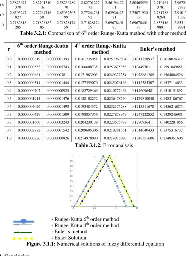
- Runge-Kutta 6th order method * - Runge-Kutta 4th order method

+ - Euler’s method

- Exact Solution

Figure 3.1.1: Numerical solutions of fuzzy differential equation

4. Conclusion

Runge-42

Kutta method proposed by us is O(h3). We have proved that the sixth order Runge-Kutta

method proposed by us gives a better solution than Euler’s method and fourth order Runge-Kutta method.

REFERENCES

1. S.Abbasbandy, J.J.Nieto and M.Alavi, Tuning of reachable set in one dim fuzzy differential inclusions, Chaos, Solutions and Fractals, 26 (2005) 1337-1341.

2. S.Abbasbandy and T.Allah Viranloo, Numerical solution of fuzzy differential

equations by Taylor’s method, Journal of Computational Methods in Applied Mathematics, 2(2) (2002) 113-124.

3. S.Abbasbandy and T.Allah Viranloo, Numerical solution of fuzzy differential

equations by Runge-Kutta method, Nonlinear Studies, 11(1) (2004) 117-129.

4. J.J.Buckley, E.Eslami and T.Feuring, Fuzzy Mathematics in Economics and

Engineering, Heidelberg, Germany, Physics-Verlag, 2002.

5. J.J.Buckley and T.Feuring, Fuzzy differential equations, Fuzzy Sets and Systems, 110 (2000) 43-54.

6. J.C.Butcher, The Numerical Analysis of Ordinary Differential Equations by

Runge-Kutta and General Linear Methods, New York, Wiley, 1987.

7. S.L.Chang and L.A.Zadeh, On fuzzy mapping and Control, IEEE Transactions on

System Man Cybernetics, 2(1) (1972) 30-34.

8. D.Dubois and H.Prade, Towards fuzzy differential calculus: Part 3, ifferentiation, Fuzzy Sets and System, 8 (1982) 225-233.

9. D.Goeken and Johnson, Runge-Kutta with higher order derivative approximations,

Applied Numerical Mathematics, 34 (2000) 207-218.

10. R.Goetschel and W.Voxman, Elementary fuzzy calculus, Fuzzy Sets and Systems, 18

(1986) 31-43.

11. O.Kaleva, Fuzzy differential equations, Fuzzy Sets and Systems, 24 (1987) 301-317.

12. O.Kaleva, The Cauchy’s problem for ordinary differential equations, Fuzzy Sets and

Systems, 35 (1990) 389-396.

13. J.D.Lambert, Numerical methods for ordinary differential systems, New York,

Wiley, 1990.

14. M.Ma, M.Friedman and M.Kandel, Numerical solution of fuzzy differential

equations, Fuzzy Sets and Systems, 105 (1999) 133-138.

15. S.Ch.Palligkinis, G. Papageorgiou, Ioannis Th. Famelis, Runge-Kutta methods

for fuzzy differential equations, in: Applied Mathematics and Computation,

2009.

16. M.L.Puri and D.A.Ralescu, Differential of fuzzy functions, Journal of Mathematical

Analysis and Applications, 91 (1983) 552-558.

17. S.Seikkala, On fuzzy initial value problem, Fuzzy Sets and System, 24 (1987)