Copyright © 2013 IJECCE, All right reserved
Texture Based Image Classification
J. Gayatri, Vani.N, Hanumantha Reddy, Siddalingesh.G
Department of Instrumentation and Technology and Computer Science, VTU UniversityR.Y.M.E.C Engineering College, Bellary
Email: [email protected], [email protected].{udbal38,siddug123}@gmail.com
Abstract - Texture classification is one of the four problem domains in the field of texture analysis. Here the approach for classification is based on the segmentation procedure that is used. The task of unsupervised texture segmentation has been the challenge of intensive research which attempts to discriminate between regions which have different textures. This paper addresses the textured image classification issue using the statistical based approach for extracting the spatial structures. Further level set method is used to analyze the feature space in order to extract homogeneous regions. This method is able to retrieve the texture regions and recover the shape from texture information in images. The approach for classification is based on moment features for segmentation. Based on the type of moments we are going to classify the images, these images are particularly from brodatz album. This work is poised on using the difference in mean and the standard duration of various features such as orientation and contrast, further using the level sets method for extracting the homogeneous regions. The statistical features are extracted using a window of suitable size around each pixel. Here we are trying to explore the possibility of using windows of different shapes and their benefits in segmenting the textures. As this method uses the difference in the first order statistical quantity, it yields the results in lesser time and using of level sets makes this method a robust one.
Keywords - Brodatz, Moments, Texels, Skewness.
I. INTRODUCTION
Texture is a feature used to partition images into regions of interest and to classify those regions and provides information in the spatial arrangement of colours or intensities in an image. It characterized by the spatial distribution of intensity levels in a neighbourhood and repeating pattern of local variations in image intensity.There are three approaches to defining exactly what texture is:
1. Structural:
Texture is a set of primitive Texel’s in some regular or repeated relationship.2. Statistical:
Texture is a quantitative measure of the arrangement of intensities in a region. This set of measurements is called a feature vector.3. Modeling:
Texture modeling techniques involve constructing models to specify textures. Statistical methods are particularly useful when the texture primitives are small, resulting in micro textures[1].When the size of the texture primitive is large, first determine the shape and properties of the basic primitive and the rules which govern the placement of these primitives, forming macro textures[2].
Texture is a repeating pattern of local variations in image intensity:
Fig.1. Example for texture image
Texture consists of texture primitives or texture elements, sometimes called Texel [5]. It can be described as fine, coarse, grained, and smooth, etc. Such features are found in the tone and structure of a texture. Tone is based on pixel intensity properties in the texel. While structure represents the spatial relationship between texels[4]. If texel are small and tonal differences between texels are large a fine texture results. If texels are large and consist of several pixels, a coarse texture results.
1.1 Texture Analysis
Two primary issues in texture analysis: 1. Texture classification
2. Texture segmentation
1.1.1. Texture classification
It is concerned with identifying a given textured region from a given set of texture classes. Each of these regions has unique texture characteristics Statistical methods are extensively used [6]. (e.g. GLCM, contrast, entropy, homogeneity
1.1.2 Texture segmentation
It is concerned with automatically determining the boundaries between various texture regions in an image [7]
1.1.1.1 Gray Level Co-occurrence
Copyright © 2013 IJECCE, All right reserved 594
International Journal of Electronics Communication and Computer Engineering Volume 4, Issue 2, ISSN (Online): 2249–071X, ISSN (Print): 2278–4209
where nijis the number of occurrences of the pixel values
(i,j) lying at distance d in the image. The co-occurrence matrix Pd has dimension n× n,where n is the number of gray levels in the image.
For example, if d=(1,1)
There are 16 pairs of pixels in the image which satisfy this spatial separation. Since there are only three gray levels, P[i,j] is a 3×3 matrix.
Algorithm:
• Count all pairs of pixels in which the first pixel has a value i, and its matching pair displaced from the first pixel by d has a value of j.
• This count is entered in the ithrow and jth column of the matrix Pd[i,j]
Normalized GLCM N[i,j], defined by:
N[i,j]= [ , ]
∑ ∑ [ , ]
This normalizes the co-occurrence values to lie between 0 and 1, and allows them to be thought of as probabilities.
1.1.2.1 Segmentation of Texture
A dictionary-like definition of texture segmentation would be the following: the partitioning of an image into regions, each of which contains a single texture distinct from its neighbors [4]. However, this definition does little to explain the inherent difficulties and practical limitations involved in this problem. To start with, we should consider the two terms ``texture'' and “segmentation'' separately [8]. Mathematically, image segmentation is well-defined [6] . An image consists of an array of pixels, and we want to give each pixel a label [8]. A region consists of a connected group of pixels that share the same label. We wish to partition an image into regions of homogeneous texture, but we cannot always agree on when two texture samples are similar to each other [8]. Furthermore, two different objects with a common boundary may have the same texture and be lumped together, which may or may not be desired [2]. Texture segmentation will invariably break up certain objects which contain multiple textures, and group together pieces of different objects into one region.
II. TYPES OF
TEXTURE
SEGMENTATION
Texture segmentation is to segment an image into regions according to the textures of the regions. One of the most fundamental choices is that between supervised texture segmentation and unsupervised texture segmentation [3]. In the supervised texture segmentation, it is assumed that all the parameters for the textures, and for the noise if it is present, are specified and the segmentation is to partition the image in terms of the textures whose distribution functions have been completely specified[9]. Unsupervised segmentation not only does the partition but also needs to estimate the involved parameters. The difference between the two can
be summed up in the a priori knowledge about the specific task that the algorithm is trying to address. If it is believed that the number of different textures is small, and that the textures are distinct from each other, then we can delineate small regions of homogeneous texture, extract feature vectors using our model, and use these vectors as ``fixed points'' in feature space[8]. Now all vectors can be labeled by assigning them the label of their closest neighbor that is a fixed point [2]. By using neural networks or other machine learning algorithms, the system can be told when it makes mistakes, and it can adjust its model accordingly.
If the number of possible textures is too large, or if no assumptions can be made about the type of textures to be presented to the system, then unsupervised methods must be used. Whereas before each feature vector could be assigned to a class as it was generated, here statistical analysis must be performed on the entire distribution of vectors [7]. The goal is to recognize clusters in the distribution and assign the same label to them all. In general, this is a much harder task to accomplish [2]. However, neither method will work properly in the absence of a function that can take two feature vectors and compute a number which represents the perceptual distance between the two windows [1]. If the parameters are homogeneous it may be possible to use the simple Euclidean metric to compute distance. However, it is almost always the case that a more complicated function must be used, one that at the very least normalizes the differences between different components [7]. And yet, some components may be more important for discrimination purposes than others, so it makes sense to weight them more highly. Often this leads to a distance function that is a heuristic based on experimentation and intuition rather than formal mathematical principles.
III. LEVEL
SETS
Level set methods provide mathematical and computational tools for tracking evolving interfaces with sharp corners and cusps, topological changes, and 3-D complications. Armed with these level set techniques, we can efficiently compute solutions to problems in geometry, fluid mechanics, and computer vision and material sciences [4]. Consider two separate circular flames, each burning outwards at a constant speed: the shape of the evolving interface is easily predicted.
Fig.2. Initial flame arising with time
Copyright © 2013 IJECCE, All right reserved
3.1. A level set representation
Rather than follow the interface itself, the level set approach instead takes the original interface and adds an extra dimension to the problem [5]. Recalling the previous interface which consisted of two expanding circular blue flames, here we introduce a co-ordinate system, using the
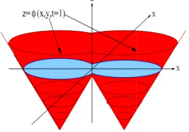
xy plane which contains the interface, and a z direction to
measure height. Suppose we invent a function z=φ(x, y, t=0),just as was done previously to take as input a point(x, y), and assigns a height z. This time, however, assign as
height z the distance from (x, y) to the interface at time
t=0.This builds a surface (shown in red) with the property
that it intersects the xy plane exactly at the interface. The red surface is called the level set function, because it accepts as input any point in the plane and hands back a height as output. The blue interface is called the zero level set, because it is the collection of all points that are at height zero.
Fig.3. The level set surface (in red) plots the distance from each point (x.y) to the interface (in blue)
Our plan is to figure out how to change the height of the surface φ (x, y, t) in time to match the evolution of the
interface [8]. The goal is to let the level set function expand, rise, fall, and do all the work: to find out where the interface is at any time, we can simply cut the surface at zero height, in other words, plot the zero contours [5].
Observe that in figure below, two expanding flames which merge into one simply means that the zero level set at a particular time becomes one curve rather than two.
Fig.4. Later in time: red level set surface has moved, yielding new blue interface
The reason it is called an "initial value formulation" is because the initial position of the interface gives initial data for a time-dependent problem i.e., the solution starts
at a given position and evolves in time. In other words, the level set approach introduced by Osher and Sethian instead takes the original curve (the red one on the left below), and builds it into a surface. That cone-shaped surface, which is shown in blue-green on the right below, has a great property; it intersects the xy plane
exactly where the curve sits. The blue-green surface on the
right below is called the level set function, because it accepts as input any point in the plane and hands back its height as output. The red front is called the zero level set, because it is the collection of all points that are at height zero.
The original front The level set function
Fig 4: Level set representation
3.1.1. Advantages of using level sets:
i) It is easy to build accurate numerical schemes to approximate the equations of motion.
ii) Relatively fine resolution can be achieved.
iii) Efficient handling of slightly tilted lines and corners. iv) The precise and easy calculation of surfacenormal’s. v) Joining of surfaces is implicitly handled by the
algorithm.
3.2. Chan and vese model:
Level set is a higher dimensional distance mapped function embedding the deformable curve as reference zero valued level set. The evolution which is due to geometrical properties of curve is further coupled with the image data to recover the object boundaries. The model proposed by Chan and Vese, does not require the boundary descriptor of the image for the stopping process.
3.2.1. Description of the chan and vese model:
In the simplest case, assume that an image I defined on Ω is composed of two regions separated by initialized model curve with homogeneous intensity values ciand co.
Given a curve C that corresponds to boundary descriptor of the image I, they introduced homogeneity – based functional
1 2 1 2 ) ( outsideC o insideCi d I C d
C I C
E
………..(3.2.1) where, ci and coare the average image intensities inside
and outside of the model propagating curve C respectively. Assuming q is the piece wise approximated model having intensity ciinside C and cooutside C, it is easy to observe
that q can be represented as
q= CiH (Φ) + Co(1-H(Φ)) ……... (3.2.2) Copyright © 2013 IJECCE, All right reserved
3.1. A level set representation
Rather than follow the interface itself, the level set approach instead takes the original interface and adds an extra dimension to the problem [5]. Recalling the previous interface which consisted of two expanding circular blue flames, here we introduce a co-ordinate system, using the
xy plane which contains the interface, and a z direction to
measure height. Suppose we invent a function z=φ(x, y, t=0),just as was done previously to take as input a point(x, y), and assigns a height z. This time, however, assign as
height z the distance from (x, y) to the interface at time
t=0.This builds a surface (shown in red) with the property
that it intersects the xy plane exactly at the interface. The red surface is called the level set function, because it accepts as input any point in the plane and hands back a height as output. The blue interface is called the zero level set, because it is the collection of all points that are at height zero.
Fig.3. The level set surface (in red) plots the distance from each point (x.y) to the interface (in blue)
Our plan is to figure out how to change the height of the surface φ (x, y, t) in time to match the evolution of the
interface [8]. The goal is to let the level set function expand, rise, fall, and do all the work: to find out where the interface is at any time, we can simply cut the surface at zero height, in other words, plot the zero contours [5].
Observe that in figure below, two expanding flames which merge into one simply means that the zero level set at a particular time becomes one curve rather than two.
Fig.4. Later in time: red level set surface has moved, yielding new blue interface
The reason it is called an "initial value formulation" is because the initial position of the interface gives initial data for a time-dependent problem i.e., the solution starts
at a given position and evolves in time. In other words, the level set approach introduced by Osher and Sethian instead takes the original curve (the red one on the left below), and builds it into a surface. That cone-shaped surface, which is shown in blue-green on the right below, has a great property; it intersects the xy plane
exactly where the curve sits. The blue-green surface on the
right below is called the level set function, because it accepts as input any point in the plane and hands back its height as output. The red front is called the zero level set, because it is the collection of all points that are at height zero.
The original front The level set function
Fig 4: Level set representation
3.1.1. Advantages of using level sets:
i) It is easy to build accurate numerical schemes to approximate the equations of motion.
ii) Relatively fine resolution can be achieved.
iii) Efficient handling of slightly tilted lines and corners. iv) The precise and easy calculation of surfacenormal’s. v) Joining of surfaces is implicitly handled by the
algorithm.
3.2. Chan and vese model:
Level set is a higher dimensional distance mapped function embedding the deformable curve as reference zero valued level set. The evolution which is due to geometrical properties of curve is further coupled with the image data to recover the object boundaries. The model proposed by Chan and Vese, does not require the boundary descriptor of the image for the stopping process.
3.2.1. Description of the chan and vese model:
In the simplest case, assume that an image I defined on Ω is composed of two regions separated by initialized model curve with homogeneous intensity values ciand co.
Given a curve C that corresponds to boundary descriptor of the image I, they introduced homogeneity – based functional
1 2 1 2 ) ( outsideC o insideCi d I C d
C I C
E
………..(3.2.1) where, ci and coare the average image intensities inside
and outside of the model propagating curve C respectively. Assuming q is the piece wise approximated model having intensity ciinside C and cooutside C, it is easy to observe
that q can be represented as
Copyright © 2013 IJECCE, All right reserved 596
International Journal of Electronics Communication and Computer Engineering Volume 4, Issue 2, ISSN (Online): 2249–071X, ISSN (Print): 2278–4209
where, the Heaviside function H (Ф) is defined as
0 , 0
0 , 1 ) (
H ……….(2.2.3)
3.2.2 Advantages of Chan and Vese model:
i) Allows arbitrary initialization of the contourii) Depending on a particular feature derived from the image, it allows for boundary detection
iii) It avoids re-initialization of intermediate contours during propagation.
The main drawback is that it is applicable only to images with finite gray level and not natural images.
IV. IMPLEMENTATION
This implementation uses either of the moment descriptors based on the texture image viz. mean, standard deviation and 3rd order moment of texture images over a predefined neighborhood. Further, the level sets method is used on the derived feature image for extracting the homogeneous regions. Level set is a higher dimensional distance mapped function embedding the deformable curve as reference zero valued level set. The curve used for segmentation is evolved using geometrical properties of the curve. The evolution is further coupled with the image data to recover the object boundaries. The model proposed by Chan and Vese, does not require the boundary descriptor of the image for the stopping process. The stopping term is based on Mumford– Shah’s piece -wise model. This model can detect contours with and without the edge descriptors. With this model the desired regions are automatically detected with the initial curve being anywhere in the image.
4.1. Moment Descriptors
Some of the definitions are defined which are useful for calculating and analyzing the results
4.1.1. Mean:
In statistics, mean has two related meanings:The arithmetic mean (and is distinguished from the geometric mean or harmonic mean).
The expected value of a random variable, which is also called the population mean.
Arithmetic mean:
The arithmetic mean is the "standard" average, often simply called the "mean".
X=1/n*∑ i…………(4.1)
4.1.2. Standard deviation:
In probability theory and statistics, standard deviation is a measure of the variability or dispersion of a population, a data set, or a probability distribution. A low standard deviation indicates that the data points tend to be very close to the same value (the mean), while high standard deviation indicates that the data are “spread out” over a large range of values.
Definition:
Let Xbe a random variable with mean value μ: E[X] = ……… (4.2)
Here the operator E denotes the average or expected value of X. Then the standard deviation of X is
= [( − )2]……….. (4.3)
4.1.3. Skewness (3rd order moment):
The third central moment is a measure of the lopsidedness of the distribution; any symmetric distribution will have a third central moment, if defined, of zero. The normalized third central moment is called the skewness, often γ. A distribution that is skewed to the left (the tail of the distribution is heavier on the left) will have a negative skewness. A distribution that is skewed to the right (the tail of the distribution is heavier on the right), will have a positive skewness.
The skewness of a random variable X is the third standardized moment, denotedγ1and defined as
= = = ( )
( [( ) ]) = ... (4.4) Whereμ3is the third moment about the meanμ,σis
the standard deviation, and E is the expectation operator. The last equality expresses skewness in terms of the ratio of the third cumulantκ3and the 1.5th power of the second
cumulantκ2. This is analogous to the definition
of kurtosis as the fourth cumulant normalized by the square of the second cumulant. The skewness is also sometimes denoted Skew[X].
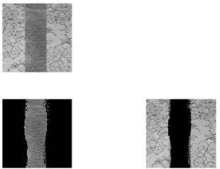
Fig.5. Top left-original image, Top right-mean of a image, Bottom left-standard deviation of a image, Bottom
right-3rd moment of a image.
V. ISSUE OF
WINDOW
SIZE AND
SHAPE
In general the window size also plays a decisive role for use of moment descriptors in segmenting texture regions. As the window size gets larger, more global features are detected. This suggests that the choice of window size could possibly be tied to the contents of the image. The images with larger texture tokens would require larger window sizes whereas finer textures would require smaller windows.
The window size may be even tied to the frequency content of image. However, the larger choice of window increases the uncertainty along the region boundaries. On the other hand if the window size is too small, it becomes difficult to capture the variations for certain textures. The execution time is less for small window sizes i.e., as the window size increases, the more time it takes for yielding a result.
5.1. Issue of Selection of Moments
Copyright © 2013 IJECCE, All right reserved homogeneous neighborhood. The moments are vital
attributes for good segmentation. The moments are calculated around each pixel within a suitable sized square window. The first moment which is the mean gives out best features when the mean of the different regions are not same. If similar intensities are distributed within a region the second moment is selected as the feature energy term. The second moment gives the spread of the distribution around the mean. For the regions with intensities that are symmetrically distributed about the mean, the third moment or skew gives the best feature energy term and is selected as the feature to embed into the level set frame work.
VI. RESULTS
& DISCUSSIONS
All results are presented using simplified motion PDE. The results are presented with combination of two texture regions derived from Brodatz’s data base.Irefis computed
using the coefficient αiequal to 1 and moment descriptors
used are to the maximum order of 3. Each image below is internally arranged as follows: Top left: original image, top right: respective moment, bottom: segmented images. The results of the segmentation algorithm show that the image moments computed over local regions provide a powerful set of features that reflect certain textural properties in images. Textures which contain higher spatial frequencies requires smaller window size. (i.e. those with lower spatial frequencies) require larger windows and those with lower spatial frequencies require larger windows.
Fig.6. Results obtained with mean (1storder moment) descriptor.
Fig.7. Results obtained with standard deviation (2ndmoment) descriptor.
Fig.8. Results obtained with skew (3rdmoment) descriptor Table 1: Window size and type of moment required for
image segmentation.
Image Window
size
Type of moment
1 3*3 mean
2 3*3 mean
3 3*3 mean
4 3*3 mean
5 3*3 Standard
deviation
6 5*5 Standard
deviation
7 21*21 skew
8 9*9 skew
9 9*9 skew
10 21*21 skew
Classification of images from brodatz album based on moments using segmentation
Table 2: The numbers in the table indicate the image numbers from the Brodatz album.
Moment 1
Moment 2
Moment 3
4 1 19
6 8 24
10 12 37
11 44 39
25 48 40
33 51 41
46 101 42
47 103 88
VII. CONCLUSION
Copyright © 2013 IJECCE, All right reserved 598
International Journal of Electronics Communication and Computer Engineering Volume 4, Issue 2, ISSN (Online): 2249–071X, ISSN (Print): 2278–4209
“corner-closure” type texture patterns show that the important aspects of the textural properties have been captured by this representation. Certain aspects of our algorithm need to be studied more carefully. First, the size of the window within which the moments are computed can be regarded as a scale parameter. This can be seen easily with the zero-order moments where the moment window size corresponds to the size of a box averaging window which is obviously a scale parameter. This window size depends on the content of the image: finer textures require a smaller window size in order to detect smaller features, whereas coarser textures require larger windows.
REFERENCES
[1] A.C. Bovik, M.Clark, and W.S.Geisler, “Multi channel texture analysis using localized spatial filters”, IEEE trans. Pattern Anal.
Mach Intell., Vol.12, No.1, pp 55–73, Jan 1990.
[2] T.F.Chan, L.A.Vese, Active contours with out edges, IEEE trans. on image process., 10, 2001, 266-276.
[3] T.Chang and C.Kuo, “Texture analysis and classification with tree structured wave let transform”, IEEE trans. image process
Vol.11, No.2, pp 429–441, Oct. 1993.
[4] Chen Sagiv,Nir A. Sochen,and Yeshoshua Y.Zeevi,”Integrated Active Contours for Texture Segmentation,” IEEE trans. image
process Vol.15, No.6, pp 1633–1646, June 2006.
[5] R.Conners and C.Harlow, “A theoretical comparison of texture
algorithms,” IEEE trans. Pattern Anal. Mach. Intell, Vol.2,
No.PAMI-3, pp.204-222, May 1980.
[6] D.Dunn and W.Higgins, “Optimal Gabor filters for texture segmentation,” IEEE trans, image process., Vol.4, No.7. pp.947 -964, July 1995.
[7] A.Laine and J.Fan, “texture classification by wave let packet signatures,” IEEE trans, pattern Anal. Mach. Intell., Vol.15,
No.11. pp.1186-1191, Nov.1993.
[8] Mumford.D and Shah.J optimal approximation by piece wise smooth function and associated variational problems. Commun.Pure Appl. Math,42, 1989, 577-685.
[9] Sandeep v. m.and Subhash Kulkarni “Efficient Hierarchical
approach for perceptual segmentation using Multi-phase Level
Sets,”
[10] Sandeep v. m.and Subhash Kulkarni “Curve Invariant Fast
Distance Mapping Technique for Level Set.
AUTHOR
’
SPROFILE
J. Gayatri
The author J.Gayatri is of native from Bellary District of Karnataka, India. She Born at Date-of-birth is 12-1-1986.This author completed M.Tech in Digital Electronics form BITM, Bellary. She is working as Assistant Professor in IT department, RYM Engineering college of Bellary from past Three years. Her area of interest includes Image processing. Email: [email protected]
Vani.N
The author VANI .N is of native from Bellary District of Karnataka, India. She Born at Date-of-birth is 16-12-1987.This author completed M.Tech in Computer Networking form AMC Engineering College. She is working as Assistant Professor of CSE department in RYMEC college of Engineering and Technology, Bellary, for the past Two years. Her area of interest includes Cloud Computing. Email: [email protected]
Hanumantha Reddy
The author Hanumantha Reddy is of native from Bellary District of Karnataka, India. Born at Date-of-birth 5-10-1988.This author completed M.Tech in Power Electronics form PDA Engineering College. He is working as Assistant Professor of IT department in RYMEC college of Engineering and Technology, Bellary, for the past one years. His area of interest includes Image processing, power electronic Drives.
Email: [email protected]