Modeling of cylindrical composite shell structures based on the Reissner’s Mixed Variational Theorem with a variable separation method

R E S E A R C H A R T I C L E

Open Access

Modeling of cylindrical composite shell

structures based on the Reissner’s Mixed

Variational Theorem with a variable

separation method

Philippe Vidal*, Olivier Polit, Laurent Gallimard and Michele D’Ottavio

*_{Correspondence:}

[email protected] LEME, UPL, Univ Paris Nanterre, 50 rue de Sèvres, 92410 Ville d’Avray, France

Abstract

This work deals with the modeling of laminated composite and sandwich shells through a variable separation approach based on a Reissner’s Variational Mixed Theorem (RMVT). Both the displacement and transverse stress fields are approximated as a sum of products of separated functions of the in-plane coordinates and the transverse coordinate. This approach yields to a non-linear problem that is solved by an iterative process, in which 2D and 1D problems are separately considered at each iteration. In the thickness direction, a fourth-order expansion in each layer is used. For the in-plane description, classical Finite Element method is used. Numerical examples involving several representative shell configurations (deep/shallow, thick/thin) are addressed to show the accuracy of the present method. It is shown that it can provide quasi-3D results less costly than classical LW computations. In particular, the estimation of the transverse stresses, which are of major importance for damage analysis, is very good.

Keywords: Composite, Shell, Separation of variables, RMVT

Introduction

Composite shells are widely used in the industrial field (aerospace, automotive, marine, medical industries...) due to their excellent mechanical properties, especially their high specific stiffness and strength. For composite design, accurate knowledge of displacements and stresses is required. One way consists in considering the three-dimensional modeli-sation. However, due to the complexity of such numerical simulations, it is desirable to take advantage of the geometric ratios and to represent the problem as a two-dimensional model by referring to shell theories. There are two ways to define the approximation of the displacement field. A “pure shell” model can be considered in which the displacement is associated with the local curvilinear vectors, and strain and stress are deduced using the differential geometry [1]. Alternatively, the shell-like solid approach [2] is widely used to formulate shell Finite Element (FE), in particular in commercial software. In this case, the displacement vector is defined in the global cartesian frame. The jacobian matrix trans-formation is used to express strain and stress with respect to the reference frame defined

©The Author(s) 2019. This article is distributed under the terms of the Creative Commons Attribution 4.0 International License (http://creativecommons.org/licenses/by/4.0/), which permits unrestricted use, distribution, and reproduction in any medium, provided you give appropriate credit to the original author(s) and the source, provide a link to the Creative Commons license, and indicate if changes were made.

on the middle surface in order to introduce the constitutive law. With respect to the “pure shell” approach, differentiation is simplified and the curvatures need to be directly cal-culated [3]. The development of efficient computational models for the analysis of shells appears thus of major interest.

According to the published research, various theories for composite shells have been implemented in the FEM framework. Most of the works mentioned in the subsequent literature overview will refer to “pure shell” models restricted to a linear analysis. Following Reddy [4], two families of models can be identified:

• The Equivalent Single Layer Models (ESLM), to which belong the Classical Shell The-ory (CST/Koiter) and First Order Shear Deformation TheThe-ory (FSDT/Nagdhi). The reader can refer to [5] for a detailed description of the assumptions on the strain field to derive different shell models. CST leads to inaccurate results for composites because both transverse shear and normal strains are neglected, see [6–8] for shallow laminated shells. FSDT is the most popular model due to the possibility to use a C0_FE, but it needs shear correction factors and the transverse normal strain is still neglected (cf. [9–12]). So, Higher-order Shear Deformation Theories (HSDT) have been devel-oped to overcome these drawbacks. Different kinematics including 7 [13,14] or 9 parameters [15] have been proposed. Reddy has derived a 5 parameter model starting from a third-order theory by considering the homogeneous top/bottom conditions for the transverse shear stresses [16]. Note also the variable kinematics approach based on the Carrera’s Unified Formulation developed in [17,18].

In the ESLM context, a simple way to improve the estimation of the mechanical quantities consists in adding one zig–zag function, called Murakami’s function, in the expression of the displacement. In this way, the slope discontinuity at the interface between two adjacent layers is introduced. It allows to describe the so-called zig–zag effect. It has been carried out in conjunction with the FSDT in [19] and [20] based on dedicated mixed formulation. It has been also used with the HSDT in [21] and [22] including 9 and 13 parameters, respectively.

• The Layer-Wise Models (LWM), in which the expansion of the mechanical quan-tities is defined over each layer independently. Some of these works are based on a linear distribution of the in-plane displacements through each layer, without tak-ing into account the transverse normal stress. The transverse displacement can be constant across the whole thickness, such as in [23,24], or in each layer separately, as in [25]. But, this type of approach fails to predict accurate transverse stresses, unless using dedicated post-processing steps [24]. Thus, higher-order approaches taking into account the transverse normal effect have been developed. The three-dimensional constitutive law is used. Second-, third- and fourth-order expansions are discussed in [4,26,27]. In this framework, Kulikov [28] has developed the sampling surfaces method, see also the previously mentioned work [18]. In all the aforemen-tioned LWM, the number of unknowns depends on the number of layers, which may thus affect the performance in terms of computational cost.

unknowns becomes independent of the number of layers. The deduced model can be derived from the CST [29], as well as from an HSDT with a third-order theory [30–33] or the sinus model [1]. The number of parameters of the resulting displacement model varies from 5 to 15. We can also cite two other approaches where only the displacement continuity [34] or the top/bottom conditions [16] are satisfied. While the above refer-ences propose models still relying on the 2D constitutive law, the papers [35,36] extend the zig–zag approach to include the transverse normal stress.

It should be noted that the mentioned works are based on the Finite Element method for linear elasticity problem in mechanics and applied to laminated composites, knowing that many other approaches (meshless, analytical, semi-analytical...) are involved in open literature. Furthermore, the fundamental subject about the shear and membrane locking of shell is not addressed here. So, this above literature deals with only some aspects of the broad research activity about composite shells. An extensive assessment of different approaches for various theories and/or finite element applications can be found in [37–45] and more recently in [46].

Nevertheless, in the framework of the failure analysis of composite structures, involving the free edge effect for instance, the prediction of the interlaminar stresses is of major interest. In particular, the difficulty is to well-describe the interlaminar continuous trans-verse stresses. Most of the ESLM fail to represent these in the most critical cases, unless using a post-processing treatment [11,24,47–49]. To overcome these drawbacks, alter-native formulations to the displacement-based approach have been developed. On the one hand, several techniques have been devised to correct the transverse shear locking pathology affecting FSDT-based plate/shell elements, most of which can be stated from hybrid-mixed approaches [50]. For composites, an assumed strain approach has been adapted in a FSDT [51] or in a LWM [52]. On the other hand, assumed partial/complete stress field over the laminate thickness independently aims at increasing the accuracy of this one. Without considering the transverse normal stress, some authors [53,54] have adopted a partial hybrid stress approach based on the HellingerReissner Variational Prin-ciple (HRVP). Using a HSDT approach for displacements, Yong [53] has developed a generalized stress assumption for the transverse shear stresses only, whereas in-plane stresses are also involved in [54]. Alternative hybrid approaches take into account the transverse normal effect. The Fraeijs de VeubekeHuWashizu multifield variational prin-ciple [55,56] and the Reissner Mixed Variational Theorem [57] are used assuming the transverse shear stresses only. Note that Sgambitterra et al. [14] have introduced a mixed-field assumptions (γ_α3andσ33) to derive a hybrid formulation enforcing the compatibility straindisplacement relations to be least-squares compatible through the shell thickness. As a complement to these hybrid methods, mixed formulations are addressed in conjunc-tion with FSDT [58] (HRVP) or including the Murakami’s zig–zag function [20] (Jing and Liao’s functional [59]). An advanced method is proposed in [60] by considering all inter-laminar stresses between two adjacent layers as primary variables and also a higher-order LW displacement.

approach comes from the works of Reissner, see [61,62]. It was first applied for multi-layered structures in [63] and then, in [64] with higher order displacement field and [65] with a Layerwise approach for both displacements and transverse stress fields. Afterwards, the approach was widely developed with a systematic approach based on the Carrrera’s Unified Formulation to provide a large panel of 2D models for composite structures based on ESL and/or LW descriptions of the unknowns [66–68]. It has been also applied for shell structures in [69–71]. Note that the reader can refer to [27] for a survey on RMVT in this framework, and to [37,72] for a further discussion.

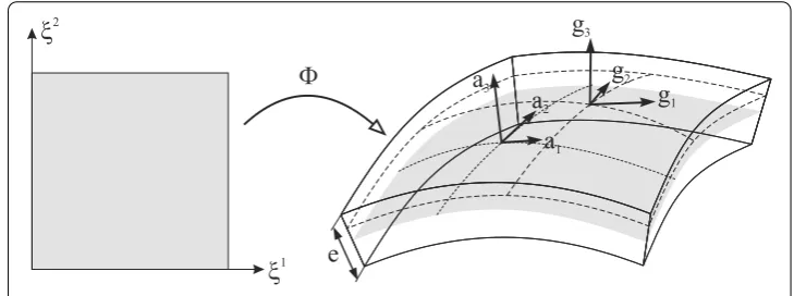
Fig. 1 The mapand the local basis vectorsaiandgifor a shell panel

Shell definitions and differential geometry

A shellCwith a middle surfaceSand a constant thicknesse, see Fig.1, is defined by [84]:

C=

M∈R3:OM( ξ,ξ3=z)= (ξ)+za3;ξ ∈;− 1 2e≤z≤

1 2e

where the middle surface can be described by a map from a parametric bidimensional domainas:

:⊂R2−→S ⊂R3

ξ =(ξ1,ξ2) −→ (ξ) (1)

In Fig.1, the map describing the shell middle surface (in grey) and the local basis vectors are presented. The basis vectors ai are defined for a point on S and the basis vectorsgiare defined for a generic point of the shell.

For a point on the shell middle surface, the covariant basis vectors defining the tangent plane to the middle surface are usually obtained as follows:

a_α = (ξ1,ξ2),α; a3= a1× a2

||a1× a2||

(2)

wherea3is the unit normal vector to the surfaceS, see Fig.1. In Eq. (2) and further on, latin indicesi, j,. . .take their values in the set{1,2,3}while greek indicesα,β,. . .take their values in the set{1,2}. The summation convention on repeated indices is used and partial derivative is denoted by (),_α. A shell is characterized by the first fundamental form a_αβ and the second oneb_αβ. Their covariant, contravariant and mixed form definitions are given by:

a_αβ = a_α.a_β aαβ = aα.aβ b_αβ = a_α,β.a3 bβα= aβ.a3,α (3)

The contravariant vectors are constructed from the covariant ones using the following equations:

aα.a_β =δα_β a3= a3; gα.gβ =δβα g3= g3 (4)

whereδα_βis the Kronecker symbol.

For a generic point of the shell, covariant basis vectors must be defined and we have

g_α= OM(ξ, z),α =(δβ_α−zbβα)aβ =μβα(z)aβ and g3= a3 (5)

introduced in Eq. (5) defines the transport from the shell middle surface to any point of the shell and is associated with the curvature variation along the thickness directionzof the shell. The inverse tensor of the mixed tensorμβ_αis denotedmβ_αand is defined as:

mβ_α =(μ−1)β_α = 1

μ{δβα+z(bβα−2Hδβα)} (6)

where we have introduced the determinant of the mixed tensor μ = det(μβ_α) = 1−2Hξ3+(ξ3)2K and the invariants of the second fundamental formH = 1₂tr(bβ_α) andK =det(bβ_α). Finally, the surface elementdSand the volume elementdCare given by:

dS=√a dξ1dξ2 dC=μdSdz (7)

where ais the determinant of the first fundamental forma_αβ. The geometry of a shell can also be defined using contravariant or mixed forms. Furthermore, covariant and con-travariant differentiation involving Christoffel symbols are not detailed here and readers can refer to the book [84].

Reference problem description

The definition of the strain field

For geometrically linear elastic analysis, the components of the strain tensorεijexpressed in the contravariant basisaiare obtained through covariant differentiation, denoted|, as follows:

ε=εij(ai⊗ aj) with

2ε_{γ λ}=mβ_λ u_γ|β−b_{γ β}u3+mαγ u_λ|α−b_λα u3 2ε_γ3=uγ|3+mαγ

u3,α+bλα uλ

ε33=u3,3

(8)

The mixed tensormβ_λcarries out the transport from any point of the shell to the shell middle surface, that is fromgitoai.

Constitutive relation

The stress tensor is obtained from the strain tensor using the constitutive equations. For this purpose, all these tensors must be referred to the covariant and contravariant basis vectors,aiandairespectively, associated with the middle surface of the shell. In case of laminated shells composed of orthotropic plies, this reference frame ensures to consis-tently take into account the different material orientations of the layers. The tensorial relation is:

σij _=Qijkl_ε

kl withσij(ai⊗ aj), Qijkl(ai⊗ aj⊗ ak⊗ al), εkl (ak⊗ al) (9)

It should be noted that the stress tensor is defined in the covariant reference frame, whereas the strain components are defined in the contravariant frame. If the frame is assumed to be orthonormal then covariant and contravariant components are equal, that is super-script and sub-script are interchangeable.

Firstly, stressesσand strainsεare split into two groups:

σT

p =[σ11(ξ, z)σ22(ξ, z)σ12(ξ, z)], σTn =[σ13(ξ, z)σ23(ξ, z)σ33(ξ, z)], εT

p =[ε11(ξ, z) ε22(ξ, z)γ12(ξ, z)], εTn = [γ13(ξ, z)γ23(ξ, z)ε33(ξ, z)]

(10)

where the subscriptsnandpdenote transverse and in-plane values, respectively. The shell can be made ofNCperfectly bonded orthotropic layers. Using the previous assumptions and the separation between transverse and in-plane components, the three dimensional constitutive law of thekth layer is given by:

⎧ ⎨ ⎩

σ(k) pH =Q

(k)

ppεpG+Qpn(k)εnG

σ(k) nH =Q

(k)

npεpG+Qnn(k)εnG

(11)

In this equation, the subscriptGindicates that the strain is issued from the geometrical relations, whileHmeans that the quantities are calculated from the Hooke’s law.Q(_ijk)are defined by

Q(k) pp = ⎡ ⎢ ⎢ ⎢ ⎣

Q(₁₁k) Q(₁₂k)Q₁₆(k)

Q(₁₂k) Q(₂₂k)Q₂₆(k)

Q(₁₆k) Q(₂₆k)Q₆₆(k)

⎤ ⎥ ⎥ ⎥

⎦ Q

(k) pn =Qnp(k)

T = ⎡ ⎢ ⎢ ⎢ ⎣

0 0Q(₁₃k)

0 0Q(₂₃k)

0 0Q(₃₆k)

⎤ ⎥ ⎥ ⎥ ⎦Q

(k) nn = ⎡ ⎢ ⎢ ⎢ ⎣

Q₅₅(k)Q(₄₅k) 0

Q₄₅(k)Q(₄₄k) 0

0 0 Q(₃₃k)

⎤ ⎥ ⎥ ⎥ ⎦ (12)

whereQ(_ijk)are the three-dimensional stiffness coefficients of the layer (k).

Finally, RMVT is associated to a mixed form of Hooke’s law, which can be written as

σpH =CppεpG+CpnσnM εnH =CnpεpG+CnnσnM

(13)

The assumed transverse stresses are denoted asσnM. The superscript(k)and the coor-dinates (ξ, z) are omitted for clarity reason.

The relations between the coefficients of the classical Hooke’s law Eq. (12) and the mixed one Eq. (13) are:

Cpp=Qpp−QpnQ−1

nnQnp; Cpn=QpnQnn−1 Cnp= −Q−1

nnQnp; Cnn=Qnn−1

(14)

The weak form of the boundary value problem

The formulation of the problem is based on the Reissner’s partially Mixed Variational Theorem [61], denoted RMVT. In this formulation, the Principle of Virtual Displacement is modified by introducing the constraint equation to enforce the compatibility of the transverse strain components. This term also depends on the assumed transverse stresses, see also [17,72]. Thus, the problem can be formulated as follows:

Findu(M)∈U(space of admissible displacements) andσnMsuch that

C

δεT

pGσpH+δεTnGσnM+δσTnM(εnG−εnH)

dC=

∂CF

δu·t d∂C

(15)

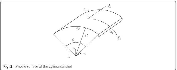
Fig. 2 Middle surface of the cylindrical shell

Application of the proper generalized decomposition to the cylindrical shell In this section, we develop the application of the PGD for shell analysis with a mixed formulation. This work is an extension of a previous study on composite cylindrical shell structures [79].

The cylindrical geometry

A cylindrical shell (see Fig.2) is described using the following map: ⎧ ⎪ ⎪ ⎪ ⎪ ⎨ ⎪ ⎪ ⎪ ⎪ ⎩

x1(ξ1,ξ2)=Rcos _ξ1

R

x2(ξ1,ξ2)=Rsin _ξ1

R

x3(ξ1,ξ2)=ξ2

(16)

Following Eq. (3), the non-zero terms for the covariant and mixed forms are:

a11=a22=1 b11=b11= − 1

R μ

1 1=1+

z

R m

1 1=

1+ z

R ₋1

(17)

andμ=1+ z R.

The displacement and transverse stress field

Let us denote ui(ξ1,ξ2,ξ3 = z) andσi3(ξ1,ξ2,ξ3 = z) the curvilinear components of the displacement field and the transverse stresses respectively, associated with the con-travariant basis vectorsai. Letandzbe the bidimensional domain associated with the mid-surface of the shell [see Eq. (1)], and the unidimensional domain associated with the normal fiber, respectively. The displacement and transverse stress fields are constructed as the sum ofNproducts of functions of in-plane coordinates and transverse coordinate (N ∈Nis the order of the representation) according to

u=

⎡ ⎢ ⎢ ⎣

u1(ξ,ξ3=z) u2(ξ,ξ3=z)

u3(ξ,ξ3=z) ⎤ ⎥ ⎥ ⎦= N

i=1 ⎡ ⎢ ⎢ ⎢ ⎣

f₁i(z)vi₁(ξ)

f₂i(z)vi₂(ξ)

f₂i(z)f₃i(z)vi₃(ξ) ⎤ ⎥ ⎥ ⎥ ⎦= N

i=1 ⎡ ⎢ ⎢ ⎢ ⎣

f₁i(z)

f₂i(z)

f₃i(z) ⎤ ⎥ ⎥ ⎥ ⎦◦ ⎡ ⎢ ⎢ ⎢ ⎣

vi₁(ξ)

vi₂(ξ)

vi₃(ξ) ⎤ ⎥ ⎥ ⎥

⎦ (18)

σnM = ⎡ ⎢ ⎢ ⎢ ⎣

σ13(ξ,ξ3=z)

σ23(ξ,ξ3=z)

σ33(ξ,ξ3=z) ⎤ ⎥ ⎥ ⎥ ⎦= N

i=1 ⎡ ⎢ ⎢ ⎢ ⎣

f_σi₁(z)τ₁i(ξ)

f_σi₂(z)τ₂i(ξ)

f_σi₃(z)τ₃i(ξ) ⎤ ⎥ ⎥ ⎥ ⎦= N

i=1 ⎡ ⎢ ⎢ ⎢ ⎣

f_σi₁(z)

f_σi₂(z)

f_σi₃(z) ⎤ ⎥ ⎥ ⎥ ⎦◦ ⎡ ⎢ ⎢ ⎢ ⎣ τi 1(ξ)

τi 2(ξ)

τi 3(ξ)

⎤ ⎥ ⎥ ⎥

where (fi

1, f2i, f3i), (fσi1, f

i

σ2, f

i

σ3) are defined inzand (v

i

1, v2i, vi3), (τ1i,τ2i,τ3i) are defined in. The “◦” operator is Hadamard’s element-wise product.

In this paper, a classical eight-node FE approximation is used inand a LW description is chosen inzas it is particulary suitable for the modeling of composite structures.

The strain field for the cylindrical composite structure

The strain field in Eq. (8) is free of any approximated shell kinematics. These strain components are simplified using Eq. (17) and we recover the following relations:

ε11 = 1 μ

u1,1+

1 R u3

ε22 =u2,2

ε33 =u3,3

γ23=u2,3+u3,2

γ13=u1,3+ 1 μ

u3,1−

1 Ru1

γ12=u1,2+ 1 μ u2,1

(20)

where covariant derivative becomes classical derivative for the case of a cylindrical shell. Equation (18) must be introduced at this level in order to obtain the compatible strain expansion along the normal coordinatezof the shell. So, we obtain:

εpG(u)= N

j=1 ⎡ ⎢ ⎢ ⎢ ⎢ ⎢ ⎢ ⎢ ⎣

μ−1

f₁jvj_1,1+ 1 Rf j 3v j 3

f₂j v₂j_,2

f₁jv₁j_,2+μ−1f₂jv₂j_,1 ⎤ ⎥ ⎥ ⎥ ⎥ ⎥ ⎥ ⎥ ⎦ (21)

εnG(u)= N

j=1 ⎡ ⎢ ⎢ ⎢ ⎢ ⎢ ⎢ ⎢ ⎣

(f₁j)vj₁+μ−1

f₃jvj_3,1− 1 Rf j 1v j 1

(f₂j)vj₂+f₃jvj_3,2

(f₃j)vj₃

⎤ ⎥ ⎥ ⎥ ⎥ ⎥ ⎥ ⎥ ⎦ (22)

where the prime stands for the derivative with respect toz(f_i = dfi

dz), (),α indicates the partial derivative with respect toξα(α=1,2).

The problem to be solved

The resolution of Eq. (15) is based on a greedy algorithm. If we assume that the firstm functions have been already computed, the trial function for the iterationm+1 is written as

um+1_=um₊ ⎡ ⎢ ⎣

f1v1 f2v2 f3v3

⎤ ⎥

⎦=um_{+f ◦v (23)}

σm+1

nM =σmnM+ ⎡ ⎢ ⎣

f_σ1τ1 f_σ2τ2 f_σ3τ3

⎤ ⎥

⎦=σm

where (v1, v2, v3), (τ1,τ2,τ3), (f1, f2, f3) and (fσ1, fσ2, fσ3) are the functions to be computed

andum,σm_nMare the associated known sets at iterationmdefined by

um₌ m

i=1 ⎡ ⎢ ⎣

f₁iv₁i f₂iv₂i f₃iv₃i

⎤ ⎥

⎦ σm

nM = m

i=1 ⎡ ⎢ ⎣

f_σi₁τ₁i f_σi₂τ₂i fi

σ3τ

i 3

⎤ ⎥

⎦ (25)

The test functions are

δ ⎡ ⎢ ⎣

f1v1 f2v2 f3v3

⎤ ⎥ ⎦= ⎡ ⎢ ⎣

δf1v1+f1δv1

δf2v2+f2δv2

δf3v3+f3δv3 ⎤ ⎥

⎦=δf ◦v+δv◦f (26)

δ ⎡ ⎢ ⎣

f_σ1τ1 f_σ2τ2 f_σ3τ3

⎤ ⎥ ⎦= ⎡ ⎢ ⎣

δf_σ1τ1+fσ1δτ1

δf_σ2τ2+fσ2δτ2

δf_σ3τ3+fσ3δτ3

⎤ ⎥

⎦=δf_σ ◦τ+δτ◦f_σ (27)

with v= ⎡ ⎢ ⎣ v1 v2 v3 ⎤ ⎥

⎦f =

⎡ ⎢ ⎣ f1 f2 f3 ⎤ ⎥

⎦τ=

⎡ ⎢ ⎣ τ1 τ2 τ3 ⎤ ⎥

⎦f_σ =

⎡ ⎢ ⎣

f_σ1 f_σ2 f_σ3

⎤ ⎥

⎦ (28)

The test functions defined by Eqs. (26,27), the trial functions defined by Eqs. (23,24), and the mixed constitutive relation Eq. (13) are introduced into the weak form Eq. (15) to obtain the two following equations:

S

z

εpG(f ◦δv)TCppεpG(f ◦v)+Cpn(f_σ◦τ)+εnG(f ◦δv)T(f_σ◦τ)

+(f_σ◦δτ)T(εnG(f ◦v)−(CnpεpG(f ◦v)+Cnn(f_σ◦τ)))

μdz dS

=

SF

(f ◦δv)Ttμ

z=zF dS−

S

z

εpG(f ◦δv)TCppεpG(um)+CpnσmnM

+εnG(f ◦δv)TσmnM+(fσ◦δτ)T(εnG(um)−(CnpεpG(um)+CnnσmnM))

μdz dS

(29) z S

εpG(v◦δf)T

CppεpG(v◦f)+Cpn(τ◦f_σ)

+εnG(v◦δf)T(τ◦f_σ)

+(τ◦δf_σ)T_(ε

nG(v◦f)−(CnpεpG(v◦f)+Cnn(τ◦f_σ)))

dSμdz

=

SF

(v◦δf)Tt μdS

z=zF − z S

εpG(v◦δf)T

CppεpG(um)+CpnσmnM

+εnG(v◦δf)Tσm_nM+(τ◦δf_σ)T(εnG(um)−(CnpεpG(um)+Cnnσm_nM))

dSμdz

(30)

For the present work,∂CFis considered as the partial top or bottom surface of the shell, that isz=zF withzF = ±e/2.

From Eqs. (29) and (30), a coupled non-linear problem is derived whose solution is seeked by means of a fixed point method for simplicity reason. An initial function f(0)_,f(0)

σ is set, and at each step, the algorithm computes two new pairs (v(k+1),f(k+1)),

(τ(k+1)_,f(k+1)

σ ) such that

• v(k+1),τ(k+1)satisfy Eq. (29) forf,f_σ set tof(k)andf(_σk) • f(k+1),f(_σk+1)satisfy Eq. (30) forv,τset tov(k+1),τ(k+1)

Finite element discretization

To build the shell finite element approximation, a discrete representation of the functions (v,τ,f,f_σ) must be introduced. In this work, a classical finite element approximation in andzis used. The elementary vector of degrees of freedom (dof) associated with one elementeof the mesh inis denotedqveτ, while the elementary dof vector associated with one elementz e of the mesh inz is denotedqffσe . The displacement, strain and transverse stress fields are determined from the values ofqv_eτandqffσe by

ve=Nξqveτ,Eev=Bξqveτ,τe=Nσ ξqveτ fe=Nzqffσe , Ee_f =Bzqffσe ,f_σe=Nσzqffσe

(31)

where

Ee vT =

v1v1,1v1,2v2v2,1v2,2v3v3,1v3,2

and

Ee fT =

f1f

1f2f

2f3f

3

The matricesN_ξ,B_ξ,Nz,Bz,Nσ ξ,Nσzcontain the interpolation functions, their deriva-tives and the jacobian components, respectively.

Finite element problem to be solved on

For the sake of simplicity, the functionsf(k),f(_σk)which are assumed to be known, will be denoted ˜f, ˜f_σ, respectively, and the functionsv(k+1),τ(k+1)to be computed will be denotedvandτ, respectively. The strains and the assumed transverse stresses in Eq. (29) are defined as

εpG(˜f ◦v)=pz(˜f)Ev

εnG(˜f ◦v)=n_z(˜f)Ev

σnM(˜fσ◦τ)=σ_zn(˜f_σ)τ

(32)

with

p_z(˜f)= ⎡ ⎢ ⎣

0 f˜1/μ 0 0 0 0 f˜3/(μR) 0 0

0 0 0 0 0 ˜f2 0 0 0

0 0 ˜f1 0 ˜f2/μ 0 0 0 0

⎤ ⎥

⎦ (33)

n z(˜f)=

⎡ ⎢ ⎣ ˜

f₁−˜f1/(μR) 0 0 0 0 0 0 ˜f3/μ 0

0 0 0 f˜₂ 0 0 0 0 ˜f3

0 0 0 0 0 0 f˜₃ 0 0

⎤ ⎥

⎦ (34)

σn z (˜fσ)=

⎡ ⎢ ⎣ ˜

f_σ1 0 0 0 ˜f_σ2 0 0 0 f˜_σ3

⎤ ⎥

⎦ (35)

The variational problem defined onfrom Eq. (29) is

δEvTkvz(˜f)Ev+δEvTkvzσ(˜f ,f˜σ)τ+δτTkσzv(˜f ,f˜σ)Ev+δτTkσ σz (˜fσ)τ

_√

ad =δvT_t

z(˜f)√ad−

δEvTσz(˜f ,um,σmnM)+δτTεz(˜fσ,um,σmnM)

_√

with

kv z(˜f)=

z

p_z(˜f)TCppp_z(˜f)μdz

kvσ

z (˜f ,f˜σ)=

z

n_z(˜f)Tσ_zn(˜f_σ)+p_z(˜f)TCpnσ_zn(˜f_σ)

μdz

kσv z (˜f ,f˜σ)=

z

σn

z (˜fσ)Tn_z(˜f)−_zσn(˜f_σ)TCnpp_z(˜f)μdz

kσ σz (˜fσ)= −

z

σn

z (˜fσ)TCnnzσn(˜fσ)μdz

(37)

tz(˜f)= f˜◦tμ z=zF

σz(˜f ,um,σmnM)=

z

pz(˜f)TCppεpG(um)+n_z(˜f)TσmnM+zp(˜f)TCpnσmnM

μdz

εz(˜f_σ,um,σm_nM)=

z

σn

z (˜fσ)TεnG(um)−CnpεpG(um)−CnnσmnM μdz

(38)

Note that the units ofCnn,Cnp,CpnandCppare different.

The introduction of the finite element approximation Eq. (31) in the variational Eq. (36) leads to the linear system

Kz(˜f ,f˜_σ)qvσ =Rv(˜f ,f˜_σ,um,σm_nM) (39)

where

• qvσ is the vector of the nodal displacements / transverse stresses associated with the finite element mesh in,

• Kz(˜f ,f˜_σ) is the stiffness matrix obtained by summing the elements’ stiffness

matrices Ke_z(˜f ,f˜_σ) =

e

BT

ξkvz(˜f)Bξ + BTξkvzσ(˜f ,f˜σ)Nσ ξ + NTσ ξkzσv(˜f ,f˜σ)Bξ +

NT

σ ξkσ σz (˜fσ)Nσ ξ

_√

ade

• Rv(˜f ,f˜_σ,um,σm_nM) is the equilibrium residual obtained by summing the elements’

residual load vectors Re_v(˜f ,f˜_σ,um,σm_nM) =

e

NT

ξtz(˜f)− BT_ξσz(˜f ,um,σmnM)−

NT

σ ξεz(˜fσ,um,σm_nM)

_√

ade.

Finite element problem to be solved onz

For the sake of simplicity, the functionsv(k+1),τ(k+1)which are assumed to be known, will be denoted ˜v, ˜τand the functionsf(k+1),f(_σk+1)to be computed will be denotedf,f_σ. The strain in Eq. (30) is defined as

εpG(˜v◦f)=p_ξ(˜v)E_f εnG(˜v◦f)=n_ξ(˜v)Ef σnM(˜τ◦fσ)=σ_ξn(˜τ)fσ

(40)

with

p_ξ(˜v)= ⎡ ⎢ ⎣ ˜

v1,1/μ0 0 0 ˜v3/(μR) 0 0 0 ˜v2,2 0 0 0 ˜

v1,2 0 ˜v2,1/μ0 0 0 ⎤ ⎥

n_ξ(˜v)= ⎡ ⎢ ⎣

−v˜1/(μR) ˜v10 0 ˜v3,1/μ 0 0 0 0 ˜v2 v˜3,2 0

0 0 0 0 0 v˜3

⎤ ⎥

⎦ (42)

σn

ξ (˜τ)= ⎡ ⎢ ⎣ ˜ τ1 0 0

0 ˜τ2 0 0 0 ˜τ3

⎤ ⎥

⎦ (43)

The variational problem defined on zfrom Eq. (30) is

z

δEfTkfξ(˜v)Ef +δEfTkffσξ (˜v,τ˜)fσ+δfTσkfσξf(˜v,τ˜)Ef +δfTσkfσfσξ (˜τ)fσ

μdz

= δfT_t

ξ(˜v)μ z=zF

−

z

δEfTσξ(˜v,um,σm_nM)+δfT_σε_ξ(˜τ,um,σm_nM)

μdz (44)

with

kf

ξ(˜v)=

p

ξ(˜v)TCpppξ(˜v)

√ ad

kffσ

ξ (˜v,τ˜)=

n

ξ(˜v)Tσξn(˜τ)+pξ(˜v)TCpnσξn(˜τ)

_√

ad

kfσf

ξ (˜v,τ˜)=

σn

ξ (˜τ)Tnξ(˜v)−ξσn(˜τ)TCnppξ(˜v)

_√

ad

kfσfσ

ξ (˜τ)= −

σn

ξ (˜τ)TCnnσξn(˜τ)

√ ad

(45)

and

tξ(˜v)=

v˜◦t √

ad

σξ(˜v,um,σm_nM)=

p_ξ(˜v)TCppεpG(um)+nxy(˜v)TσmnM+ξp(˜v)TCpnσmnM _√

ad

εξ(˜τ,um,σm_nM)=

σn_ξ (˜τ)TεnG(um)−CnpεpG(um)−CnnσmnM √

ad

(46)

The introduction of the finite element discretization Eq. (31) in the variational Eq. (44) leads to the linear system

Kξ(˜v,τ˜)qffσ =Rf(˜v,τ˜,um,σm_nM) (47) where

• qffσ _{is the vector of degree of freedom associated with the F.E. approximations inz,} • K_ξ(˜v,τ˜) is obtained by summing the elements’ stiffness matrices:

Ke

ξ(˜v,τ˜)=

ze BT zk f

ξ(˜v)Bz+BTzk ffσ

ξ (˜v,τ˜)Nσz

+NT

σzk fσf

ξ (˜v,τ˜)Bz+NT_σzk fσfσ

ξ (˜τ)Nσz

μdze (48)

• Rf(˜v,τ˜,um,σm_nM) = RF_f(˜v)−RCoup_f (˜v,τ˜,um,σm_nM) is a equilibrium residual with RF

f(˜v)= NTztξ(˜v)μz=zF andR

Coup

f (˜v,τ˜,um,σmnM) is obtained by the summation of the elements’ residual vectors given by

ze

BT

zσξ(˜v,um,σmnM)+NTσzεξ(˜τ,um,σmnM)

μdze (49)

Numerical results

of the shell is approximated by this classical FE in the parametric space. The geometrical transformation is based on an explicit map. A Gaussian numerical integration with 3× 3 points is used to calculate the elementary matrices.

Several static tests are presented with the aim of validating our approach and evaluating its efficiency. First, a convergence study is carried out to determine the suitable mesh for the further analysis. Then, the influence of the approximation on the factor 1/μis addressed [1,85]. Three orders of expansion are considered. The influence of the numer-ical layers is also studied to illustrate the possibility to refine the transverse description of the displacements and the stresses. The present approach is assessed for deep/shallow and thick/thin cross-ply/angle-ply/sandwich shells to show the wide range of validity.

Unless otherwise mentioned, the numerical assessments are based on the test case pro-posed by Ren [81]. It concerns a semi-infinite simply-supported cylindrical shell submitted to a sinusoidal pressure, as detailed below:

Geometry: Composite cross-ply cylindrical shell,R = 10,φ ∈ {π/8,π/3,π/2}, with the following stacking sequences [0◦], [0◦/90◦], [0◦/90◦/0◦]. All layers have the same thickness.S= R

e ∈ {2,4,10,40,100}. The panel is supposed infinite along thex2=ξ 2

direction (b_C =8a_C) (Cf. Fig.2).

Boundary conditions: Simply-supported shell along its straight edges (transverse and tangential displacements are fixed on the (ξ1,ξ2) mesh), sinusoidal pressure along

the curvature:q(ξ1)=q0sinπξ 1

Rφ

Material properties: EL =25 GPa, ET =1 GPa, GLT =0.2 GPa, GTT =0.5 GPa, νLT =νTT =0.25.

whereLrefers to

the fiber direction,T refers to the transverse direction.

Mesh: Only a quarter of the structure is meshed. The mesh is constituted ofNx ×Ny elements in theξ1andξ2directions respectively. A space ratio is considered in these two directions (ratio between the size of the larger and the smaller element). Numerical layers:Nzis the total number of numerical layers.

Number of dofs:Ndofxy = 6(3NxNy+2(Nx +Ny)+1) andNdofz = 24×αNC+6 are the number of dofs of the two problems associated withv_jiandf_jirespectively.α is the number of numerical layers per physical layer. So the total number of dofs is Ndofxy+Ndofz.

Results: The results are made nondimensional using:

¯

u=u1(0, bC/2, z)_eqET 0S3

, w¯ =u3(aC/2, bC/2, z)100ET_eq 0S4

¯

σαα = σαα(aC/2, bC/2, z)

q0S2 ,

¯

σ13= σ13

(0, b_C/2, z) q0S

, σ¯33= σ33

(a_C/2, b_C/2, z) q0

Reference values: The 2D exact elasticity results are obtained as in [81].

Few iterations are required to reach the convergence of the fixed point algorithm (cf. Section ). Moreover, for this test case, only one couple is needed to obtain the solution.

Table 1 Convergence study—one layer[0◦]—S = 40—φ=π/3—Nz =NC—meshNx×10

with space ratio (50)

Nx u(0,e/2)¯ w(L,0)¯ σ¯11(-e/2) σ¯13(0) σ¯33max

4 VS-LM4 9.3287 0.0779 −0.8406 0.3181 −8.7001

Error 0.51% 0.02% 8.79% 44.08% 22.50%

8 VS-LM4 9.3744 0.0780 −0.7908 0.5061 −7.5489

Error 0.02% 0.10% 2.35% 11.02% 6.29%

14 VS-LM4 9.3769 0.0780 −0.7786 0.5484 −7.2645

Error 0.00% 0.04% 0.77% 3.60% 2.29%

20 VS-LM4 9.3775 0.0780 −0.7756 0.5590 −7.1931

Error 0.01% 0.03% 0.38% 1.73% 1.28%

26 VS-LM4 9.3775 0.0780 −0.7744 0.5633 −7.1654

Error 0.01% 0.02% 0.22% 0.97% 0.89%

32 VS-LM4 9.3775 0.0780 −0.7738 0.5651 −7.1503

Error 0.01% 0.02% 0.14% 0.67% 0.68%

Navier 9.3778 0.0780 −0.7727 0.5688 −7.1074

Exact 9.3765 0.0780 −0.7727 0.5688 −7.1021

Fig. 3 Mesh 26_×10 with a space ratio 50 for one quarter of the shell panel—_φ=π/3–R=10

LM4: It refers to the systematic work of Carrera and his “Carrera’s Unified Formulation” (CUF), see [37,72,86]. A LayerWise model based on a RMVT approach where each component is expanded until the fourth-order, is given. 24NC+6 unknown functions per node are used in this kinematic.

VS-LD4: It refers to the work on the proper generalized decomposition with a spatial separation between (x, y) andz. A fourth-order expansion is used for the 1D problem associated to the z-direction. The formulation is based on a displacement approach (see [79]).

Convergence study

Table 2 Influence of the order-approximation of1/μwith respect toS—one layer[0◦]—φ =π/3—mesh 26×10—Nz=NC

S Expansion Model u(0, e/2¯ ) w(L,0)¯ σ¯11(-e/2) σ¯13(0) σ¯33max

2 Zero-order VS-LM4 3.9747 0.7982 −1.4093 0.4688 0.8883

Error 16.67% 19.83% 42.59% 15.76% 11.17%

2 One-order VS-LM4 4.9928 1.0179 −2.2682 0.5908 0.9324

Error 4.68% 2.24% 7.59% 6.16% 6.76%

2 Two-order VS-LM4 4.7940 0.9769 −2.1818 0.5776 0.8967

Error 0.51% 1.88% 11.12% 3.78% 10.33%

Exact 4.7696 0.9956 −2.4546 0.5565 1.0000

4 Zero-order VS-LM4 2.3665 0.2792 −1.0406 0.5287 0.9225

error 10.39% 10.50% 21.81% 7.87% 7.75%

4 One-order VS-LM4 2.6745 0.3153 −1.3452 0.5958 0.9163

error 1.28% 1.08% 1.08% 3.82% 8.37%

4 Two-order VS-LM4 2.6386 0.3112 −1.3261 0.5909 0.9062

Error 0.09% 0.25% 0.36% 2.97% 9.38%

Exact 2.6408 0.3120 −1.3309 0.5739 1.0000

10 Zero-order VS-LM4 2.5623 0.1094 −0.8071 0.5558 −1.3651

Error 4.54% 4.55% 9.30% 4.13% 9.35%

10 One-order VS-LM4 2.6932 0.1150 −0.8937 0.5838 −1.4207

Error 0.33% 0.33% 0.44% 0.69% 5.66%

10 Two-order VS-LM4 2.6846 0.1146 −0.8908 0.5829 −1.4165

Error 0.01% 0.01% 0.11% 0.55% 5.94%

Exact 2.6843 0.1146 −0.8898 0.5798 −1.5059

40 Zero-order VS-LM4 9.2631 0.0770 −0.7553 0.5564 −7.0856

Error 1.21% 1.20% 2.25% 2.19% 0.23%

40 One-order VS-LM4 9.3800 0.0780 −0.7746 0.5629 −7.1657

Error 0.04% 0.04% 0.25% 1.05% 0.89%

40 Two-order VS-LM4 9.3775 0.0780 −0.7744 0.5633 −7.1654

Error 0.01% 0.02% 0.22% 0.97% 0.89%

Exact 9.3765 0.0780 −0.7727 0.5688 −7.1021

Influence of the expansion order for the factor 1/μ

In this section, the influence of the approximation on the factor 1/μ = 1/(1+z/R) is addressed for very thick to thin homogeneous shells and for deep or shallow shells, respectively. For this purpose, the results involving the zero, one and two-order expansions are compared in Tables2and3. The zero-order approximation (thin shell hypothesis or Love’s hypothesis) seems to be suitable only for the thin structure withS≥40. ForS≤10, the order of the development of 1/μshould be increased to improve significantly the accuracy of the solution, including both the displacements and the stresses. Nevertheless, the use of the second-order expansion has a significant influence only for the thick shell.

Considering different opening angles of the structure in Table 3, it can be inferred from these results that the use of the two-order expansion allows us again to decrease significantly the error rate for both displacements and stresses. Nevertheless, the influence on the transverse normal stress does not appear for the shallow shells (φ ≤π/3).

Table 3 Influence of the order-approximation of1/μwith respect toφ—one layer[0◦]—S

=4—mesh 26×10—Nz =NC

φ Expansion Model u(0,e/2)¯ max w(L,0)¯ σ¯11(-e/2) σ¯13(0) σ¯33max

φ=π/8 Zero-order VS-LM4 0.1758 0.0206 −0.1721 0.1465 0.9699

Error 20.37% 14.13% 35.61% 8.30% 3.01%

One-order VS-LM4 0.1943 0.0237 −0.2138 0.1676 0.9782

Error 11.98% 1.10% 20.01% 4.94% 2.18%

Two-order VS-LM4 0.1925 0.0235 −0.2117 0.1670 0.9698

Error 12.79% 1.97% 20.78% 4.57% 3.02%

Exact 0.2207(-e/2) 0.0240 −0.2673 0.1597 1.0000

φ=π/3 Zero-order VS-LM4 2.3665 0.2792 −1.0406 0.5287 0.9225

Error 10.39% 10.50% 21.81% 7.87% 7.75%

One-order VS-LM4 2.6745 0.3153 −1.3452 0.5958 0.9163

Error 1.28% 1.08% 1.08% 3.82% 8.37%

Two-order VS-LM4 2.6386 0.3112 −1.3261 0.5909 0.9062

Error 0.09% 0.25% 0.36% 2.97% 9.38%

Exact 2.6408 0.3120 −1.3309 0.5739 1.0000

φ=π/2 Zero-order VS-LM4 19.7700 1.2434 −2.4271 0.9709 −1.4613

Error 9.90% 9.85% 21.19% 8.83% 15.41%

One-order VS-LM4 22.3131 1.4019 −3.1382 1.0922 −1.6628

Error 1.69% 1.63% 1.89% 2.57% 3.75%

Two-order VS-LM4 21.9662 1.3801 −3.0886 1.0822 −1.6379

Error 0.10% 0.06% 0.28% 1.62% 5.19%

Exact 21.9433 1.3793 −3.0799 1.0649 −1.7275

φ=5π/6 Zero-order VS-LM4 1268.7500 39.7516 −15.1031 4.0278 −13.0670

Error 9.01% 8.99% 20.62% 10.01% 10.39%

One-order VS-LM4 1436.1875 44.9875 −19.6075 4.5312 −14.8620

Error 3.00% 3.00% 3.05% 1.24% 1.92%

Two-order VS-LM4 1409.4375 44.1469 −19.2512 4.4970 −14.5900

Error 1.08% 1.08% 1.18% 0.48% 0.05%

Exact 1394.3688 43.6759 −19.0264 4.4756 −14.5826

the displacementuand the normal stressσ11are still high. Thus, a residual error remains. This problem is investigated in the following section.

Influence of the number of numerical layers

The influence of the number of numerical layers is studied for the homogeneous case. In Tables4and5, four numerical layers per physical layer are considered for moderately thick to very thick cases and shallow shells, respectively. These configurations are the most representative ones. First, it can be observed that the accuracy of results with different opening angles (Table5) are improved when compared with Table3, regardless of the degree of approximation. In particular, the effect on the stresses is more pronounced. Then, the use of the second order expansion of 1/μdrives to a very good agreement with the reference solution (Tables4,5). The maximum error rate is 1%, even for the very thick case. Finally, a refinement in the z-direction in conjunction with a high-order expansion of 1/μis required to obtain accurate results for the shallow shells (φ ≤ π/3) or for the moderately to very thick cases (S ≤10).

Table 4 One layer[0◦]—φ=π/3—mesh 26×10—Nz=4×NC—two-order expansion of

1/μ

S Model u(0,e/2)¯ w(L,0)¯ σ¯11(-e/2) σ¯13(0) σ¯33max

2 VS-LM4 4.7645 0.9938 −2.4609 0.5560 1.0111

Error 0.11% 0.18% 0.25% 0.09% 1.11%

Exact 4.7696 0.9956 −2.4546 0.5565 1.

4 VS-LM4 2.6411 0.3119 −1.3329 0.5720 1.0110

Error 0.01% 0.02% 0.16% 0.32% 1.10%

Exact 2.6408 0.3120 −1.3309 0.5739 1.

10 VS-LM4 2.6847 0.1147 −0.8907 0.5784 −1.5176

Error 0.02% 0.02% 0.09% 0.24% 0.77%

Exact 2.6843 0.1146 −0.8898 0.5798 −1.5059

Table 5 Influence of the order-approximation of1/μ—one layer[0◦]-S=4—mesh 26× 10—numerical layersNz=4×NC

φ Expansion Model u(0,e/2)¯ max w(L,0)¯ σ¯11(-e/2) σ¯13(0) σ¯33max

φ=π/8 Zero-order VS-LM4 −0.0085 0.0211 −0.2094 0.1415 1.0027

Error 9.30% 11.86% 21.63% 11.44% 0.27%

One-order VS-LM4 −0.0096 0.0243 −0.2694 0.1621 1.0103

Error 2.59% 1.30% 0.82% 1.48% 1.03%

Two-order VS-LM4 −0.0095 0.0241 −0.2670 0.1616 1.0023

Error 1.72% 0.46% 0.09% 1.14% 0.23%

Exact −0.0094 0.0240 −0.2673 0.1597 1.0000

φ=π/3 Zero-order VS-LM4 2.3664 0.2797 −1.0442 0.5119 1.0101

Error 10.39% 10.32% 21.54% 10.80% 1.01%

One-order VS-LM4 2.6764 0.3160 −1.3518 0.5766 1.0221

Error 1.35% 1.30% 1.57% 0.49% 2.21%

Two-order VS-LM4 2.6411 0.3119 −1.3329 0.5720 1.0110

Error 0.01% 0.02% 0.16% 0.32% 1.10%

Exact 2.6408 0.3120 −1.3309 0.5739 1.0000

expected, it can be seen that the number of numerical layers increases with the thickness of the structure. Even considering a structure with only one physical layer, the refinement of the description of mechanical quantities is required as their distributions through the thickness could be very complex for a shell structure. For illustration, the distributions of the displacement ¯uand the stresses ¯σ11, ¯σ13through the thickness are provided in Fig.4. An oscillating behavior occurs for the displacement and the in-plane stress, which is quite different than the plate case. Moreover, an asymmetrical distribution can be observed. The maximum value of the transverse shear stress is obtained near the top of the homogeneous shell.

For the present approach, it should be also noted that the additional computational cost inducing by the z-refinement is negligible as only the number of dofs of the 1D problem increases (Ndofz = 24×αNC+6, see Table6). The size of the 2D problem remains unchanged. This is a main difference with respect to a LW approach where the total number of unknowns would beNdofxy×Ndofz=Ndofxy×(24×αNC+6).

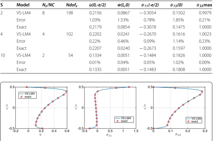
Table 6 One layer[0◦]—φ=π/8—mesh 26×10—two-order expansion of1/μ

S Model Nz/NC Ndofz u(0,-e/2)¯ w(L,0)¯ σ¯11(-e/2) σ¯13(0) σ¯33max

2 VS-LM4 8 198 0.2156 0.0867 −0.3054 0.1502 0.9979

Error 1.03% 1.53% 0.78% 1.85% 0.21%

Exact 0.2179 0.0854 −0.3078 0.1475 1.0000

4 VS-LM4 4 102 0.2202 0.0241 −0.2670 0.1616 1.0023

Error 0.22% 0.46% 0.09% 1.14% 0.23%

Exact 0.2207 0.0240 −0.2673 0.1597 1.0000

10 VS-LM4 2 54 0.1334 0.0051 −0.1484 0.1826 1.0000

Error 0.01% 0.04% 0.05% 1.02% 0.00%

Exact 0.1335 0.0051 −0.1483 0.1808 1.0000

Fig. 4 Distribution of ¯u(left), ¯_σ11(middle) and ¯_σ13(right) along the thickness—S = 2–1 layer—_φ=π/8

Fig. 5 Distribution of ¯σ13(left), ¯σ33(right) along the thickness—S = 4–3 layers—φ=π/8,π/2,5π/6

Bending analysis of laminated shells under a sinusoidal pressure

Cross-ply test case

Firstly, a thick three-layer [0◦/90◦/0◦] shell is considered, referring to the test case pro-posed by Ren [81] described in the preliminaries of the present section. Only distributions of the transverse normal and shear stresses through the thickness are provided for deep and shallow shells (see Fig.5), as those are the most difficult to obtain. Only 1 couple is built and only one element per layer is used for the problem in z. It is inferred from this figure that the present model gives excellent results when compared to the exact solution. It can be noticed that the top/bottom surface conditions are fulfilled. Moreover, the maximum value of the transverse normal stress inside the structure increases for the deepest shell. It becomes greater than the applied load value on the top surface.

Fig. 6 Distribution of ¯u(left), and ¯w(right) along the thickness—S = 4–24 layers—φ=π/3

Fig. 7 Distribution of ¯_σ11(left), ¯_σ13(middle) and ¯_σ33(right) along the thickness—S = 4–24 layers—_φ=π/3

the capability of the approach to provide accurate results for a significant number of layers. It is to be noted that the agreement of the present solutions with the exact one is very good. To achieve a solution with the same accuracy, it is needed to use a LW approach. To illustrate the interest of the present method in terms of computational cost, we can compare the number of dofs involved for each model. For the present one, the 2D and 1D problems implyNdofxy =5118 andNdofz=582, respectively, while, a LW approach with a fourth-order expansion inducesNdofLW =496,446.

Angle-ply test case

In this section, a test case proposed by Bhaskar [82] involving a three-layer [45◦/−45◦/45◦] withS = 4 andφ = 1 is given. The material properties and the loads are the same as the Ren’s test. Numerical results for displacements and stresses are summarized in Table 7 and are compared with the exact solution. Again, the accuracy of the results is very satisfactory. The continuity of the transverse stresses is naturally fulfilled owing to the mixed formulation. We also note that the free boundary conditions are satisfied.

Bending analysis of a sandwich shell under a sinusoidal pressure

The approach is now assessed on a sandwich shell. The test is based on the Ren test and is proposed by Carrera in [83]. It is detailed below:

Geometry: Cylindrical shell withR=10,S = 4. The thickness of each face sheet is ₁₀e. The panel is supposed infinite along thex2=ξ2direction.

Boundary conditions: Simply-supported shell along its straight edges, subjected to a

sinusoidal pressure along the curvature:q(ξ1)=q0sinπξ 1

Table 7 Three layers[45◦/−45◦/45◦]–φ=1—S = 4

z/e u¯ w¯ σ¯11 σ¯13 σ¯33

VS-LM4 exact VS-LM4 Exact VS-LM4 Exact VS-LM4 Exact VS-LM4 Exact

−1/2 −2.41 −2.42 7.297 −1.16 −1.16 0.00 0 0.00 0

−1/3 −2.14 −2.14 7.329 −0.43 −0.43 0.42 0.42 −0.41 −0.41

−1/6− −1.68 −1.69 7.329 0.05 0.05 0.48 0.48 −0.26 −0.26

−1/6+ −1.68 −1.69 7.329 −0.61 −0.61 0.48 0.48 −0.26 −0.26

0 −0.02 −0.02 7.320 7.319 −0.02 −0.02 0.59 0.60 −0.15 −0.15

1/6− 1.51 1.51 7.318 0.51 0.51 0.43 0.43 0.27 0.27

1/6+ 1.51 1.51 7.318 −0.04 −0.04 0.43 0.43 0.27 0.27

1/3 1.84 1.84 7.325 0.39 0.39 0.32 0.32 0.56 0.56

1/2 2.03 2.02 7.334 0.92 0.92 0.00 0 1.00 1.

Material properties: Face:Eface =73 GPa,νface=0.34,Gface=27.239 GPa

Core:EL = ET = α0.01 MPa,Ezz = α75.85 MPa,ν = 0.01,G= α22.5 MPa, with α=1 (B1) orα=10−2(B2)

Mesh: Mesh 26×10 with a space ratio 50 is used for the quarter of the plate. Number of dofs:Ndofxy =5.118 andNdofz=24×NC+6=78

Results: The results are made nondimensional using:

¯

w=u3(aC/2, bC/2, z)10Eface S4_eq0

¯

σ13 = σ13

(0, bC/2, z) q0S

, σ¯33= σ33

(aC/2, bC/2, z) q0

Reference values: the LM4 results are given in [83].

The parameterα allows us to define different face-to-core stiffness ratios, i.e._EEface

Tcore =

73.105and _EEface

Tcore = 73.10

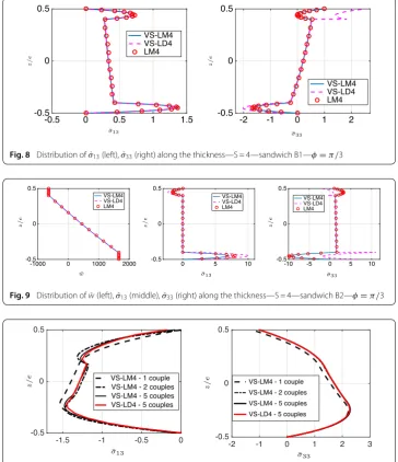
7_{forα = 1 andα = 10}−2_{, respectively. This test case is} dis-criminating for the assessment of composite models. In [83], the authors have shown that LayerWise models are needed to obtain accurate distributions of the transverse stresses through the thickness for this soft core sandwich shell. Moreover, the use of a mixed formulation with an order expansion greater than two, also increases the accuracy of the results. The present approach can be assessed for this discriminating test case. The distributions through the thickness of the transverse displacement and the transverse shear/normal stresses are given in Figs.8 and9. It can be noticed that the results are in very good agreement with the LM4 model. The localisation of the transverse stress in the faces of the sandwich is well-represented. Very high values are reached, contrary to the plate case where the maximum value occurs on the loading surface. The results issued from the VS-LD4 model are also provided for further comparison. For both cases, it shows that the transverse normal stress is very difficult to obtain by a displacement based formulation even with a higher-order theory.

Bending analysis of laminated shells under a constant pressure

Fig. 8 Distribution of ¯σ13(left), ¯σ33(right) along the thickness—S = 4—sandwich B1—φ=π/3

Fig. 9 Distribution of ¯w(left), ¯_σ13(middle), ¯_σ33(right) along the thickness—S = 4—sandwich B2—_φ=π/3

Fig. 10 Distribution of ¯σ13(left), ¯σ33(right) along the thickness—S = 4—three layers—φ=π/2—constant pressure

used. Only the distribution of the transverse shear and normal stresses are given in Fig.10 as these are the most difficult quantities to compute. It can be inferred from this figure that five couples are needed to obtain accurate results. Nevertheless, the convergence rate is higher for the transverse normal stress. For this later, only two couples allow us to recover the load value on the top surface of the shell.

Conclusion