R E S E A R C H A R T I C L E
Open Access
Efficient solvers for time-dependent
problems: a review of IMEX, LATIN,
PARAEXP and PARAREAL algorithms for
heat-type problems with potential use of
approximate exponential integrators and
reduced-order models
Florian De Vuyst
*Correspondence:
[email protected] CMLA, ENS Cachan Université Paris-Saclay, CNRS, 94235 Cachan, France
Abstract
In this paper, we introduce and comment some recent efficient solvers for time dependent partial differential or ordinary differential problems, considering both linear and nonlinear cases. Here “efficient” may have different meanings, for instance a computational complexity which is better than standard time advance schemes as well as a strong parallel efficiency, especially parallel-in-time capability. More than a review, we will try to show the close links between the different approaches and set up a general framework that will allow us to combine the different approaches for more efficiency. As a complementary aspect, we will also discuss ways to include reduced-order models and fast approximate exponential integrators as fast global solvers. For developments and discussion, we will mainly focus on the heat equation, in both linear and nonlinear form.
Keywords: IMEX, LATIN, PARAEXP, PARAREAL, Performance, Reduced order model
Background
This paper deals with efficient numerical approaches to solve time-dependent problems, possibly including parallel-in-time sub-domain decomposition and making help of coarse reduced-order model solvers. As a typical problem of discussion, we will consider the classical heat equation: letbe a bounded domain inRm,m ∈ {2,3}with a Lipschitz-continuous boundary. Letκ be a positive constant. ConsiderT > 0,u0 ∈ H01() and f ∈ L2((0, T), L2()). The linear heat problem with u0 an initial value, homogeneous boundary conditions, for timetin the interval [0, T] reads
⎧ ⎪ ⎨ ⎪ ⎩
∂tu− ∇ ·(κ∇u)=f in×[0, T],
u(., t)=0 on∂×[0, T], u(.,0)=u0 in.
(1)
The problem (1) has a unique solutionuinL2((0, T), H01()). Semi-discretizing the
prob-lem (1) in space (method of lines) will classically lead to a high-dimensional ordinary
©2016 De Vuyst. This article is distributed under the terms of the Creative Commons Attribution 4.0 International License (http:// creativecommons.org/licenses/by/4.0/), which permits unrestricted use, distribution, and reproduction in any medium, provided you give appropriate credit to the original author(s) and the source, provide a link to the Creative Commons license, and indicate if changes were made.
differential problem set inRdwith generally large discrete dimensiond. For simplicity,
we will assume that the semi-discrete problem is written
˙
u+Au=f in [0, T],
u(0)=u0, (2)
withu0 ∈ Rd,f ∈ L2((0, T),Rd) andA ∈ Md(R) typically symmetric positive definite,
with a sparse structure. In this paper we will also consider nonlinear versions of the heat problem with a thermal conductivity coefficientκ(u) depending onuitself. We will assume that there exists a constantκ >0 and a constantκ >0 such that
κ ≤κ(u)≤κ ∀u.
The nonlinear heat problem reads ⎧
⎪ ⎨ ⎪ ⎩
∂tu− ∇ ·(κ(u)∇u)=f in×[0, T],
u(., t)=0 on∂×[0, T], u(.,0)=u0 in
(3)
and we will assume that its semi-discretized form reads
˙
u+A(u)u=f in [0, T],
u(0)=u0
withA(u) sparse, symmetric positive definite for anyu, uniformly bounded. Let us now consider time discretization. Usually, time advance schemes for such kind of problems are chosen implicit or semi-implicit for stability purposes. As an exemple, the pure explicit Euler time advance scheme
un+1−un
t − ∇ ·(κ(u
n)∇un)=f
whereunu(., tn),tn+1=tn+thas a too restrictive numerical stability domain with typicallyt = O(h2),hbeing representative of the space step size. Semi-implicit linear schemes in the form
un+1−un
t − ∇ ·(κ(u
n)∇un+1)= f
show a far better stability domain but require the update of the stiffness matrix with the solution of a large linear sparse system at each time step. Finally, full implicit schemes
un+1−un
t − ∇ ·(κ(u
n+1)∇un+1)= f
The PARAEXP algorithm
Numerical methods allowing parallelization in the time direction have been thought since a long time (see Nievergelt [20] in 1964) and have known great developments particularly in the last decade because of today’s growing HPC platforms. Among time-parallel solvers, the PARAEXP algorithm introduced by Gander and Güttel [10] in 2013 is dedicated to linear ordinary differential problems, that is problems in the form
˙
u+Au=f(t), t∈[0, T],
u(0)=u0 (4)
especially whenf(t) is varying fastly in time. Problem (4) has a solution written in integral form thanks to the variation-of-constant formula:
u(t)=exp(−tA)u0+ t
0
exp(−(t−τ)A)f(τ)dτ. (5)
If we want to take advantage of (5) for deriving a numerical computational method, in particular we need a high-order quadrature formula of the integral term. If thef(t) are fast varying source terms, quadrature may become irrelevant from the accuracy point of view. Gander and Güttel rather propose to split the problem overpsub-domains in time and use a superposition principle based on independent problems set onto different time domains:
1. First, define a partitioning of the time domain [0,T] into p time sub-intervals [Tj−1, Tj],j=1, ..., p, 0=T0<T1<...<Tp=T;
2. For eachj=1, ..., p, solve the initial zero value problem
˙
vj(t)= −Avj(t)+f(t), vj(Tj−1)=0, t∈[Tj−1, Tj]; (6)
3. For eachj=1, ..., p, solve the homogeneous problem
˙
wj(t)= −Awj(t), wj(Tj−1)=vj−1(Tj−1), t∈[Tj−1, T] (7)
(with the notationv0(T0) :=u0).
It is clear that by a superposition principle, on can synthesize a solutionuof (4) by the summation formula
u(t)=vk(t)+
k
j=1
wj(t) forksuch thatt∈[Tk−1, Tk], k∈ {1, ..., p}. (8)
The PARAEXP algorithm is dedicated to parallel computing architectures, otherwise of course there is no benefit to execute it sequentially on one processor. It is remarkable to notice that good implementations of PARAEXP do not require any communication until the solution synthesis step, so the theoretical optimal efficiency is 1 before synthesis. Of course there is an issue of load balancing between processors because for a uniform time domain partitioning, some processors (especially the first one) are doing more work than others. The algorithm is graphically summarized in Fig.1.
Another key of performance is the fast computation of the matrix exponentials. The solution of the homogeneous problem (7) in [Tj−1, T] is
wj(t)=exp(−At)vj−1(Tj−1)
Fig. 1 Schematics of the PARAEXP algorithm [10].Solid red linesrepresent the solutions of inhomogeneous problems with zero initial value on each time slice [Tj−1, Tj], computed in parallel.Blue dashed linesrepresent
the solutions of homogeneous problems on time intervals [Tj, T], also computed in parallel
search approximations into the Krylov subspaceKMof dimensionM: KM =span(u0, Au0,. . ., AM−1u0),
looking for a best approximation into the truncated series expansion. We will come back on this issue when reduced order models (ROM) will be introduced below.
Nonlinear problems: an implicit-explicit IMEX time advance scheme
Hereafter, we switch to the nonlinear case considering the nonlinear heat equation as reference example. Before going into iterative and parallel algorithms, let us first consider a variant implicit-explicit (IMEX) time advance scheme introduced by Filbet, Negulescu and Yang [8] in 2012. The idea is to consider an implicit linear diffusion term with an upper bound of the thermal conductivity, and explicit remainding terms at the right hand side:
un+1−un
t − ∇ ·(κ∇u
n+1)
linear, constant coefficients
= −∇ ·[κ−κ(un)]∇un
varying coefficients, depend onu
+f, (9)
with
κ ≥ sup
x,t κ
(u(x, t)).
As demonstrated in [8], let us show that the semi-discrete in time scheme is stable in the one-dimensional case for a certain norm. Consider the homogeneous case f = 0 with homogeneous Neumann boundary conditions to simplify. We multiply (9) onun+1 on the domain=(0,1), hence we have
1 2
1
0 |u
n+1|2 ds− 1
2 1
0 |u
n|2 ds≤
1
0
(un+1)2−un+1unds ≤t
1
0
(κ−κ(un))∂xun∂xun+1−κ(∂xun+1)2
ds
Let us recall the Peter-Paul inequality (extended Young’s inequality): for any nonnegative real numbersaandb, we haveab≤εa2/2+b2(2ε) for everyε >0. Using the assumption thatκ(un)≤κ, and applying Peter-Paul’s inequality witha= |∂xun|we obtain
(κ−κ(un))∂xun∂xun+1≤ ε2(∂xun)2+
(κ−κ(un))2 2ε (∂xu
n+1)2
≤ ε 2(∂xu
n)2+κ2
2ε(∂xu
Therefore with the choiceε=κ, we have the weighted Sobolev norm decrease
1 2
1
0
(un+1)2dx+κ 2t
1
0 |∂xu
n+1|2dx≤ 1
2 1
0
(un)2dx+ κ 2t
1
0 |∂xu
n|2dx.
This semi-discretization leads to a full discrete scheme in the form
un+1−un
t +Au
n+1=g(un) (10)
with g(u) in the form g(u) = (A−A(u))u+f. What is interesting of course is that the matrix of the implicit part is constant, and thus has to be assembled and factorized once. Moreover the system is linear in the variableun+1. Unfortunately, the PARAEXP algorithm cannot be applied directly here because the right hand sideg(un) depends on the solution itself.
Iterative methods: the LATIN approach
A usual way to deal with nonlinear equations numerically is to use an iterative process within a fixed point algorithm. The LATIN (LArge Time INcremental) method pioneered by Ladevèze [15] and since then broadly used in computational structural Mechanics and material science (see [16] for a recent reference) solves time-dependent problems (linear or nonlinear) according to a two-step iterative process. To separate the difficulties, equa-tions are partitioned into two groups: (i) a group of equaequa-tions being local in space and time, possibly nonlinear (representing equilibrium equations for example); (ii) a group of linear equations, possibly global in the spatial variable. Then ad-hoc space-time approximations methods are used for the treatment of the global problem. Of course, space-time local equations can be solved in parallel, what makes the LATIN method efficient and suitable for today’s HPC facilities. Let us emphasize that with LATIN, it is possible to solve hard nonlinear mechanics problems including thermodynamics irreversible problems (plastic-ity, friction as examples).
As an llustration, let us describe the LATIN method on the (rather simple) nonlinear heat problem:
1. Initialization (k=0): letu(0)∈L2((0, T), H1()) an approximate solution (in space
and time) of the nonlinear problem (it can be an approximate solution obtained with a coarse solver for example); compute ˜κ(0)=κ(u(0));
2. Iteratek, step 1 (global linear solution). Solve the linear problem
∂tu(k+1)− ∇ ·(˜κ(k)∇u(k+1))=f
with given initial and boundary conditions.
3. Iteratek, step 2 (local projection over the admissible manifold). Compute
˜
κ(k+1)=κ(u(k+1)).
4. Check convergence,k←k+1 if not and go to 2.
The step 1 performs a global (linear) evolution of the solution whereas a pointwise nonlinear projection on the equilibrium conductivity coefficients is done in step 2. We have a natural convergence indicator in terms of distance between the frozen conductivity
˜
e(k)=κ(u(k+1))−κ˜(k).
In particular, ifκis Lipschitz continuous with Lipschitz constantL, then
e(k)≤L u(k+1)−u(k) .
Remark that step 2 can be performed in parallel (in time).
For better and faster convergence, one can imagine variant approaches using a relaxation approach: remark first thatκ(u) is (formally) solution of the partial differential equation
∂tκ(u)− ∇ ·(κ(u)∇κ(u))=κ(u)f −κ(u)κ(u)|∇u2|.
Ifκis a strictly convex function for example, then the second term at the right hand side is negative. One may consider the approximate (augmented) problem
⎧ ⎨ ⎩
∂tu− ∇ ·(˜κ∇u)=f,
∂tκ˜− ∇ ·(κ∇κ˜)=κ(u)f + κ
(u)−κ˜
ε .
(11)
where ε > 0 is a given relaxation time (assumed to be rather small). By this way, it is expected that ˜κ evolves much closer toward the valueκ(u). One can then derive an iterative process with again two steps (linear solution +projection) as in the LATIN method.
Newton and quasi-Newton approaches
For the sake of simplicity, let us consider here the initial value problem with general autonomous system of ordinary differential equations
˙
u=f(u), t∈(0, T], (12)
withfassumed to be differentiable and Lipschitz continuous, and initial conditionu(0)= u0. The solutionu∈L2((0, T),Rd) can be seen as the zero of a nonlinear operatorG,
G(u) :=u˙−f(u)=0.
The directional derivative ofGat pointuin the directionvis
DG(u)v=v˙−Df(u)v.
Then the standard Newton-Raphson method applied toGreads for thek-th iterate
DG(u(k))(u(k+1)−u(k))= −G(u(k))
that simplifies into
˙
u(k+1)=f(u(k))+Df(u(k))(u(k+1)−u(k)) =Df(u(k))u(k+1)+
f(u(k))−Df(u(k))u(k)
(13)
Hence, the Newton-Raphson method provides a sequence of linear problems (of unknown u(k+1)) with variable coefficients and sources (depending onf andu(k)).
Spectral structure of the linearized problem
Let us emphasize that, at a givenk, the linear system has the expected spectral structure for approximate solutions near an equilibriumu, that isf(u)= 0. Foru(k+1)close tou, we have
d
dt(u(k+1)−u)=Df(u(k))(u(k+1)−u)+
f(u(k))−f(u)−Df(u(k))(u(k)−u)
Foru(k)close touandf ∈C2we have
f(u(k))−f(u)−Df(u(k))(u(k)−u)=O(|u(k)−u|2),
then d
dt(u(k+1)−u)Df(u)(u(k+1)−u) which is the expected linearized system.
Quasi-Newton approach
As an additional approximation, a quasi-Newton method will replace the Jacobian matrix Df(uk) by an approximate oneA(k)Df(uk), simpler to compute, thus giving the iterative
process
˙
u(k+1)=f(u(k))+A(k)(u(k+1)−u(k))
=A(k)u(k+1)+
f(u(k))−A(k)u(k)
If we are able to build some coarse approximationgoff such that the quasi-Newton secant condition
A(k)(u(k+1)−u(k))=g(u(k+1))−g(u(k)) (14)
is satisfied, we get the Jacobian-free quasi-Newton iteration
˙
u(k+1)=f(u(k))+
g(u(k+1))−g(u(k))
(15)
or equivalently
˙
u(k+1)=g(u(k+1))+
f
(u(k))−g(u(k))
. (16)
In (16),g(u(k+1)) can be seen as a predictor term, whereas (f(u(k))−g(u(k))) is a corrector
term towardf depending on the iterate (k) only. By construction we retrieve the accuracy off at convergence. A quasi-Newton secant condition ensures superlinear convergence according to the Dennis and Moré theorem.
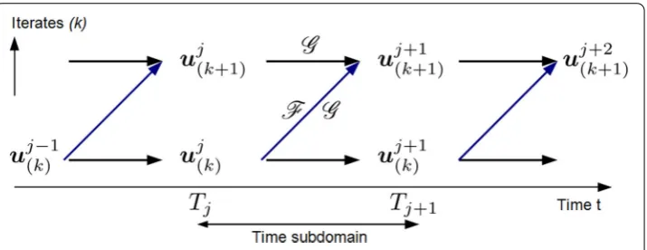
The PARAREAL method
The recent PARAREAL method, initially proposed by Lions et al. [17] in 2001, is nothing else but a parallel-in-time version of the quasi-Newton method (16) above. In PARAREAL, the time domain is decomposed into p subdomains. Then we define a double-index sequence of approximate solutionsuj(k), wherek still denotes the current index of the iterative process and j is the number of the time subdomain [Tj−1, Tj]. In its regular
current form (see [3,4]), the PARAREAL algorithm is defined as follows:
1. Define a partition in time [Tj−1, Tj], 0=T0<T1<...<Tp=T;
2. Define a cheap coarse propagatorG and a fine propagatorF. 3. Initialization (k=0):u0
(0)=u0,u
j+1 (0) =G(u
j
(0));
4. Loop on the iteratesk:
uj+1
(k+1)=G(u
j
(k+1)) +
F(uj(k))−G(uj(k)) (17) 5. Check convergence, test the stop criterion.
Fig. 2 Schematics and graph dependency into the PARAREAL algorithm
F(uj(k))−G(uj(k))
can be evaluated in parallel over thepprocessors. On the other hand the coarse propagator termG(uj(k+1)) induces a persistent sequential part into the algorithm but it is expected to be evaluated quite fast. The trade-off is to design a fast, “accurate enough” coarse propagator which does not affect the whole performance of the algorithm.
One can imagine different choices of coarse solvers: low-order accurate time advances schemes, simplified equations, simplified models, discretizations on coarser meshes, etc. Reference papers like Bal and Maday [4] and Baffico et al. [3] show general convergence theorems for nonlinear ordinary differential systems using coarse time integrators as coarse solvers. Gander and Hairer in [9] also show a superlinear convergence of the parareal algorithm.
Putting all together
Actually, there are different ways to mix the strategies seen so far. As an example, let us still consider the nonlinear heat equation with time-varying source term:
∂tu− ∇ ·(κ(u)∇u)=f(t).
In the spirit of IMEX and LATIN, let us define the following iterative approach:
∂tu(k+1)− ∇ ·(κ∇u(k+1))=f(t)+ ∇ ·((κ−κ(k))∇u(k)), (18)
κ(k+1)=κ(u(k+1)). (19)
On the left-hand side of the equation, we have replaced the thermal conductivityκ(u) by some supremum as suggested by IMEX. In semi-discrete form, we get an equation in the form
˙
u(k+1)+Au(k+1)=f(t)+r(k). (20)
We get a linear equation for the unknownu(k+1)with constant coefficient matrixA, and
the right hand side only depends on time throughf(t) andu(k)(t). Then the PARAEXP
algorithm can be applied at each iterativek. The remaining nonlinear operations like (19) and the assembling ofr(k)can be done in parallel (in time). In conclusion, we have replaced
The Newton method to handle nonlinear terms with ROMs of dynamical systems
Reduced-order modeling is a general methodology to determine the principal information of a general high-dimensional problem and then reduce the problem, for example by projection. Reduction is generally possible when theM-Kolmogorov width
δM(U)= inf
VMlinear space, VM⊂V dim(VM)=M
sup
x∈U
inf
yM∈VM x−y
M V.
into an admissible close set U of a Banach spaceV is rather small for a rather small integer M(the dimension of the approximate space). One of the main motivations to do that is to strongly reduce the computational cost for the numerical solution. Even if there are recent advances in nonlinear reduced order modeling, in particular with the empirical interpolation method (EIM) proposed by Maday et al. [18], or discrete empirical interpolation method (DEIM) by Chaturantabut and Sorensen [5], there are still some issues and open problems for nonlinear time-dependent problems. Dealing with general nonlinear terms and reduced-order modeling for dynamical systems may be a difficult task, because:
• reduced-order models are expected to reproduce the stability of the system (for instance in the sense of Lyapunov, see [14] on this subject);
• the local dynamics has to be reproduced, at least “at first order”, involving a compat-ibility of the spectral properties between full and reduced systems;
• the area visited by the trajectories into the state-space may be defined over a nonlinear manifold rather than in a linear subspace. Thus nonlinear dimensionality reduction methods would be better candidates for reduction.
Balanced truncation strategy [1,22] for example is a trade-off in the reduction process to provide sufficient accuracy for controllability and observability of dynamical systems. However the theory mainly deals with linear time-invariant (LTI) systems.
For time-dependent problems, one can adopt a greedy incremental strategy during time by adapting/enriching the low-dimensional subspace when the principal components are changing during time. But the price to pay is to online evaluate some (high-dimensional) nonlinear terms to control the error, what can be a penalizing factor of performance. If there is no other choice, parallel-in-time computing once again appears to be a comple-mentary tool to keep global performance of the method.
Newton method and Galerkin projection method
Let us go back to the Newton method (13) that we rewrite here again
˙
u(k+1)=Df(u(k))u(k+1)+f(u(k))−Df(u(k))u(k).
Let us consider a Galerkin approximation into the linear vector space
V(Mk)=span(w1(k),. . .,wM(k))
and assume that (w(k),wm(k)) = δm, 1 ≤ , m≤ M. We are looking for an approximate rank-MsolutionuMk+1(t) inV(Mk), i.e.
uM
(k+1)(t)=
M
m=1
for some real coefficientsam
(k+1)(t), 1≤m≤Mat timet. In order to get a reduced system,
the Eq. (13) is projected onto the vector spaceV(Mk). Multipling (13) by any test function vM ∈VM
(k), we look for a low-order solutionuM(k+1)(t) in the form (21) such that
˙ uM
(k+1),vM
=Df(u(k))uM(k+1),vM
+f(u(k))−Df(u(k))u(k),vM
, ∀vM ∈V(Mk).
TakingvM =wm(k), 1≤m≤M, by orthogonality of the eigenvectors we get
˙ am(k+1)=
M
=1
a(k+1)(Df(u(k))w(k),wm(k))+(f(u(k))−Df(u(k))u(k),wm(k)).
In vector form, one obtains a reduced system in the form
˙ aM
(k+1)=A˜M(k)(t)aM(k+1)+rM(k)(t)
with aM(k+1)(t) = (am(k+1)(t))m, ( ˜AM(k))m(t) = (Df(u(k)(t))w(k),wm(k)) and (rM(k)(t))m =
(f(u(k)(t))− Df(u(k)(t))u(k),wm(k)). Remark that when the initial system is linear, i.e.
f(u)=Au, we retrieve the classical Galerkin projection over the spaceVM: ˙
aM
(k+1)=A˜(Mk)aM(k+1)
with a constant matrix ˜AM(k), ( ˜A(Mk))m = (Aw(k),wm(k)). The assembling of both ˜AM(k)(t) andrM(k)(t) requires high-dimensional operations, but, fortunately, one can do this task in parallel (in time). Thus, one can nonetheless expect to get rather high performance. To summarize, at this stage of analysis, the algorithm of reduced-order modeling is the following:
1. (initialization). Use a coarse solver and computeu(0). Loop over (k):
2. ComputeMprincipal componentswm(k),m= 1,. . ., Mor a suitable reduced basis from the knowledge ofu(k).
3. Assemble and compute in parallel ˜AM
(k)(t) andrM(k)(t) at all the discrete times.
4. Solve the linear problem
˙ aM
(k+1)=A˜(Mk)(t)aM(k+1)+rM(k)(t), t∈(0, T]
aM
(k+1)(0)=a0(k+1) ∈RM,
and compute
uM
(k+1)(t)=
M
m=1
am(k+1)(t)wm(k). 5. Test convergence after iteratek.
Remark 1 For the computation of the basis functionswm(k), one can of course use Proper Orthogonal Decomposition (POD) [22] or any other dimensionality reduction method. The update the reduced basis may also be done by incrementing the basis set within an adaptive learning algorithm.
Remark 2 In the step 3, it is assumed that both ˜A(k)(t) andr(k)(t) have to be assembled
Discussion about further reduction
There are many options to improve the whole numerical complexity of the algorithm using some additional approximations or reduction strategies.
Freezing up the Jacobian matrices Let us go back to the Newton method
˙
u(k+1)=f(u(k))+Df(u(k))(u(k+1)−u(k))
where the correction termDf(u(k))(u(k+1)−u(k)) ensures quadratic convergence when it is converges. As already discussed in “Newton and quasi-Newton approaches”, one can approximate the Jacobian matrix by some approximationA(k)(t) which is cheaper to
evaluate, leading to the quasi-Newton approach
˙
u(k+1)=f(u(k))+A(k)(t) (u(k+1)−u(k)).
The matricesA(k)still depend on timeta priori. But one could consider frozen
approxi-mates Jacobian matricesAj(k)of time slices [Tj, Tj+1], further inviting for a parallel-in-time
strategy.
Adding coarse models
If we do not want to worry about Jacobian matrices, then the other option is to consider a coarse modelgoff as mentioned in “Newton and quasi-Newton approaches” section. In this case, the quasi-Newton iteration reads
˙
u(k+1)=f(u(k))+
g(u(k+1))−g(u(k))
.
In order to achieve an efficient reduced-order model, one have now to deal with the nonlinear termg(u(k+1)). An efficient and tractable way to proceed is to use an empirical
interpolation method (EIM, [18]) for that. In that case, we can even makeg depend on (k), according to some adaptive learning process (greedy algorithm, inflating basis, etc). Remark finally that the iterative process can once again be set up into a parallel-in-time framework following ideas from the PARAREAL algorithm.
Achieving dimensionality reduction forf
If possible, one can also use a reduced-order approximation forf. If the iterative algorithm is expected to converge towards a solution that has the same order of accuracy than the original one, one have to consider an accurate reduced-order model for f. Once the empirical interpolation method may help us for that. However, if a global-in-time reduction strategy is considered, it is possible that the dimension Mof the low-order vector space becomes too large, leading to a degradation of the whole performance.
An alternative approach would be to consider a family of local-in-time empirical inter-polation methods forf. In this case, we should also consider local modelsfj(k)available in the time slice [Tj, Tj+1[ which can also be updated at eachkfrom a learning process.
Approximate exponential integrators
precisely, for the the problem ˙u=Auwith initial datau(0)=u0, we have to compute the
solutionu(t)=exp(tA)u0for anyt∈[0, T].
As mentioned in [9], there are numerous techniques to determine accurate exponential matrices. Among then, one can for example mention Padé approximants, exponentially fitted integration methods, or approximations based on projections over Krylov subspaces
KM =[u0Au0A2u0 . . . (AM−1u0)].
through Arnoldi orthogonalization iterations [12]. Actually the Krylov-Galerkin projec-tion can be seen as a reduced-order technique, with a suitable reduced basis that fits acprojec-tion of matrix exponentials. But of course there are other choices of suitable basis functions like the first eigenvectorsφmofA:
Aφm=λmφm.
ForAsymmetric positive definite with eigenvalues arranged in increasing order, that is 0< λ1≤λ2≤. . . λM≤. . ., it is natural to consider from the approximation error point
of view theM first eigenvectors of Aas vectors spanning the reduced approximation subspace. We will denote ˜Athe projection ofAon this discrete subspace and of course we have rank(A)=M. Considering the iterative approach of linear problems
˙
u(k+1)=A˜u(k)+(A−A˜)u(k), t∈[0, T], (22)
u(0)=u0, (23)
by superposition principle, one can first consider the low-order homogeneous problem
˙
v(k+1) =A˜v(
k+1),
v(k+1)(0)=u0
for which we have an efficient low-order exponential solution, and on the other side the high-dimensional problem with zero initial value
˙
w(k+1)=A˜w(
k+1)+(A−A˜)u(k),
w(k+1)(0)=0,
then u(k+1)(t) = v(k+1)(t)+w(k+1)(t). In the spirit of the PARAEXP algorithm, one can set up the superposition principle within a parallel-in-time time decomposition to deal separately with low-order homogeneous exponential solution and high-dimensional inhomogeneous problems.
Closing discussion
From this review on efficient time-advance solvers including IMEX, LATIN, PARAEXP and PARAREAL algorithms, we try to show the different ways and tracks to deal with large-scale dynamical systems, linear and/or nonlinear terms. For the sake of an easy discussion, we have taken the example of the heat equation (linear or nonlinear). We are aware that this may be too restrictive and nonlinear computational mechanics including for example thermodynamics irreversible problems need more efforts and technical developments. Among the methods discussed above, some of them have been designed to address these problems. This is the case for the LATIN approach for example.
methodology to accelerate the whole time advance solution. For numerous reasons, it is interesting to cast a nonlinear problem into a sequence of linear problems within an iter-ative process. Linear problems are easier to deal with, and there are dedicated tools like the parallel-in-time PARAEXP method. On the other hand, an iterative process allows for achieving multi-fidelity adaptive solvers, using incremental, greedy or learning algorithms. Of course, we have to keep in mind that iterative methods may not converge. So in the design process of the numerical approach, one has to answer to the following questions: is the whole iterative process stable, is it possible to prove the convergence ? If the method is convergent, what is the rate of convergence ? Is it possible to accelerate the convergence ? At convergence, is it sure that the iterative algorithm converges to the solution obtaines with the accuracy we paid at the finest level ? For parallel algorithms, what is the effective speedup ?
Last but not least, managing multi-fidelity models and multi-level reduced-order models as well as parallel-in-time algorithms and learning algorithms implemented on distributed memory computer architecture necessarily require data management efforts and smart software engineering.
Conclusions
The first aim of this paper is to review different efficient time-advance solvers (including IMEX, PARAEXP, LATIN, PARAREAL) and show connections between them. We also try to show the links with quasi-Newton approaches and relaxation/projection methods to deal with nonlinear terms. Parallel-in-time algorithms appear to be a complemen-tary and promising framework for the fast solution of time-dependent problems. Finally, reduced-order models (POD-based, principal eigenstructure, a priori reduced bases, ...) can be possibly included to achieve better performance. In a future paper, we will achieve numerical experiments on different hybrid approaches.
Received: 13 November 2015 Accepted: 2 March 2016
References
1. Antoulas AC. An overview of approximation methods for large-scale dynamical systems. Annu Rev Control. 2005;29:181–90.
2. Audouze C, De Vuyst F, Nair PB. Nonintrusive reduced-order modeling of parametrized time-dependent partial differential equations. Numeri Methods Partial Differen Equ. 2013;29(5):1587–628.
3. Baffico L, Bernard S, Maday Y, Turinici G, Zrah G. Parallel-in-time molecular dynamics simulations. Phys Rev E. 2002;66(5):057701.
4. Bal G, Maday Y. A “parareal” time discretization for nonlinear PDEs with application to the pricing of an American put. Recent developments in domain decomposition methods. Berlin: Springer; 2002. p. 189–202.
5. Chaturantabut S, Sorensen DC. Nonlinear model reduction via discrete empirical interpolation. SIAM J Sci Comput. 2010;32(5):2737–64.
6. Chinesta F, Ammar A, Lemarchand F, Beauchène P, Boust F. Parallel time integration and high resolution homoge-nization. CMAME. 2008;197(5):400–13.
7. Cortial J, Fahrat C, Guibas LJ, Rajashekhar M. Compressed sensing and time-parallel reduced-order modeling of structural health monitoring using DDDAS. Computational science-ICCS 2007. Berlin: Springer; 2007. p. 1171–9. 8. Filbet F, Negulescu C, Yang C. Numerical study of a nonlinear heat equation for plasma Physics. Int J Comp Math.
2012;89(8):1060–82.
9. Gander MJ, Hairer E. Nonlinear convergence analysis for the PARAREAL algorithm. In: Domain decomposition methods in Science and Engineering. 2008. vol. 60, p. 4556.
10. Gander MJ, Güttel S. PARAEXP: a parallel integrator for linear initial-value problems. SIAM J Sci Comput. 2013;35(2):C123–42.
11. Gander MJ. 50 years of time parallel time integration. Multiple shooting and time domain decomposition. Berlin: Springer; 2015.
13. Kalashnikova I, Barone MF. On the stability of a Galerkin reduced order model (ROM) of compressible flow with solid wall and far-field boundary treatment. IJNME. 2010;83:1345–75.
14. Kalashnikova I, Barone MF, Arunajatesan S, von Bloemen Waanders BG. Construction of energy-stable projection-based reduced order models. Appl Math Comp. 2014;249:569–96.
15. Ladevèze P. Non linear computational structural mechanics new approaches and non-incremental methods of calculation. New York: Springer-Verlag; 1999.
16. Ladevèze P, Passieux JC, Néron D. The LATIN multiscale computational method and the proper generalized decom-position. Comput Methods Appl Mech Eng. 2010;199(21):1287–96.
17. Lions J, Maday Y, Turinici G. A “parareal” in time discretization of PDE’s. Comptes Rendus de l’Académie des Sciences, Séries I, Mathematics. 2001;332(7):661–8.
18. Maday Y, Nguyen NC, Patera AT, Pau GSH. A general multipurpose interpolation procedure: the magic points. Commun Pure Appl Anal. 2009;81:383–404.
19. Minion M. A hybrid parareal spectral deferred corrections method. Commun Appl Math Comput Sci. 2010;5(2):265– 301.
20. Nievergelt J. Parallel methods for integrating ordinary differential equations. Comm ACM. 1964;7:731–3.
21. Prud’homme C, Rovas D, Veroy K, Maday Y, Patera AT, Turinici G. Reliable real time solution of parametrized partial differential equations: reduced-basis output bound methods. J Fluids Eng. 2002;124(1):70–80.
![Fig. 1 Schematics of the PARAEXP algorithm [10]. Solid red lines represent the solutions of inhomogeneousproblems with zero initial value on each time slice [Tj−1, Tj], computed in parallel](https://thumb-us.123doks.com/thumbv2/123dok_us/9583621.1941095/4.595.117.478.86.183/schematics-paraexp-algorithm-represent-solutions-inhomogeneousproblems-computed-parallel.webp)