www.adv-radio-sci.net/13/161/2015/ doi:10.5194/ars-13-161-2015
© Author(s) 2015. CC Attribution 3.0 License.
Application of transmission-line super theory to classical
transmission lines with risers
R. Rambousky1, J. Nitsch2, and S. Tkachenko2
1Bundeswehr Research Institute for Protective Technologies and NBC Protection (WIS), Munster, Germany 2Otto-von-Guericke University Magdeburg, Magdeburg, Germany
Correspondence to: R. Rambousky ([email protected])
Received: 5 November 2014 – Revised: 22 April 2015 – Accepted: 4 May 2015 – Published: 3 November 2015
Abstract. By applying the Transmission-Line Super Theory (TLST) to a practical transmission-line configuration (two risers and a horizontal part of the line parallel to the ground plane) it is elaborated under which physical and geometrical conditions the horizontal part of the transmission-line can be represented by a classical telegrapher equation with a suffi-ciently accurate description of the physical properties of the line. The risers together with the part of the horizontal line close to them are treated as separate lines using the TLST. Novel frequency and local dependent reflection coefficients are introduced to take into account the action of the bends and their radiation. They can be derived from the matrizant elements of the TLST solution. It is shown that the solution of the resulting network and the TLST solution of the en-tire line agree for certain line configurations. The physical and geometrical parameters for these corresponding configu-rations are determined in this paper.
1 Introduction
Transmission-Line Super Theory (TLST) was introduced by Haase and Nitsch (2001, 2003) more than one decade ago. In this theory Maxwell’s equations are represented for a tem of lossless nonuniform thin transmission lines in a sys-tem of equations which have the same structure as the tele-grapher equations. In particular, the TLST equations take into account all field modes and physical effects that might occur, including radiation losses. It surpasses the classical transmission-line theory, which is a special case. Their com-plex parameters are local and frequency dependent and are obtained by the solution of integral equations.
In the paper a practical classical transmission-line (cTL) is regarded. The considered TL consists of a finite part parallel to the ground plane and two vertical risers connecting the horizontal part to the conducting ground plane at the ends.
In Sect. 2 the classical analysis of the TL is briefly de-scribed and the classical reflection coefficients are intro-duced. In Sect. 3 the fundamentals of TLST are presented and the finite transmission line with risers is analyzed using the numerical TLST procedure. The local and frequency de-pendent parameter matrix elements representing the per unit length inductance and capacitance values are discussed. A procedure is shown where the whole TL can be separated in uniform and nonuniform parts. Only for the nonuniform parts TLST has to be used and the asymptotic part can be handled classically. In Sect. 4 novel local and frequency de-pendent reflection coefficients are introduced and it is shown how they are related to the matrizant elements of the TLST. Finally it is shown how the current on the TL can be calcu-lated using the reflection coefficients. Numerical results for the finite uniform TL with risers are shown and discussed in Sect. 5. Calculated results for the novel reflection coefficients and current values on the TL are shown for several geomet-rical constitutions of the TL. Finally the results are discussed and summarized in Sect. 6.
2 A finite TL in classical transmission-line theory
dU (z) dz +j ωL
0
cTLI (z)=0
dI (z) dz +j ωC
0
cTLU (z)=0, (1)
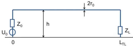
wherez is the axial orientation of the TL (see Fig. 1) and
U (z)andI (z)are the complex voltage and current distribu-tions on the line. The classical (and constant) per unit length (p.u.l) inductance and capacitance are named as L0cTL and
CcTL0 , respectively.
The finite classical TL with risers over a conducting ground plane (PEC) regarded in this work is shown in Fig. 1. To simplify the presentation the following parameters for the TL are chosen, although the outlined method works in gen-eral: wire radiusr0=0.5 mm; height over groundh=5 cm; length of the horizontal partLTL=2 m; total arc length of the TLL=LTL+2h=2.1 m. At the beginning the line is fed by a lumped source with voltage U0=1 V and source impedance Z0=50. The line is terminated with a load impedanceZL=50. The formulas for the classical p.u.l. inductanceL0cTLand capacitanceCcTL0 are
L0cTL=µ0
2πln
2h
r0
=1.06×10⁻⁶V s
A m (2)
CcTL0 = 2π 0
ln2hr 0
=1.05×10 −11 A s
V m, (3)
resulting in a characteristic line impedance of ZC= q
L0cTLC0−1cTL=318.
A current wave originating at+∞, traveling on the hori-zontal part of the TL in−zdirection and being reflected at the beginning of the TL atz=0 can be expressed using the classical left-hand current reflection coefficientRclass+ as
I (z)=I1
ej kz+R+classe−j kz. (4) withI1being an appropriate constant. From Eq. (1) the ex-pression for the voltageU (z)= − 1
j ωC0dI (z)dz can be deduced and together with Eq. (4) the result for the left-hand current reflection coefficient is calculated as
R+class=e2j kzZCI (z)+U (z) ZCI (z)−U (z)
=ZC−Z0
ZC+Z0
. (5)
R−class=e−2j k(z−LTL)ZCI (z)−U (z) ZCI (z)+U (z)
=ZC−ZL
ZC+ZL
. (7)
3 TLST analysis of a finite TL with risers 3.1 Fundamentals of TLST
Transmission-line super theory (Haase and Nitsch, 2001; Haase et al., 2003; Haase, 2005; Nitsch et al., 2009; Nitsch and Tkachenko, 2010) is a full wave description of Maxwell’s equations cast into the form of telegrapher’s equa-tions. For a single wire system (with return conductor or ground plane) the super theory transmission-line equation for lumped sources or loads at the line ends in the potential-current representation states (Rambousky et al., 2012)
∂ ∂l
ϕ(l, f ) i(l, f )
+j ωP∗(1)(l, f )
ϕ(l, f ) i(l, f )
=
0 0
. (8)
The potential on the transmission-line is denoted byϕ(l, f )
and the current byi(l, f ). The best choice for the line pa-rameter is the (natural) arc lengthl of the line andf is the frequency. The super matrix P∗(1)is the transmission-line pa-rameter matrix. In the case of a one wire system P∗(1)is a 2 by 2 matrix. In contrast to cTLT the transmission-line pa-rameter matrix P∗(1)(l, f )now is complex valued and both local (l) and frequency (f) dependent. This parameter matrix is calculated by an iteration process starting with a low fre-quency approximation in the zeroth iteration step resulting in a frequency independent but already local parameter matrix P∗(0)(l)(Nitsch et al., 2009; Rambousky et al., 2012). In pre-vious work we could show that already the first iteration step results in an acceptable accuracy (Rambousky et al., 2013a). The general solution of the super theory transmission-line equation (8) for the one wire case can be written as
ϕ(l, f ) i(l, f )
=Mll 0
n
−j ωP∗(1)o
ϕ(l0, f )
i(l0, f )
, (9)
where the expressionMl
Figure 2. Parameter matrix elements representing the real part of the p.u.l. inductance for TLST analysis of the TL configuration.
Figure 3. Parameter matrix elements representing the imaginary part of the p.u.l inductance for TLST analysis of the TL configu-ration.
sources or lumped loads at the ends of the wires, Eq. (9) can be calculated using the appropriate boundary conditions of the TL model.
3.2 TLST parameter elements for a finite TL with risers
The parameter matrices P∗(0)(l) and P∗(1)(l, f ) resulting from the TLST iteration process are independent of the lumped sources and loads. The P∗
12elements representing the p.u.l. inductance are shown in Fig. 2 (real part) and in Fig. 3 (imaginary part).
Figure 2 indicates that in the TLST the classical p.u.l. in-ductanceL0cTLis reached at a certain distance away from the risers for the configuration presented in Fig. 1. The graph of the inductance bends when approaching the ends of the hor-izontal part of the line and reaches its minima at the ends of the horizontal parts. A reason for this behavior can be found in Nitsch et al. (2009). When passing through the risers it
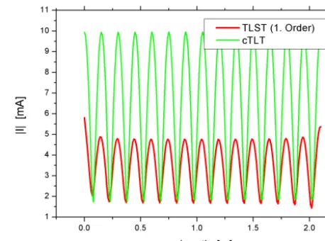
in-Figure 4. Current on the TL calculated using TLST approach for
f=1 GHz compared to classical TL theory.
creases again. Also the imaginary part ofL0deviates signifi-cantly from the classical value (zero) at the risers, indicating the most radiative parts of the TL.
The current on the TL calculated using TLST with first order iteration parameter matrix is shown in Fig. 4 for a fre-quency of 1 GHz. To have a comparable arc length, the total length of the classical TL was also set to 2.1 m. It is clearly seen that the real current distribution deviates significantly from the classical theory, mainly because of the radiating losses at the used frequency.
3.3 Decomposition of the TL based on the group property of the matrizant
In the example of Fig. 1 the TL can be decomposed in the left-hand riser part, the uniform middle part (asymptotic re-gion) and the right-hand riser part. Attention has to be paid that the junctions are located where the composed TL shows almost classical behavior (see Fig. 2). Therefore the junctions have to be sufficiently far away from the riser, like atz1and
z2 as shown in Fig. 5. Now, the TLST parameter matrices for the single parts of the decomposed TL can be calculated. Because even the tail end of an otherwise classical TL shows significant deviation of the line parameters in TLST, the ele-ments of the parameter matrix have to be adjusted due to the junction. For the used TL with risers the asymptotic region (part II) was defined as a classical TL with constant line pa-rameters using Eqs. (2) and (3). The riser parts I and III were adjusted for the junctions by hand to ignore the tail ends and to meet the classical values at the junctions. This is shown in Fig. 6 with the dashed curves.
Figure 6. Real part of the parameter matrix elementP∗(1)12 for the defined three parts of the nonuniform TL and their manual adjust-ment at the junctions.
order parameter matrix P∗(1)
ϕ(L) i(L)
=ML0n−j ωP∗(1)o
ϕ(0) i(0)
=ML
ϕ(0) i(0)
. (10) The matrix MLis the matrizant over the whole arc length of the TL using the parameter matrix P∗(1)of the whole TL.
On the other hand, current and potential in the loadZLcan be calculated using the matrizants MmanI , MmanII and MmanIII of the single parts I, II and III of the TL with the manually (at the junctions) adapted parameter matrices as
ϕ(L) i(L)
=MmanIII ·MmanII ·MmanI
ϕ(0) i(0)
. (11)
For example MmanI is the matrizant covering the arc length froml=0 tol=z1+h=0.6 m using the manually (at the junction) adapted first order parameter matrix P∗(1)I,man result-ing in
MmanI =Mz1+h 0
n
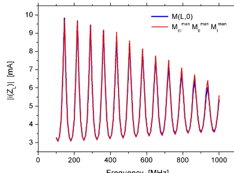
−j ωP∗(1)I,mano. (12) To validate the equivalence of Eqs. (10) and (11) the current inZLat the end of the TL was calculated in both ways. The result is shown in Fig. 7 and gives very good agreement. It
Figure 7. Current in the loadZLat the end of the TL of Fig. 1.
has to be mentioned again that in the assembled solution the middle part (part II) of the TL was regarded as a pure clas-sical TL. The results so far show that the current distribution on a real TL with risers can be calculated by dividing the line in uniform and nonuniform parts. The nonuniform parts have to be calculated using an advanced TLT, like TLST. The uniform parts can be handled as classical TL. The overall ma-trizant of the TL can be assembled by multiplying the single matrizants of the TL parts in correct order.
4 Novel local and frequency dependent current reflection coefficients and amplitude functions The idea now is to transfer the concept of current reflection coefficients from cTLT to a realistic finite transmission-line with risers at both ends.
4.1 Derivation of the novel current reflection coefficients using TLST
In TLST voltageU (z)is replaced by the potentialϕ(l)and current I (z) by i(l). Again l is the natural parameter of the TL (arc length) including the risers. As an extension of Eqs. (5) and (7) the nowl and frequency dependent current reflection coefficients can also be defined as the quotient of an incoming and outgoing current wave as
e
R+(l):=e2j kl
ZCi(l)+ϕ(l)
ZCi(l)−ϕ(l)
(13) and
e
R−(l):=e−2j k(l−L)
ZCi(l)−ϕ(l)
ZCi(l)+ϕ(l)
. (14)
Figure 8. Transmission-line configuration for derivation of the right-hand current reflection coefficientR−(l)e of the TL with
ris-ers.
Sect. 3.3), the matrizant of the whole TL can be composed as a matrix product of matrizants representing parts of the TL. Therefore, actually only the riser parts I and III have to be calculated using TLST and the classical matrizant can be used for the asymptotic region (part II). A theoretical restric-tion for our approach is that no radiarestric-tion coupling between the two riser parts of the TL is allowed. This is assured if the horizontal lengthLTLof the TL is large compared to the heighthover ground.
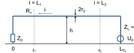
4.1.1 The right-hand reflection coefficientRe−(l)
In Fig. 8 the TL configuration for derivation of the right-hand current reflection coefficient R−(l) is depicted. Imagine a current wave coming from −∞travels in positive z direc-tion, gets reflected at the right-hand riser and travels back to
−∞. The classical telegrapher’s equations are valid in the asymptotic region, defined by L1≤l≤L2. The matrizant Ml
L n
−j ωP∗(1)o≡M(l, L)can be decomposed in
M(l, L)=M(l, L2)·M(L2, L), (15) where the second factor on the right side of Eq. (15) is inde-pendent ofl. Theldependence is restricted to the asymptotic region. ForLTLhthe radiation coupling is negligible and
e
R−(l)is independent ofRe+(l).
In a next step the quotient in Eq. (14) has to be expressed by matrizants of the TLST calculation. Generally the relation
ϕ(l2)
i(l2)
=M(l2, l1)
ϕ(l1)
i(l1)
∀l1, l2∈ [0, L] (16)
holds. Settingl2=landl1=Land using the boundary con-dition ϕ(L)=UL=ZLi(L) the potential-current vector at arc lengthlcan be expressed as
ϕ(l) i(l)
=M(l, L)
ϕ(L) i(L)
=i(L)
M11(l, L) M12(l, L) M21(l, L) M22(l, L)
·
ZL 1
. (17)
Figure 9. Transmission-line configuration for derivation of the left-hand current reflection coefficientR+(l)e of the TL with risers.
Inserting the results forϕ(l)andi(l)in Eq. (14) leads to the advanced expression for the right-hand current reflection co-efficientRe−(l)which is now local and frequency dependent. e
R−(l)=e−2j k(l−L)
·(ZL[−M11(l, L)+ZCM21(l, L)]
+(−M12(l, L)+ZCM22(l, L)))
·(ZL[M11(l, L)+ZCM21(l, L)]
+M12(l, L)+ZCM22(l, L))−1. (18) 4.1.2 The left-hand reflection coefficientRe+(l)
The TL configuration for the derivation ofRe+(l)is depicted in Fig. 9. It is assumed that a current wave traveling in−z
direction gets reflected at the left-hand side of the TL. Using the same concept as before the matrizant can be decomposed in a nonldependent part and anldependent part (asymptotic region), that isM(l,0)=M(l, L1)·M(L1,0). The second one includes the essential physical property of the reflection process.
Using the same derivation method as before (now setting
l1=0 andl2=l) one gets the following advanced expression for the left-hand current reflection coefficientRe+(l)which is again local and frequency dependent.
e
R+(l)=e2j kl
·(−Z0[M11(l,0)+ZCM21(l,0)]
+M12(l,0)+ZCM22(l,0))
·(−Z0[−M11(l,0)+ZCM21(l,0)]
−M12(l,0)+ZCM22(l,0))−1. (19) 4.2 Derivation of the amplitude functionCe+(l)
The configuration for calculating the amplitude function of a forward (+z-direction) traveling current wave is depicted in Fig. 5. It is assumed that the load impedance is ideal (ZL=
ZC) for all used frequencies and the traveling current wave is not reflected at the end of the TL. Withi(l)=Ce+(l)e−j kland
ϕ(l)=ZCCe+(l)e−j klthe following expression forCe+(l)can be derived by summation:
e
C+(l)=ej kl
i(l)ZC+ϕ(l) 2ZC
The quotient in Eq. (20) can be expressed again using the matrizants of the TLST calculation. With the relation
ϕ(l) i(l)
=M(l,0)
U0−Z0i(0)
i(0)
, (21)
leading to the expressions
ϕ(l)=i(l)ZC (22)
=M11(l,0) (U0−Z0i(0))+M12(l,0)i(0)
i(l)=M21(l,0) (U0−Z0i(0))+M22(l,0)i(0), (23) a result for the characteristic impedanceZCcan be received by division:
ZC=
M11(l,0)[U0−Z0i(0)]+M12(l,0)i(0) M21(l,0)[U0−Z0i(0)]+M22(l,0)i(0)
. (24) Solving Eq. (24) fori(0)yields
i(0)=U0[M21(l,0)ZC−M11(l,0)] [Z0ZCM21(l,0)
−M22(l,0)ZC−M11(l,0)Z0+M12(l,0)]−1. (25) The intermediate result Eq. (25) has to be insertet into Eqs. (22) and (23). Then using Eq. (20) and considering that the determinant of M(l,0)is always 1, results in the final expression forCe+(l):
e
C+(l)=U0ej kl[−Z0ZCM21(l,0)
+M22(l,0)ZC+M11(l,0)Z0−M12(l,0)]−1 (26) Inserting the classical matrix elements from Eqs. (6) into (26) the cTLT expression for the amplitude function,Ce+class=
U0/(Z0+ZC), is received.
4.3 Calculation of the TL current using novel reflection coefficients and amplitude function
In the last step the current on the TL has to be determined using the previously derived reflection coefficients Re−(l),
e
R+(l)and the amplitude functionCe+(l). Therefore the con-figuration of Fig. 10 is used with arbitrary loadsZ0andZL. A forward traveling outgoing current wavei1(l)=Ce+(l)e−j kl would be reflected at the end and the current wave i2(l)=
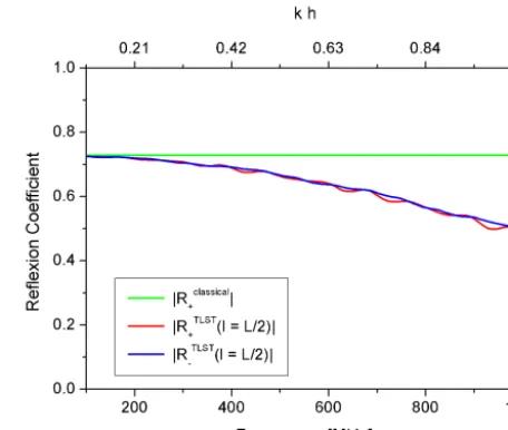
Figure 11. Reflection coefficients|R+e |,|R−e |at the center point for
the classical TL with risers of Fig. 1
e
C+(l)e−j klRe−e−j k(L−l) would travel back. This reflected wave would be reflected again at the beginning of the TL and the current wave i3(l)=Ce+(l)e−j klRe−e−j k(L−l)Re+e−j kl would travel also again to the end of the TL. Theoretically this procedure would be repeated endlessly leading to an ex-pression for the current wave with two infinite sums
i(l)=eC+(l) ∞ X
n=0
e−j kLRe−e−j kLRe+ n
e−j kl
+C+(l)ee −j kLR−e
∞
X
n=0
e−j kLR+ee −j kLR−e n
e−j k(L−l).. (27)
The two sums in Eq. (27) represent geometrical series and can be simplified leading to the final result for the current on the TL
i(l)=Ce+(l) e
−j kl+ e
R−e−2j kLej kl
1−Re−Re+e−2j kL
. (28)
It has to be mentioned that for the asymptotic region, that is
l∈ [L1, L2], the reflection coefficients are constant.
When the current on the TL is known for example from a full wave simulation the current reflection coefficients can be calculated. This is shown forRe+(l). For the asymptotic region a backward traveling wave can be expressed asi(l)=
e
I1 ej kl+Re+e−j kl
. A straight forward calculation results in
e
R+(l)=
j ki(l)−di(l)
dl
j ki(l)+di(l)
dl !
e2j kl. (29)
Figure 12. Current for different positions on the TL calculated us-ing the reflection coefficients.
r0=0.5 mm. The TL is driven by a voltage sourceU0=1 V with source impedanceZ0=50and terminated by a load
ZL=50. Elements of the parameter matrix P ∗(1)
(TLST) are shown in Figs. 2 and 3. Using formulas Eqs. (19) and (18) the current reflection coefficients|Re+|and|Re−|were calcu-lated for the center position on the TL atl=L/2 in the fre-quency range from 100 MHz to 1 GHz as shown in Fig. 11. It is clearly seen that the current reflection coefficients deviate from their classical value significantly with rising frequency because of the radiated energy losses. Because source and load impedance are the same in this configuration,|Re+|and
|Re−|have the same value.
Using Eq. (28) the current can be calculated for different positions and frequencies. Fig. 12 shows the results for the positions L1,L/2 andL2. Also shown (black dash-dotted line) is the current |I (L/2)| resulting from a MoM calcu-lation using the Concept-II code (Brüns et al., 2011). The correspondence between full wave analysis and calculation using novel local and frequency dependent reflection coeffi-cients is excellent.
In Fig. 13 the reflection coefficients|Re−|are shown for the TL from Fig. 1 withh=5 cm for different loadsZL (short circuited, 50, matched and open). The source impedance remains atZ0=50, so|Re+|is the same for allZLvalues and is explicitly shown for the open case. The classical cur-rent reflection coefficient for an open TL is negative because of the necessary phase shift of the current wave. In Fig. 13 the absolute value ofRe−is presented, but of course forω→0 the real part ofRe−would tend to the value−1. For a matched load the classical reflection coefficient is zero. That means the current wave would completely be absorbed in the load and no reflected wave would be produced. In a real TL with risers there is no fixed matched load for all frequencies any longer (Rambousky et al., 2013b). The nonuniformity of a
Figure 13. Reflection coefficients at l=L/2 for different load impedancesZL.
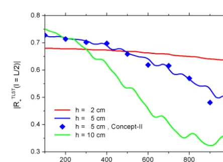
Figure 14. Reflection coefficients atl=L/2 for different heightsh
of the TL over PEC ground.
real TL is responsible for the scattering of the current wave at the local (e.g. bends) or distributed (e.g. varying height over ground) scattering centers. With a classical matched load impedance the current reflection coefficient|Re−| rises with frequency as can clearly be seen in Fig. 13.
Another interesting fact is the influence of the height h
of the TL over ground on the reflection coefficient. With de-creasing heightha TL should show increasingly classical be-havior. This can be seen also in the gradient of the reflection coefficients. In Fig. 14 it is shown that for decreasing heighth
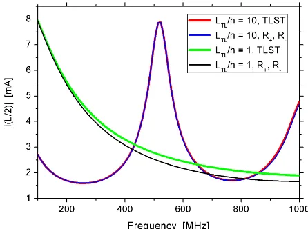
Figure 15. Current at the middle of the TL (l=L/2) for a constant heighth=5 cm and different horizontal lengthLTL.
As mentioned before the original TLST calculation of the current on the TL is an exact solution while the calcu-lation using the novel reflection coefficients is still an ap-proximation because the mutual influence of the risers is neglected. When the ratio of the horizontal part of the TL and the height above the conducting ground plane,LTL/ h, is large enough there will be no significant influence due to the risers. The current on the TL then should be the same as for a pure TLST calculation and a current calcu-lation using the above reflection coefficient method at least for the asymptotic region. This can be seen in Fig. 15 for the ratioLTL/ h=50 cm/5 cm=10. The correspondence is nearly perfect. Reducing the ratio dramatically toLTL/ h= 5 cm/5 cm=1 where the length of the horizontal part is equal to the height of the risers, there is a distinct mismatch between the two current calculation procedures (see also Fig. 15). But from a practical point of view the differences are not crucial so that for practical applications the reflection coefficient method can be used even with smallerLTL/ h ra-tios.
6 Conclusion
In this paper it was shown that cTLT is not sufficient for a fi-nite classical TL with risers at high frequencies. For efficient analysis the TL can be separated into the two riser parts and the asymptotic region. The latter can be handled with cTLT while the riser parts have to be calculated using an advanced TLT, like TLST. The product of matrizants for the three parts finally gives the matrizant for the original whole TL.
Novel reflection coefficients were defined according to the concept of the constant classical ones which are now local and frequency dependent. The current on the TL was calcu-lated using these novel reflection coefficients. For TLs where the horizontal part is significantly larger than the height of the risers the so calculated current fits very well to the
ex-(SEM) analysis of the basic frequencies of a TL system. The extension of SEM for nonuniform TL will be of interest for future work.
Edited by: F. Gronwald
Reviewed by: two anonymous referees
References
Brüns, H., Freiberg, A., and Singer, H.: CONCEPT-II Manual of the Program System, user manual, Technische Universität Hamburg-Harburg, 2011.
Gantmacher, F.: The theory of matrices, Chelsea Publishing Com-pany, New York, 1984.
Haase, H.: Full-Wave Interactions of Nonuniform Transmission Lines, in: Res Electricae Magdeburgenses (MAFO Vol.9), edited by: Nitsch, J. and Styczynski, Z., Magdeburg, 2005.
Haase, H. and Nitsch, J.: Full-wave transmission-line theory (FWTLT) for the analysis of three dimensional wire-like struc-tures, in: Proc. 14th International Zurich Symposium and Tech-nical Exhibition on Electromagnetic Compatibility, 235–240, Zurich, Switzerland, 2001.
Haase, H., Nitsch, J., and Steinmetz, T.: Transmission-Line Super Theory: A New Approach to an Effective Calculation of Electro-magnetic Interactions, The Radio Science Bulletin, 307, 33–60, 2003.
Nitsch, J. and Tkachenko, S.: High-Frequency Multiconductor Transmission-Line Theory, Found. Phys., 40, 1231–1252, 2010. Nitsch, J., Gronwald, F., and Wollenberg, G.: Radiating Nonuni-form Transmission-Line Systems and the Partial Element Equiv-alent Circuit Method, Wiley, Chichester, West Sussex, UK, 2009. Rambousky, R., Nitsch, J., and Garbe, H.: Analyzing Simplified Open TEM-Waveguides using Transmission-Line Super Theory, in: International Symposium on Electromagnetic Compatibility, EMC EUROPE 2012, 1–6, Rome, Italy, 2012.
Rambousky, R., Nitsch, J., and Garbe, H.: Application of the Transmission-Line Super Theory to Multiwire TEM-Waveguide Structures, IEEE Trans. EMC, 55, 1311–1319, 2013a.