Simulation of steady state models describing hybrid desalination process using MATLAB software

(1)

Discipline of Engineering and Energy

ENG470: Engineering Honours Thesis

Simulation of Steady State Models Describing Hybrid

Desalination Process Using MATLAB Software

A thesis submitted to Discipline of Engineering and Energy, Murdoch University, to

fulfil the requirements for the degree of:

H1264: Bachelor of Engineering Honours [BE (Hons)]

1. Instrumentation And Control Engineering (Honours) (Major) (Primary)

2. Renewable Energy Engineering (Honours) (Major)

5

th

July 2019

Written By: Abdullaziz Al-Farqani

Academic Supervisor: Prof. Parisa A. Bahri

(2)

(3)

Author’s Declaration

I, Abdullaziz Al-Farqani, declare that I am a current student of Murdoch University. The thesis entitled “Simulation of Steady State Models Describing Hybrid Desalination Process Using MATLAB Software” has been prepared for my Semester 1, 2019.

ENG470: Engineering Honours Thesis.

I declare that the report is prepared for my academic requirements. The work prepared is authentic and was undertaken by me during my enrolment for this unit at Murdoch University.

(Electronically Submitted, No Signature Required)

_________________________________________ Abdullaziz Al-Farqani

Student,

(4)

(5)

iii

Abstract

Mathematical model development for hybrid multi-stage flash (MSF) and reverse osmosis (RO) desalination plants has gained attention among researchers. The hybrid MSF-RO plant has been a promising and upcoming technology in the desalination market due to its efficient and cost-effective operation. The hybrid plant shares common intake and the final product of the MSF and RO plants are mixed. The plant model plays a significant role in understanding and analysing the plant performance. In this thesis, a steady state mathematical model for hybrid MSF-RO desalination plant was developed to ensure the accuracy and reliability of the plant model. The developed model was based on material, salt and energy balance. Thermal and physical properties of the brine, distillate, and steam are considered. These properties are calculated as a function of temperature and concentration. In addition, the performance ratio of the MSF plant is determined by increasing the number of the MSF stages. The developed model incorporates nonlinear equations which are solved using fsolve, a nonlinear system solver, in MATLAB software. The number of the MSF stages considered was six stages. Whereas, a single stage RO plant was treated.

(6)

iv

Acknowledgments

This thesis would not have been possible without the following support, advice and encouragement throughout the process of developing this thesis.

First and foremost, my sincere appreciation goes to my academic supervisor, Professor Parisa A. Bahri, Head of Discipline Engineering and Energy, Murdoch University, for your patience, guidance and support as well as imparting your immensurable knowledge to me in this field. You have made this an educational and exciting unit. Your mentorship and invaluable advice as well as feedback have steered me to improve my analytical, creative, technical and thinking skills. Besides the fundamentals of chemical engineering, I have also learnt research integrity through this unit.

A special thanks to my family, especially my father and mother. Your prayers and words of encouragement have been a constant source of support throughout my life. I would also like to thank my wife for all your love, prayers and understanding of my goals and aspiration. Thank you for your patience, support and sacrifice especially as I prepare for this thesis. Thank you for being my inspiration. To my son, thank you for always cheering me up and giving me happiness.

I would also like to express my gratitude to the company (Petroleum Development Oman) I work for in Oman, for the financial support and for providing me the opportunity to study in Murdoch University, Perth, Australia.

(7)

(8)

vii

List of Figures

Figure 1: Process Configuration of the Hybrid MSF-RO System ... 21

Figure 2: Reverse Osmosis System... 22

Figure 3: A schematic diagram of Multi-stage flash with brine recycle... 24

Figure 4: Flashing chamber ... 25

Figure 5: A schematic diagram of the hybrid MSF-RO plant ... 25

Figure 6: Mass balance for stage 1 ... 33

Figure 7: Mass balance for any stage, except stage 1 ... 33

Figure 8: A schematic diagram of the hybrid MSF-RO plant ... 40

Figure 9: Temperature of cooling brine ... 61

Figure 10: Flashing brine temperature ... 62

Figure 11: Distillate temperature ... 62

Figure 12: Vapor temperature ... 63

Figure 13: Concentration of the flashing brine ... 64

Figure 14: Flowrate of the flashing brine ... 64

Figure 15: Distillate flowrate ... 65

Figure 16: Performance ratio of the MSF plant ... 65

Figure 17: Overall heat transfer coefficient ... 66

Figure 18: Log mean temperature difference... 66

Figure 19: Specific heat capacity of the brine and distillate ... 67

Figure 20: Specific heat capacity of the cooling brine ... 67

Figure 21: Boiling point elevation and non-equilibrium allowance ... 68

(11)

x

List of Tables

Table 1: Characteristics of the Spiral Wound Membrane ... 32

Table 2: Simulation Results for a Reverse Osmosis System ... 41

Table 3: Simulation Results of the Temperature(s) and Flowrate(s) Profile of the MSF Process ... 43

Table 4: Temperatures and Flowrates of the Brine Heater, Mixer, and Blowdown ... 46

Table 5: Results for Thermo-dynamic Losses and Thermo-physical Properties ... 48

(12)

(13)

1

Chapter 1: Introduction and Objectives

1.1 Introduction

Potable water depletion has led to the rise of desalination plants to ensure an adequate supply of usable and drinkable water for human needs all around the world. Shortage of rain water and population growth are among the reasons for water depletion (Gude 2018). Freshwater can be obtained by a process of separating undesired solid substances, salts, and minerals, from the raw water; this process is known as desalination (Bazargan 2018). Over three decades, the development indicator of desalination plants has shown exponential growth throughout the world (Arafat 2017). Moreover, during the 20th_{century, performance} indicators of the water-desalting plants proved to be the most feasible globally (El-Dessouky and Ettouney 2002). In terms of plant capacity, large-scale commercial plants were producing nearly 8000 𝑚3/𝑑𝑎𝑦 in the mid-1960s, while the capacity had increased to more than

70 million 𝑚3/𝑑𝑎𝑦 in the early 1970s (Lior 2012). In recent times, there have been huge efforts in the improvement of the desalination plants. Production of fresh water goes beyond 80 million 𝑚3/𝑑ay, and over the last 3 years, it was estimated to go above 120 million 𝑚3/

𝑑𝑎𝑦. Recently, studies have pointed out that sustainable production of water can be obtained by higher flux hydrophobic membranes using renewable energies (Wali 2014). People are now turning to desalination technologies due to their reliability in terms of cost-saving and sustainable environment. Overall, desalination technologies need constant improvement to fulfil future extensive applications (Wang et al. 2011).

(14)

2

energy to operate (Thimmaraju et al. 2018). However, MSF and RO plants are found to be the prominent leading technologies in the desalination market (Kesieme et al. 2013). MSF desalination process, a thermal based plant, has accounted for the largest sector of the desalination market making it the leading source of freshwater (Ali and Kairouani 2016). Some of the MSF advantages include simple and easy to function plants, the flow moves from one stage to another without having moving parts such as pumps, and provides high level of water purification (Thimmaraju et al. 2018). The efficiency of the system can also be improved by adding more stages to increase water product capacity. Another factor that can be considered is the performance ratio which determines the efficiency of the MSF plant. The disadvantages on the other hand, includes high energy consumption which yield to higher capital cost (Thimmaraju et al. 2018).

RO desalination process, membrane-based process, is another promising and widespread technology as it is the least energy consuming process and has higher permeate flux (Camacho et al. 2013). It is known to be mainly available in the coastal regions globally. As there are limited natural hydrological resources, constant research and development (R&D) emphasise on energy consumption reduction (Peñate and García-Rodríguez 2012). The RO technology is a pressure driven membrane process. The advantages of the RO system include low energy requirements, low operating temperature, and low water production cost. While, the disadvantages include sensitivity to quality of feed water, more susceptible to fouling and operating conditions of the plant (Oh, Hwang and Lee 2009).

(15)

3 hybrid MSF-RO process. Such hybridisation results in lower energy requirement of the RO system and high desalting performance of the MSF process (Al-Mutaz 2005).

Among the benefits of hybridising RO process with MSF process include cost reduction on post-treatment process and better water quality as the RO permeate concentration is mixed with the distillate produced from the MSF system (Ericsson and Hallmans 1985). Consequently, this results in lower product concentration compared to a stand-alone RO system. Hence, hybridising RO process with the MSF process is found to be an economical and promising technology. There are only few studies that have focused on the improvement of the hybrid MSF-RO operation.

1.3 Objectives of the Thesis

The current research focuses on four key objectives. First, to develop a mathematical model for the hybrid MSF-RO system. Then, to ensure that the developed model is sufficiently accurate. Third, to compare the correlation and dependence between the hybrid system and stand-alone systems for both MSF and RO will be performed. Finally, the performance for the hybrid system will be evaluated by investigating the findings of the hybrid system through the increase number of stage and the comparison with various researches.

1.4 Significance of the Thesis

(16)

4 of the hybrid MSF- RO system. This will in turn lead to reliability and cost-effective measures.

1.5 Structure of the Thesis

The thesis report is structured into seven chapters demonstrated below:

Chapter 1: Introduction and Objectives

This chapter introduces desalination technologies and some of the key advantages and disadvantages. The topic also discusses different researchers’ works, the objectives of the thesis and the significance of the thesis.

Chapter 2: Literature Review

This chapter shares the meaning of mathematical model in chemical engineering, the plant modelling as well as the benefits of plant modelling. The section also covers researchers’ contribution towards the hybrid system.

Chapter 3: Process Description of the Hybrid MSF-RO System

This chapter introduces the process description of the hybrid MSF-RO system. This section also describes individually the MSF and RO processes.

Chapter 4: Steady State Models of the Hybrid MSF- RO System

(17)

5 Chapter 5: Results and Discussion

This chapter mainly discusses and analyses the simulation results of the hybrid MSF-RO process. This section evaluates the simulation results with various researchers. The results and discussion represent the core of the developed model. In addition, the limitations of the current thesis are also shared in this section.

Chapter 6: Conclusion and Future Work

(18)

6

Nomenclature and Symbols

1

Nomenclature for MSF

𝐴𝑏ℎ Total heat transfer area of brine heater

𝐴𝑟𝑗 Total heat transfer area of stage j

𝐴𝑇 Total heat transfer area

𝐵𝐷 Flow rate of brine blow down

𝐵𝑗 Flow rate of flashing brine leaving stage j

𝐵(𝑗 − 1) Flow rate of flashing brine entering stage j

𝐵𝑁 Flow rate of flashing brine leaving last stage

𝐵𝑂 Flow rate of flashing brine entering first stage

𝐵𝑃𝐸𝑗 Boiling point elevation

𝐶 Concentration (Mass fraction)

𝐶𝐵𝑗 Salt concentration of flashing brine leaving stage j

𝐶𝐵(𝑗 − 1) Salt concentration of flashing brine entering stage j

𝐶𝐵𝑁 Salt concentration of flashing brine leaving last stage

𝐶𝐵𝑂 Salt concentration of flashing brine entering first stage

𝐶𝐹 Salt concentration of feed

𝐶𝑅 Salt concentration of recycle brine

𝐶𝑊 Flow rate of reject seawater

𝐷 Flow rate of distillate

𝐷𝑖_𝐻 _{Internal diameter of brine heater tubes}

𝐷°𝐻 External diameter of brine heater tubes

𝐷𝑖_𝑗 _{Internal diameter of tubes at stage j}

(19)

7

𝐷°𝑗 External diameter of tubes at stage j

𝐷𝑗 Flow rate of distillate leaving stage j

𝐷(𝑗 − 1) Flow rate of distillate entering stage j

𝑓𝐻 Brine heater fouling factor

𝑓𝑗 Fouling factor at stage j

𝐹𝑚 Flow rate of makeup seawater

𝐹𝑠𝑒𝑎 Flow rate of feed seawater

𝐻𝑗 Height of brine pool at stage j

ℎ𝑗 Specific enthalpy of flashing brine leaving stage j

ℎ(𝑗 − 1) Specific enthalpy of flashing brine entering stage j

ℎ𝑚 Specific enthalpy of makeup stream

ℎ𝑅 Specific enthalpy of recycle stream

ℎ𝑤 Specific enthalpy of cooling brine entering heat recovery section

ℎ𝑣𝑗 Specific enthalpy of flashing vapour at stage j

(𝐿𝑀𝑇𝐷)𝑏ℎ Log mean temperature difference for brine heater

(𝐿𝑀𝑇𝐷)𝑗 Log mean temperature difference for stage j

𝑁𝐸𝐴𝑗 Non-equilibrium allowance in temperature for flashing brine for stage j

𝑅 Flow rate of recycle brine

𝑆𝑏ℎ Specific heat capacity of brine in brine heater

𝑆𝐵𝑗 Specific heat capacity of flashing brine leaving stage j

𝑆𝐵(𝑗 − 1) Specific heat capacity of flashing brine entering stage j

𝑆𝐷𝑗 Specific heat capacity of distillate leaving stage j

𝑆𝐷(𝑗 − 1) Specific heat capacity of distillate entering stage j

𝑆𝑟𝑐𝑗 Specific heat capacity of cooling brine leaving stage j

(20)

8

𝑇𝐵𝑗 Temperature of flashing brine leaving stage j

𝑇𝐵(𝑗 − 1) Temperature of flashing brine entering stage j

𝑇𝐵𝑂 Temperature of flashing brine leaving brine heater

𝑇𝐷𝑗 Temperature of distillate leaving stage j

𝑇𝐷(𝑗 − 1) Temperature of distillate entering stage j

𝑇𝐹1 Temperature of cooling brine leaving stage 1

𝑇𝐹𝑗 Temperature of cooling brine leaving stage j

𝑇𝐹(𝑗 + 1) Temperature of cooling brine entering stage j

𝑇𝑟𝑒𝑓 Reference temperature

𝑇𝑠𝑗 Temperature of flashed vapour at stage j

𝑇𝑠𝑡𝑒𝑎𝑚 Steam temperature

𝑈𝑏ℎ Overall heat transfer coefficient at the brine heater

𝑈𝑗 Overall heat transfer coefficient at the brine heater at stage j

𝑊 Flow rate of cooling brine in heat recovery section

𝑤𝑗 Width of stage j

𝑊𝑠 Flow rate of steam

Symbols for MSF

λs Latent heat of vaporisation of water in brine heater

∆𝑗 Temperature drop in demister in stage j

𝜌𝑏 Brine density

𝜌𝑤 Pure water density

Nomenclature for RO

𝐴𝑚𝑒𝑚 Area of membrane

𝐴𝑠 Salt permeability constant

(21)

9

𝐶 Concentration

𝐶𝑏 Bulk concentration

𝐶𝑓 Feed concentration

𝐶𝑚𝑒𝑚 Membrane cost

𝐶𝑝 Permeate concentration

𝐶𝑝𝑣 Pressure vessel cost

𝐶𝑟 Reject concentration

𝐶𝑤 Wall concentration

𝑑 Diameter of element

𝑑𝑓 Feed spacer thickness

𝐷𝑠 Solute diffusivity

𝑓𝑐 Plant load factor

ℎ𝑠𝑝 Height of spacer channel

𝐽𝑠 Salt flux

𝐽𝑤 Water flux

𝑘 Mass transfer coefficient

𝐿𝑚 Length of membrane element

𝐿𝑝𝑣 Length of pressure vessel

𝑚 Number of membrane element in a pressure vessel

𝑁1 Number of leaves in a membrane element

𝑁𝑝𝑣 Number of pressure vessels

𝑃𝑓 Feed pressure

𝑃𝑝 Permeate pressure

𝑃𝑟 Reject pressure

(22)

10

𝑄𝑓 Feed flow rate

𝑄𝑝 Permeate flow rate

𝑄𝑟 Reject flow rate

𝑅𝑒 Reynolds number

𝑆𝑐 Schmidt number

𝑆𝑅 Salt rejection

𝑇 Temperature

𝑤 Membrane width

𝑉 Average axial velocity in the feed channel

Symbols for RO

μ Brine viscosity

𝜋 Osmotic pressure

𝜋𝑓 Osmotic pressure of feed

𝜋𝑝 Osmotic pressure of permeate

𝜋𝑟 Osmotic pressure of reject

∆𝜋 Osmotic pressure drop

∆𝑃 Pressure drop

∆𝑃𝑓 Pressure drop on the feed side

𝜀 Feed spacer void fraction

𝜌 Brine density

𝜌𝑤 Pure water density

Nomenclature for Hybrid MSF-RO

(23)

11

Chapter 2: Literature Review

2.3 Research Background

Several researches have been performed to develop a model for the hybrid MSF-RO process. The following researchers have contributed to the research of each section in one way or another.

2.3.1 Reverse Osmosis (RO) Plant

Al-Mutaz and Al Ghunaimi (2001) researched on performance of RO process at high temperatures. The study went through intensive trials by considering RO characteristics and analysis made theoretically. The study determined that a high-water temperature produces better RO operation by increasing the feed temperature by three percent with the increase in membrane capacity. The study compared data with actual data plant figures.

Oh et al. (2009) studied the RO system for seawater desalination and came up with a simple model based on the theoretical solution-diffusion and multiple fouling mechanism for analysis of the performance of the RO system. The model designed also prove that temperature influences optimisation of sea water reverse osmosis (SWRO) system. The main aim of the develop model is to have a computer model for simulating and optimising the process flow regardless of the types of membranes used. The findings can be further analysed for optimisation purpose.

2.3.2 Multistage Flash (MSF) Plant

(24)

12 total distillate flow rate, reduction of thermic energy consumption as well as minimise sum of flow rates of plant’s main pumps. The authors applied MATLAB software, using response surface methodology (RSM) in this research and the results were based on actual plant data. The outcome of the research led to a set of Pareto2_{optimal solutions. This achieved optimal} plant operation throughout the year.

Husain (2012) developed two approaches to the dynamic models. One approach was to apply the basic dynamic phenomena known as the phenomenological models (used for understanding the process behaviour) and the other was a black-box approach (a simple statistical model used for control purpose). One of the model limitations was its differential energy balance consideration of the combination of vapour space and distillate in the flash stage. The results obtained were tested through experimental or operating data of the process (Husain 2012).

Rosso et al. (1997) found that mathematical models provided an insightful tool which described a steady-state model developed to analyse the MSF desalination process based on detailed physicochemical representation of the process. Essential basic phenomena and geometry of the stages are among features taken into consideration. The authors’ studies were further supported by El-Dessouky, Shaban and Al-Ramadan (1995), Ali and Kairouani (2016), as well as, Alasfour and Abdulrahim (2008). These authors supported the steady-state mathematical model built with the intention to analyse the efficiency of the MSF performance. The model took into account the relationships between parameters controlling the water cost to other operating and design variables established (El-Dessouky, Shaban and Al-Ramadan 1995). This included models which applied investigation to effects of varying

2 _{Pareto optimality is defined as an analytical tool which is utilised to assess social welfare and}

(25)

13 cooling water temperatures and/or flow rates on plant performance at constant distillate production and steam consumption (Alasfour and Abdulrahim 2009).

2.3.3 Hybrid MSF-RO Plant

Gambier and Badreddin (2003) focused on recent efforts in control theory. The authors’ efforts took into considerations not only intrinsic hybrid processes, but also continuous processes with supervisory logic, multi-model control systems and switching control. Introduction to the hybrid modelling and control pathed the way to development of design tools and difficult computer controlled systems.

Talati (1994) discussed about RO and evaporation (MSF and MED) in treating desalination. The author concentrated on the expected cost when different feedwater sources were used by RO and MSF/MED to produce high-purity water and identified three processes in the course of research. The results revealed that the RO process was the most cost effective, which met the feedwater requirements as well as reject water generation (Talati 1994).

(26)

14 Helal et al. (2003) on the other hand, took into consideration hybrid MSF-RO configurations and utilised the Newton-Raphsons3 using SOLVER Tool of Microsoft Excel. Helal et al. (2003) considered some operating variables such as steam temperature, cooling seawater flow rate, make up flow rate and brine recycle flowrate in their studies. One unique feature of this study was that the reject flowrate was fed into the RO process. In the current thesis, the reject flowrate is sent back to the sea.

The hybrid system model designed incorporates nonlinear models which are accurate based on results obtained from different researchers. No comprehensive studies have since been carried out thus far; only semi-empirical equations calculations based on semi-empirical equations have been reported (Al-Shayji, Al-Wadyei and Elkamel 2005).

In this thesis, a steady state mathematical model of the hybrid MSF-RO process was developed to enhance the operation of the hybrid system and further improve the process model efficiency.

2.4 Researchers’ Contribution towards the Hybrid System

As mentioned in chapter one, many researchers have performed researches on stand-alone MSF and RO processes. Studies have also revealed that researchers are interested in both dynamic and steady-state hybrid MSF-RO model. Although there has been an increase in interest in analysing the cost and benefits of the stand-alone MSF and RO models, there are still limited studies in improvement of the hybrid MSF-RO operation. Giving strong

3 _{Newton-Raphson method is a system of equations, useful for discovering quick roots of nonlinear}

(27)

15 consideration to the advantages of both MSF and RO, the hybrid MSF-RO is found to be a promising technology in terms of cost reduction and final product quality. Importance should not be confined to optimisation, instead control design should be given equal attention to ascertain its importance when designing a hybrid MSF-RO model. The lack of research findings in the hybrid systems inspires the need for enhancing the operation of the hybrid system in the most efficient and cost-effective manner.

The following researchers have contributed significantly to the hybrid system. Their works have been observed and summarised in this topic.

Elmesmary and Alsultan (2017) carried out a study on hybridisation of the MSF and RO processes with the aim to improve the effectiveness of the final product as well as to maximise the recovery ratio and quality of the process for cost reduction purpose. The study emphasised more on research for the hybrid system model by describing various models rather than using a specific software for analysing and evaluating the results. The study concluded by sharing the authors’ opinions on the required studies for hybrid systems improvement as MSF- Multi-Effect Distillation (MED) has similar advantages to MSF-RO. The authors mentioned that they had intentionally ignored some of the key processes of desalination to better demonstrate hybridisation of desalination processes. The limitations observed by future researchers to ensure the desired outcome should not affect when comparing their obtained outcomes with these authors study.

(28)

16 up of different cases such as interdependent two-stage RO and brine recycle MSF plants with common intake-outfall facilities, and hybrid single-stage RO/brine recycle MSF plant. The mathematical model applied to brine recycle MSF plant model for the purpose of comparing different alternative schemes and reducing the computation time. In this study a Newton-Raphson method was applied to obtain the minimum value of the objective function using SOLVER tool of Microsoft Excel (Helal et al. 2003). One unique feature of this research was that the reject flowrate leaving the MSF was fed into the RO system.

Similar to Helal et al. (2003), Hamed (2005) focused on a single stage RO process which was coupled with the MSF process. However, Hameed (2005) further reviewed the integrated hybrid desalinations systems by using nanofiltration (NF) membranes to reduce the significant impact of ions from seawater. The author further concluded that the hybrid MSF-RO produced efficiently high-water productivity. Whereas, the make-up of the MSF unit formed from the RO reject blended with appropriate measurements of seawater was successful (Hamed 2005). The author mentioned that further research work will be required for NF. Similarly, Elmesmary and Alsultan (2017) agreed with Hamed (2005) and realised the potential in combining the MSF and MED processes for further development. Nonetheless, Elmesmary and Alsultan (2017) further added that the RO process with nanofiltration pre-treatment should also be researched.

(29)

17 1998). As their study showed corrected product water concentration was similar to feed water temperature, there were still no concrete evidence on whether membrane capability for salt rejection had any correlation to higher operating performance as this was not within the scope of the research. Thus, assumptions provided in this area of study were authors’ opinions.

On the other hand, Al-Mutaz (2005) focused his study on the main strengths of both stand-alone MSF and RO systems (high distilled performance, low energy requirement). The author mentioned that the reject flow from the MSF plant can be applied to optimised feedwater temperature of the RO plant. This high feed temperature was beneficial as the constant pressure obatined from the water flux of the membrane slightly increased the temperature and in turn increased the RO productivity. Unlike El-Sayed et al. (1998), Al-Mutaz (2005) was able to confirm that there were correlation between lower salt rejection and feed water temperature as it increased. The author concluded with the advantages of hybrid MSF and RO, indicating hybrid system could lead to various positive outcomes such as extended membrane life and improved performance, as well as low power and low production cost.

Alasfour & Abdulrahim (2009) focused on designing a rigorous steady state modelling which would simulate the MSF with brine circulation (MSF-BR). The software used was IPSEpro®, to facilitate a meticulous simulation of the processes using the thermo-physical properties models, which were calculated as a function of temperature and salinity. The MSF-BR processes was assessed based on performance prediction of the first and second law of thermodynamics (Alasfour and Abdulrahim 2009). This study provided positive results between the computational and actual plant data. As the results were validated, the authors’ foundation paths way for future works to be carried out more easily.

(30)

18 then used to determine the optimal process design and optimum values for a defined water production. The outcome yielded to the basic design of the hybrid system. However, it was noted that Marcovecchio et al. (2005) used MSF-Once through (MSF-OT) whereas, Alasfour and Abdulrahim (2009) used MSF-Brine recycle (MSF-BR).

Bandi, Uppaluri and Kumar (2016) focused on global optimisation of hybrid MSF-RO desalination processes using differential evolution algorithm. The authors focused on five hybrid process configurations. The first was where MSF-BR and a single stage RO system (SRO) receives seawater directly using fluid delivery pump. The second indicated the cooling water stream was fed as the feed stream to a single reverse osmosis (SRO) system. The third process involved the cooling brine stream leaving the mixer one with flow rate then it splits to three streams - the MSF recycle stream and MSF blow downstream with feed flowrate of reject stream. The fourth hybrid indicated that the cooling water stream fed to the SRO process and the fifth hybrid indicated the schematic process where reject water stream was fed as feed stream to SRO. The sequential quadratic programming (SQP) algorithm in MATLAB optimisation toolbox and its variants were deliberated in this study. The outcome revealed that the fourth hybrid provided lowest freshwater production cost.

(31)

19 Another study which was conducted was by Kumar, Dewal and Mukherjee (2013). The study demonstrated that the authors were aware of the need for seawater desalination and considered the hybridisation of the two prominent technologies of the MSF-BR and RO processes to complement each other. The development of Supervisory Control And Data Acquisition(SCADA), was used to monitor the hybrid MSF-BR and RO process. The control system also considered the MSF seawater (reject cooling seawater to feed RO) to develop and stimulate the process. Human Machine Interface(HMI) navigated the whole process of controling and monitoring. The strenght of the researcher included detailed step by step guide of the operational details. However, the lack of sharing the actual feed flow would make it harder for the future researchers to progress on from this research work.

(32)

(33)

21

Chapter 3: Process Description of the Hybrid MSF-RO System

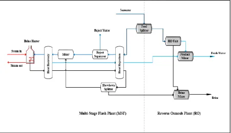
The process configuration of the hybrid MSF-RO process considered in this thesis refers to hybridisation of the MSF-BR process with a single stage RO process (as illustrated in Figure 1). The following sections demonstrate descriptions of the hybrid MSF-RO process.

Figure 1: Process Configuration of the Hybrid MSF-RO System (Malik, Bahri and Vu 2016)

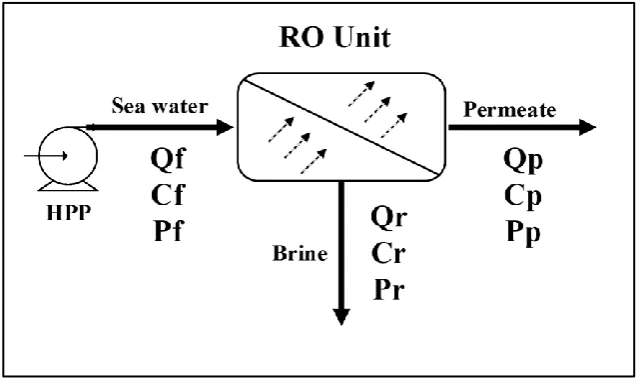
3.1 Reverse Osmosis (RO)

(34)

22 RO membrane cannot achieve 100% salt rejection, the permeate flow contains a small amount of salts residues (Cp). While the undesired brine solution (Qr) with concentration (Cr) is rejected. The RO module (spiral wound) is made up of a set of pressure vessels (hollow tube), which encompass the RO membrane elements. The pressure vessel may contain up to eight membrane elements. The type of the spiral wound element considered in this thesis is a flat sheet, cylindrical cross flow filtration.

An important stage is that, raw feedwater is pre-treated to deflocculate the undesired substances before being pumped into the reverse osmosis module (Bachoo and Sastry 2016). Pre-treatment is a very important step in this desalination plant to reduce membrane degradation rate. At the last stage, the post-treatment step is where additive chemical is added into a storage tank for better quality of freshwater (El-Ghonemy 2017).

(35)

23

3.2 Multi-stage Flash (MSF)

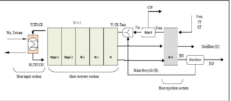
Figure 3 demonstrates MSF with brine recycle (MSF-BR). The MSF plant mainly constitutes of heat input section, heat recovery section and heat rejection section. The heat input section is made up of a brine heater where the temperature of seawater is raised at maximum temperature. The heat recovery and heat rejection sections are divided into a number of stages. In this thesis, the number of heat recovery stages is considered five stages, whereas, only one stage is considered for heat rejection section as illustrated in Figure 3. Additional components such as water reject splitter, blowdown splitter, and mixer are also illustrated.

(36)

24 The cooling brine flows through a series of condensers in each stage to condense the flashed vapour. The temperature of feed seawater (TF) keeps increasing by absorbing the latent heat produced by flashing brine in each stage. The cooling brine stream then enters the heat input section, where it is heated by steam flowrate (Ws) which is fed into the brine heater, at maximum temperature. This temperature is known as top brine temperature (TBT).

The flashing brine flowrate (B0) leaving the brine heater at TBT is directed into the first stage of the heat recovery section. The flashing brine flashes off and produces distillate vapour (As shown in Figure 4). Consequently, the temperature of the flashing brine keeps decreasing as the vapour is continuously flashed in each stage. The flashed vapour flows across the demisters or eliminators to remove the brine droplets. The distillate vapour or the pure vapour is condensed by condenser tubes to form distilled water which is collected in the distillate tray. This process continues all the way down the plant.

(37)

25

Figure 4: Flashing chamber (Ali and Kairouani 2016)

3.3 Hybrid System (MSF-RO)

Figure 5 shows a simplified schematic diagram of the hybrid MSF-RO process shown above in the first section of this chapter. The hybrid system shares common intake and the final product of distillate flowrate (D) produced from MSF process and permeate flowrate (Qp) produced from the RO process is combined. On other hand, the rejected flowrate (Qr) and blowdown flowrate (BD) rejected from the RO and MSF processes, respectively, are mixed and then pumped out of the hybrid process. The cooling seawater flowrate (CW)rejected from the reject separator of the MSF is not utilised in the process.

It can be seen that the final concentration of the RO process (Cp) is mixed with pure distillate produced from the MSF process, which is assumed salt free.

(38)

26

Chapter 4: Steady State Models of the Hybrid MSF-RO System

4.1 A Mathematical Model in Chemical Engineering

In science and technology, mathematical models play an important role in the life of scientist, engineers and researchers. The process of developing, understanding and applying mathematical equations defines mathematical modelling (Rasmuson et al. 2014). The system performance would rely on the firm foundation of a mathematical modelling and simulation tools which includes analytical and numerical techniques for solving mathematical model equations such as nonlinear algebraic equations (Chidambaram 2018). In short, the mathematical model describes equations, function, facts and data using mathematical tools, methods and terminology. Depending on the type of process model required, the mathematical model would differ from one to another. A mathematical model requires precision and unambiguity based on understanding a mutual framework. Steps would include identifying and understanding the parameters, sorting the required data based on relevancy, seeking for solutions to the issues faced by arranging and analysing the data based on requirements, then to come up with a reasonable conclusion (Marion and Lawson 2015).

4.2 Plant Modelling

(39)

27 significance of the model building is to give the analysts a transparent insight into behaviour of plant which can subsequently be controlled and optimised (Cameron and Hangos 2001).

4.2.1 Benefits of Plant Modelling

Some benefits of plants modelling are demonstrated as follows (Cameron and Hangos 2001):  Investigate the behaviour of the plants against reality.

 Enable the analyst to perform optimization, design, and control of systems.  Enable the analysts to validate data quality and quantity.

 Introduce process parameters estimation  Manage process risks that may take place.

4.3 Methodology

This chapter focuses on the methods to achieve the objectives of this thesis. The steps taken include hypothesis, collecting of data, experiment, and analyse the research objectives. The scientific method which involves a systematic process flow has been applied to this research.

(40)

28 solver. The developed model incorporates a set of nonlinear algebraic equations which will be solved simultaneously.

The accuracy of the developed model will be further evaluated and examined. Any undesired outcomes will warrant a repeat in the process flow from the prediction stage. By iterating to convergence, the predicted value will be tested to ensure its validity through the comparison of works by different researchers.

4.4 List of Assumptions

A list of assumptions is made to simplify the chemical engineering problems. In this thesis, the following assumptions are:

 The flashed vapour is free from brine droplet.

 Temperature profiles of the flashing brine, distillate, and cooling brine are linear.  Distillate produced in each stage is salt-free.

 Thermal and physical properties for the brine, distillate, and seawater are a function of both salinity and temperature.

 Heat of mixing flashing brine is negligible.  In the brine heater, no sub-cooling of condensate.

4.5 Reverse Osmosis Process Model

(41)

29 Mass balance:

Qf = Qp + Qr (1)

Salt balance:

Qf∗CF = Qp∗Cp + Qr∗Cr (2)

The recovery ratio (%):

Qp/Qf ∗ 100 (3)

Average velocity in feed side (𝑚/𝑠):

V = Qb/(w ∗ hsp ∗ ε) (4)

Pressure drop (𝑘𝑃𝑎):

∆P = Pf − ∆Pf/2 − Pp (5)

Pressure drop on the feed side (𝑘𝑃𝑎):

∆Pf = (0.003 ∗ Qb ∗ 3600 ∗ Lpv ∗ μ)/(w ∗ d3₎ ₍₆₎

Osmotic Pressure (𝑘𝑃𝑎):

π = (0.2641 ∗ C ∗ 1000 ∗ (T + 273))/(106_{− (C ∗ 1000))} ₍₇₎

Osmotic pressure difference (𝑘𝑃𝑎):

(42)

30 Water flux (𝐿/𝑚2 𝑠):

Jw = Aw ∗ (∆P − ∆π) ∗ 1000 (9)

Salt flux (𝐿/𝑚2 𝑠):

Js = As ∗ (Cw − Cp) (10)

Average bulk concentration (𝑔/𝐿):

Cb = (Cf + Cr)/2 (11)

Concentration Polarization:

Cw − Cp Cb − Cp = e

Jw

ρ∗k ₍₁₂₎

Mass transfer coefficient (𝑘𝑔/𝑚3 𝑠):

k = 0.04 ∗ Re0.75_{∗ Sc}0.33_{∗ (Ds/df)} ₍₁₃₎

Salt Rejection (%):

SR = 1 −Cp_Cf (14)

Length of the pressure vessel (m):

(43)

31 Membrane width (m):

w = Amem/(Lm ∗ N1) (16)

Reynolds number:

Re = (ρ ∗ df ∗ V)/μ (17)

Schmidt number:

Sc = μ/(ρ ∗ Ds) (18)

In this current study, the brine viscosity (𝜇) and solute diffusivity (𝐷𝑠) are calculated as a function of temperature and salinity:

μ = 1.234𝑥10−06_{∗ exp^(0.00212 ∗ 𝐶 + (1965/(273 + 𝑇)) )} ₍₁₉₎

𝐷𝑠 = 6.725𝑥10−06_{∗ exp^(0.154𝑥10}−03_{∗ 𝐶 + (2513/(273 + 𝑇)) )}

(20) The unit of:

Brine viscosity is 𝑘𝑔/𝑚 𝑠 Diffusivity coefficient is 𝑚2/𝑠

However, the average brine density (kg/m3) is considered as a constant value of 1020 𝑘𝑔/

(44)

32

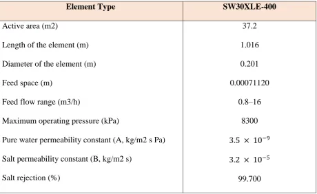
Table 1: Characteristics of the Spiral Wound Membrane

Element Type SW30XLE-400

Active area (m2)

Length of the element (m) Diameter of the element (m) Feed space (m)

Feed flow range (m3/h)

Maximum operating pressure (kPa)

Pure water permeability constant (A, kg/m2 s Pa) Salt permeability constant (B, kg/m2 s)

Salt rejection (%)

37.2 1.016 0.201 0.00071120 0.8–16 8300

3.5 × 10−9

3.2 × 10−5 99.700

4.6 Multi-stage Flash Process model

The developed model of the MSF is taken from Malik, Bahri and Vu (2016), Rosso et al. (1996), and Abdul-Wahab et al. (2012). The following sub-sections demonstrate the mass, salt, and energy balance equations. In addition, thermo-dynamic losses and thermo-physical properties of the brine and steam are presented. The specific heat capacity of the flashing brine, distillate, and cooling brine are shown.

5.3.1 Mass balance equations for each stage

(45)

33

B_j₋₁+ D_j₋₁ = B_j+ D_j (21) Mass balance for stage 1:

B₀ = B₁+ D₁ (22)

Note that there is no distillate flow rate entering the first stage (D0 = 0). As illustrated in Figure. 6

Figure 6: Mass balance for stage 1 (Abdul-Wahab, et al. 2012)

(46)

34

5.3.2 Salt balance equation for each stage

Component balance (salt) for any stage in both heat recovery or heat rejection sections is given as:

B_j₋₁. C_Bj−1= B_j. C_Bj ₍₂₃₎

Note that the cooling brine flowrate (W) and the concentration of the cooling brine (CR) do not change at any stage of the heat recovery section. This applies also to the cooling brine flowrate (Fsea) and the feed concentration (CF) in the heat rejection section.

5.3.3 Enthalpy balance of the heat recovery and heat rejection sections

The overall enthalpy balance for any stage of heat recovery section is given as:

W. Srcj. (TFj− TFj+1)

= D_j−1. SD_j−1. (TD_j−1− Tref) + B_j−1. SB_j−1. (TB_j−1− Tref)

−Dj. SDj. (TDj− Tref) − Bj. SBj. (TBj− Tref) (24)

The specific heat capacity of the cooling brine (Srcj) is calculated as a function of temperature (TFj) and concentration (CR):

Srcj = 4.185 − 5.381x10−03_{∗ CR + 6.26x10}−06_{∗ CR}2_{− (3.055x10}−05

+ 2.774x10−06_{∗ CR − 4.318x10}−08_{∗ CR}2_{) ∗ TFj}

+ (8.844x10−07_{+ 6.527x10}−10_{∗ CR − 4.003x10}−10_{∗ CR}2₎

∗ TFj2 (25)

(47)

35 The specific heat of flashing brine (SBj) is calculated as a function of temperature (TBj) and concentration (CBj):

SBj = (1 − Cbj ∗ (0.011311 − 1.146e − 05 ∗ TBj)) ∗ SDj ₍₂₆₎

The specific heat capacity of distillate (SDj) is calculated as a function of temperature (TDj) and concentration (CB):

SDj = (1.0011833 − 6.1666652e−05_{∗ TBj + 1.3999989x10}−07_{∗ TBj}2₊

1.3333336x10−09_{∗ TBj}3₎(27)

Enthalpy balance of the flashing brine for any stage is given as:

Bj−1. hj−1= Bj. hj+ (Bj−1− Bj). hvj (28)

Where:

hj and hvj are calculated by the following formula:

ℎ𝑗 = (4.186 − 5.381𝑥10−3_{∗ 𝐶𝐵𝑗 + 6.26𝑥10}−6_{∗ 𝐶𝐵𝑗}2_{) ∗ 𝑇𝐵𝑗}

− (3.055𝑥10−5_{+ 2.774𝑥10}−6_{∗ 𝐶𝐵𝑗 − 4.318𝑥10}−8_{∗ 𝐶𝐵𝑗}2₎

∗ 𝑇𝐵𝑗2

+ (8.844𝑥10−7_{+ 6.527𝑥10}−8_{∗ 𝐶𝐵𝑗 − 4.003𝑥10}−10_{∗ 𝐶𝐵𝑗}2₎

∗ 𝑇𝐵𝑗3

(29)

hVj = 596.912 + 0.46694 ∗ TDj − 0.000460256 ∗ TDj2 (30) The distillate temperature (TDj) can be calculate by the equilibrium equations:

TDj = TBj – (BPEj + NEAj + ∆j ) (31) Where:

The Boiling point elevation (BPE) is calculated by:

BPEj = Cj ∗ TBj/(266919.6 − 379.669 ∗ TBj + 0.334169 ∗ TBj2_{) ∗}

(565.757/TBj − 9.81559 + 1.54739 ∗ log(TBj) − Cj ∗ (337.178/TBj − 6.41981 + 0.922753 ∗ log(TBj) + Cj2_{∗ (32.681/TBj − 0.55368 +}

0.079022 ∗ log(TBj))))

(48)

36 Where:

C =19.819 ∗ Cb

1 − Cb (33)

𝐶𝑏 = Salt Concentration (fraction)

The non-equilibrium allowance (NEA) is calculated by:

NEAj = (195.556 ∗ H_rc1.1_{∗ (}omgrc

1000)

0.5

)/(dTBj0.25_{∗ Tsj}2.5₎ ₍₃₄₎

The temperature drop in demister (∆) is calculated by:

∆𝑗 = exp(1.885 − 0.02063 ∗ 𝑇𝐷𝑗) (35)

BPEj, NEAj, and ∆j are the thermodynamic losses.

Distillate and flashed steam temperature correlation is given as:

Tsj = TDj + ∆j (36)

Heat transfer model at the condenser for heat rejection section:

Fsea ∗ Srcj ∗ (TFj – TF(j + 1)) = Uj ∗ Aj ∗ (LMTD)j (37)

Where:

Uj (overall heat transfer coefficient) is now calculated as a function of (Fsea, TFj, TFj +

1, TDj, Dji_{, Dj}o_{, fj}_{) and taken from Helal et al. (2003):}

Uj = 1.0/(Yj + Zj) (38) Where:

(49)

37

Yj = vj ∗ Di(0.2)_{/(160 + 1.92 ∗ vj ∗ TDj)} ₍₃₉₎ vj represents the velocity of the cooling brine flowrate (Fsea) for the heat rejection section and 𝐷𝑖 is the internal diameter of tubes at any stage j.

Zj is defined as the sum of other thermal resistance such as steam-side condensing film, steam-side fouling, tube metal and brine-side fouling. Zj is given by

Zj = 10.24768x10−04_{− 74.73939x10}−07_{TDj + 0.999077x10}−07_TDj2

− 0.430046x10−09_TDj−3_{+ 0.6206744x10}−12_TDj4 (40)

Note: some variables and parameters in the equations will change between heat rejection and heat recovery sections (see Nomenclature and Symbols section).

Heat transfer model at the condenser for heat recovery section:

W ∗ Srcj ∗ (TFj – TF(j + 1)) = Uj ∗ Aj ∗ (LMTD)j (41)

Note that, Uj is defines as equation (40) except that Fsea is replaced by W and inside diameter (𝐷𝑖).

5.3.4 Mixer and splitters equations

Mixer combines both makeup flowrate (Fm) rate and brine recycle flowrate (R) to form cooling brine flowrate (W). The mass and salt balances around the mixer are given as:

Mass balance:

W = R + Fm (42) Salt Balance:

(50)

38 Energy balance:

W ∗ hw = R ∗ hR + Fm ∗ hm (44)

hw, hR, and hm are calculated as a function of (Tr, Cr), where Tr and Cr are the respective stream of both temperature and concentration.

Blowdown splitter separates the flashing brine flowrate (BN) leaving the heat rejection section into brine recycle (R) and blowdown (BD) flowrates.

Mass balance around the blowdown splitter is given as:

BN = BD + R (45)

The concentration of flashing brine entering the blowdown splitter is the same as the concentration leaving the splitter.

On the other hand, in the reject water splitter, feed seawater flowrate (Fsea) enters the splitter and part of the feed seawater flowrate is rejected (CW). The outlet stream leaving the splitter is called makeup flow (Fm). Mass balance around the reject water splitter is given as:

Mass balance:

Fsea = CW + Fm (46)

Similar to the blowdown splitter, the feed concentration of the reject water splitter is the same as the concentration of the makeup flow rate (Fm) and reject flow rate (CW).

5.3.5 Brine Heater enthalpy balance

The energy balance around the brine heater is given as:

(51)

39 Where:

λs = Latent heat of vaporization of water (kJ/kg)

Sbh = Specific heat capacity of brine in brine heater (kJ/kg °C)

TBT = Top Brine Temperature (°C)

𝑇𝐹1 = Temperature of the cooling brine leaving stage 1 (°C)

𝜆𝑠 is calculated as a function of steam temperature (Tsteam):

hV = 596.912 + 0.46694.∗ Tsteam − 0.000460256 ∗ Tsteam2 ₍₄₈₎

hD = 1.8 ∗ (−31.92 + 1.0011833 ∗ (Tbp) − 3.0833326x10−05_{∗ (Tbp)}2

+ 4.666663x10−08_{∗ (Tbp).}3_{+ 3.333334x10}−10_{∗ (Tbp)}4₎ ₍₄₉₎

λs = (hV − hD) (50)

𝑆𝑏ℎ is calculated by a function of TBT and TF1:

Sbh = 1.0011833 − 6.1666652x10−05_{∗ (.}(TF1+TBT)

2 ) + 1.3999989x10 −07_.∗

(.(TF1+TBT)₂ ) .2_{+ 1.3333336x10}−09_{.∗ (.}(TF1+TBT) 2 ) .

3

(51)

Brine heater transfer model:

Ubh ∗ Abh ∗ (LMTD)bh = Ws λs (52)

Where:

Ubh (overall heat transfer coefficient of the brine heater) is calculated as a function of (W, TBT, TF1, TDj, DiH , D°H , fj). Ubh is defined as same equation as Uj is calculated in heat rejection section. Note that Fsea is replaced by W and the temperature and inside diameter of the heat exchanger is different.

(52)

40

LMTD = (TBT – TF1)/log((Tsteam – TF1)/(Tsteam − TBT)) (53)

Brine heater balance: W = B0 (54) Brine heater salt

balance:

CR = CB0

(55)

The overall balance and salt balance of the MSF is given as: Overall balance:

Fm = D + BD (56)

Overall salt _{Fm ∗ CF = BD ∗ CBN}

(57)

4.7 Hybrid System (MSF-RO)

The hybrid system of MSF and RO share common intake and the final product of both systems are mixed. The final concentration (CT) represents the concentration of the final product obtained from the average concentration of both product concentrations of stand-alone MSF and RO. The mass and salt balances are given as:

Mass balance: Final Product = Distillate + Permeate (58) Salt balance: Final Product ∗ CT = Permeate ∗ Cp (59)

𝑪𝒑 𝑪𝑻

(𝑪𝑾)

(𝑩𝑫)

(𝑸𝒓)

(53)

41

Chapter 5: Results and Discussion

5.1 Reverse Osmosis (RO)

Table 2 shows simulation results for a reverse osmosis system. The input data used to solve the process model are taken from both Malik, Bahri and Vu (2016) and Lu et al. (2007). The feed flowrate (𝑄𝑓) and feed concentration (𝐶𝐹) are given as input data. Other process variables have been calculated as illustrated below.

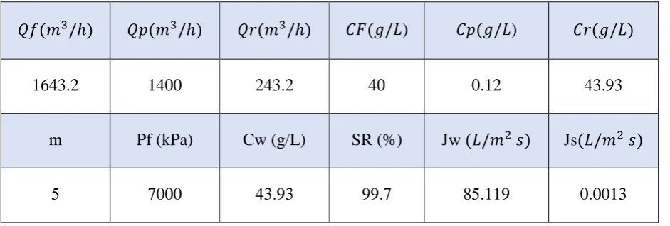
Table 2: Simulation Results for a Reverse Osmosis System

𝑄𝑓(𝑚3_/ℎ) _{𝑄𝑝(𝑚}3_/ℎ) _{𝑄𝑟(𝑚}3_/ℎ) _{𝐶𝐹(𝑔/𝐿}₎ _{𝐶𝑝(𝑔/𝐿}₎ _{𝐶𝑟(𝑔/𝐿)}

1643.2 1400 243.2 40 0.12 43.93

m Pf (kPa) Cw (g/L) SR (%) Jw (𝐿/𝑚2 𝑠) Js(𝐿/𝑚2 𝑠)

5 7000 43.93 99.7 85.119 0.0013

The calculated results indicate that the permeate concentration (𝐶𝑝) contains salinity of 0.12 (𝑔/𝐿 ) as the RO membrane cannot achieve 100 % salt rejection. As calculated above, 99.7 % salt rejection was achieved. As a result, both the reject concentration (𝐶𝑟) and the wall concentration (𝐶𝑤) show high salinity of 43.93 ( 𝑔/𝐿 ). This is line with the FilmTec spiral wound membrane characteristics as illustrated in Table 1 - chapter 5. The simulation results confirm that minimal salt flux (Js) of 0.0013(𝑘𝑔/𝑚2 𝑠) was attained at an acceptable value.

(54)

42 Also, the water flux (Jw) was obtained at 85.119(𝑘𝑔/𝑚2 𝑠). Note that the feed flowrate can be varied to observe the final results of the permeate flowrate (𝑄𝑝) and permeate concentration (𝐶𝑝). Lu et al. (2007) has proven in their study that different feed concentrations resulted in different product concentrations. The permeate concentration (𝐶𝑝) depends on the relative rate of water flux and salt flux.

Based on the values of the feed flowrate and permeate flowrate, system overall recovery found to be 85.19 % obtained from Equation (3).

5.2 Multi-stage Flash (MSF)

5.2.1 Performance Ratio (PR)

The efficiency of the MSF plant can be determined by the performance ratio. It is defined by the amount of distillate produced by condensing one kilogram of the heated steam in the heat input section (the brine heater) (Darwish, El-Refaee and Abdel-Jawad 1995). The main variables that impact the PR are top brine temperature (TBT) and brine recycle flowrate as reported by Helal, Al-Jafri and Al-Yafeai (2012) and Abdul-Wahab et al. (2012). Further, the authors mentioned that increasing the number of stages would impact the PR of the MSF plant.

(55)

43

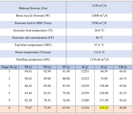
Table 3: Simulation Results of the Temperature(s) and Flowrate(s) Profile of the MSF Process

Makeup flowrate (Fm) 3150 𝑚

3_/ℎ

Brine recycle flowrate (W) 12800 𝑚3/ℎ Seawater feed to MSF (Fsea) 9700 𝑚3/ℎ Seawater feed temperature (Tf) 26.8 °C Seawater salt concentration (CF) 40 °C

Top brine temperature (TBT) 97.6 °C Steam temperature (Tsteam) 112.6 °C

Distillate production (DN) 1270.68 𝑚3/ℎ

Stage No.(j) TB (j) TD (j) TF (j) B (j) D (j) CB (j)

1 94.91 92.99 91.49 12251 46.39 44.63

2 90.42 89.00 88.08 12523 74.89 44.74

3 86.42 85.00 83.58 12439 158.88 45.04 4 83.44 81.01 79.58 12359 238.88 45.33 5 82.28 78.41 76.56 12280 317.89 45.62 6 75.67 72.83 63.94 12164 434.24 46.06

(56)

44 surplus energy from both streams in the heat rejection section. However, the sudden drop would not have happened if the number of stages of both heat recovery and rejection sections increased. Thus, a gradual decrease or increase in temperature and flowrate would be obvious. The results of this analysis are then compared with the results obtained from Abdul-Wahab et al. (2012). Matching results were obtained. From these results, it is evident that the developed model is able to produce robust results.

The flashing brine which enters the first stage of the heat recovery section decreases as it continues flowing to the last stage. This is because of the vapour released from the flashing brine in each stage. While, the distillate flowrate is accumulated as it flows from stage one to last stage, since the vapour is continuously being condensed by the cooling brine to produced distillate. The distillate produced from the MSF plant in this research was 434.24 𝑚3/ℎ (As highlighted in yellow in Table 3). The final distillate reported by the researchers was 1270.68𝑚3/ℎ. Unlike Malik, Bahri and Vu (2016) and Abdul-Wahab et al. (2012) who considered nineteen stages of the MSF plant, this research only covered six stages. Thus, the amount of distillate produced is comparatively lower than the above researchers. This does not mean that the results obtained in this research are invalid as the results obtained were comparatively similar to their findings from stage one to stage six. This demonstrates the accuracy of the developed model.

(57)

45 indicated a similar pattern to various researchers whom have tested this field such as Rosso et al. (1996) and Ali and Kairouani (2016). These results show consistency in line with the works of previous researchers.

The following table (Table 4) exhibits the temperatures and flowrates of the brine heater, mixer, and blowdown. The purpose of the brine heater is to enough temperature to heat the cooling brine, entering the brine heater, at a maximum temperature (TBT) by using steam flowrate. The simulated model displays the obtained values of TBT, steam flowrate, and steam temperature. Overall these findings are in accordance with the findings reported by Malik, Bahri and Vu (2016) and Abdul-Wahab et al. (2012). However, it should be noted that, the TBT reported by Malik, Bahri and Vu (2016) showed a lower optimum value (90℃) as the authors proceeded with optimisation. The authors applied both equality and inequality constraints on optimisation variables including TBT.

Turning now to the mixer process variables, both Malik, Bahri and Vu (2016) and Abdul-Wahab et al. (2012) studies did not report the temperature leaving the mixer and the concentration of the cooling brine. Whereas, in the current research, these variables were included to further explore and understand the behaviour of the process system. This will in turn strengthen the developed model.

Similar to the TBT, Malik, Bahri and Vu (2016) also set equality constraints on the recycle flowrate which was obtained at 9005 (𝑚3/ℎ). On the other hand, the current study showed a higher value at 9298 (𝑚3/ℎ).

(58)

46

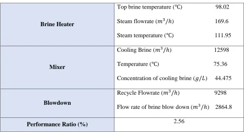
Table 4: Temperatures and Flowrates of the Brine Heater, Mixer, and Blowdown

Brine Heater

Top brine temperature (℃) 98.02 Steam flowrate (𝑚3/ℎ) 169.6 Steam temperature (℃) 111.95

Mixer

Cooling Brine (𝑚3/ℎ) 12598 Temperature (℃) 75.36 Concentration of cooling brine (𝑔/𝐿) 44.475

Blowdown

Recycle Flowrate (𝑚3/ℎ) 9298 Flow rate of brine blow down (𝑚3/ℎ) 2864.8

Performance Ratio (%) 2.56

Table 5 demonstrates results for thermo-dynamic losses and thermos-physical properties of the brine, steam, and water. The overall Heat transfer coefficient (U) and the log mean temperature (LMTD) are presented as well.

(59)

47 fact that the thermodynamic losses have the potential to affect the performance of the MSF plant, the insignificant change of thermodynamic losses does not warrant for any concern.

In each stage, the specific heat capacity of the flashing brine (SBj) shows similar results obtained for the specific heat capacity of the distillate (SDj). Although both concentration and temperature change in each stage, there was a minimal change in thermo-physical properties. Helal et al. (2003) made an assumption that the specific heat capacity of the flashing brine is a weak function of brine concentration. Thus, the results of the current research found clear support to the assumption made by Helal et al. (2003).

Log mean temperature difference (LMTD) defines the temperature driving force between the hot and cold streams in tube heat exchangers (Thulukkanam 2000) . The LMTD results display slight fluctuations between stage one and stage five. However, between stage five and stage six, there was a drastic increase of the LMTD. This is due to the substantial difference in the temperature leaving stage five (TDj) and the feed temperature of the cooling seawater at stage six (TFj). Equation (38) used to determine the LMTD is given in chapter 5, subsection 5.3. The values obtained at stage five was 6.1385 °C as compared to 22.592 °C in stage six (as illustrated in Table 5, highlighted in yellow). These findings have a similar pattern to Mabrouk (2013) results.

(60)

48 presented similar patterns to Rosso et al. (1996) and Mabrouk (2013) results. Under these circumstances, the developed model has been validated against the results reported by other researchers.

Table 5: Results for Thermo-dynamic Losses and Thermo-physical Properties

Thermodynamic Losses Thermo-physical properties Other parameters

Stage No. (j)

BPE (j)

(𝟏 ∗ 𝟏𝟎−𝟑₎ NEA (j) ∆ (j) SB (j) SD (j) Scr (j) LMTD(j) U(j)

1 2 3 4 5 0.6819 0.6787 0.6768 0.6755 0.6753 7.10e-04 7.49e-04 8.60e-04 0.001 0.0014 0.967 1.05 1.1403 1.238 1.306 4.1727 4.1727 4.1728 4.1729 4.1729 4.1745 4.1745 4.1746 4.1747 4.1748 3.976 3.975 3.973 3.971 3.970 2.8814 2.5418 2.9886 2.6581 6.1385 2.885e03 2.844e03 2.789e03 2.738e03 2.698e03

6 0.6707 0.0013 1.46 4.159 4.1748 3.986 22.592 3.074e03

Note: The graphs of the simulation results found in Table 3, 4 and 5 are enclosed in Appendix A.

5.3 Hybrid System (MSF-RO)

(61)

49 As reported earlier, the distillate produced from the stand-alone MSF process was 434.24

𝑚3_/ℎ_{and permeate attained from the stand-alone RO process was 1400}_𝑚3_/ℎ_{. Both} processes are now integrated to increase the final freshwater product. The final product of the hybrid system obtained was 1834.24 𝑚3/ℎ.

Table 6: Simulation Results of the Hybrid MSF-RO Plant

Hybrid MSF-RO

Final Concentration (𝒈/𝑳) Final Product (𝒎𝟑/𝒉)

0.063 1834.24

The final product concentration of the hybrid system is the average of both product concentrations of the stand-alone MSF and RO processes. By integrating product concentration produced from the stand-alone RO (Cp) with salt-free distillate, the salinity of the final product became lower at 0.063 𝑔/𝐿. The results obtained ties well with Malik, Bahri and Vu (2016) findings wherein the authors reported 0.07 𝑔/𝐿 of the final product concentration of the hybrid system.

5.4 Limitations of the Current Thesis

There were several challenges faced throughout the duration of this research. One of the main challenges faced is limited relevant researches performed on the hybrid MSF-RO system. This then leads to the lack of research findings to compare and validate the current thesis. Despite the fact that there were lack of studies on the hybrid system, the challenges were overcome with the in-depth understanding and studies provided by the few researches who attempted to achieve reliable data not only from theoretical studies but also from the actual plant data.

(62)

(63)

51

Chapter 6: Conclusion and Future Work

In this thesis, a steady state mathematical model of the hybrid MSF-RO system has been developed based on material, salt and energy balance. The operating data were gathered from different researches to solve the develop model and ensure data accuracy. The mathematical models of stand-alone systems of MSF and RO were tested individually.

For the stand-alone MSF system, the stimulation results when compared with Abdul-Wahab et al. (2012) and Malik, Bahri and Vu (2016) findings indicate matching results. The current research also considers actual calculations of thermodynamic losses and thermo-physical properties for each stage, of which many researches ignored. Thermo-physical properties are calculated as a function of temperature and concentration. While, thermodynamic losses are calculated as a function of temperature, concentration and other parameters (refer to chapter 4). The results yield positive outcomes of the distillate temperature profile (refer to chapter 5). Moreover, the brine concentration profile has been calculated. With regards to the performance ratio of the MSF, the results indicate that as the number of stages increases, the performance ratio increases. Overall, these values show consistent outcomes when compared to other researches.

(64)

52 For the hybrid MSF-RO, the result shows a reduction in permeate concentration produced by RO system when integrated with MSF plant. Therefore, the final concentration of the hybrid system is the average of both product concentration of stand-alone systems (MSF and RO). Moreover, the final product flow rate is higher as the distillate and permeate flow are combined. The final product concentration of 0.063 g/L is obtained and compared with Malik, Bahri and Vu (2016) where the authors’ final concentration of hybrid system is 0.07 g/L.

While most studies focused on optimisation of the hybrid MSF-RO, these studies are still lacking. On the control design, there were limited research emphasising on the control of the hybrid system. The works presented in this thesis have proven that further research should be performed on the hybrid MSF-RO model for the purpose of optimisation and control design. Moreover, the performance of the hybrid system can be further explored by increasing the number of stages. This will in turn increase the final freshwater product and the final concentration can be further improved. The developed model in this thesis is accurate and promising since the outcomes obtained are validated against other researchers. Ultimately, future researchers are encouraged to improve the model and bring it to the next level.