ORIGINAL ARTICLE
Crosswind Stability Evaluation
of High-Speed Train Using Different Wind
Models
Mengge Yu
1*, Rongchao Jiang
1, Qian Zhang
1and Jiye Zhang
2Abstract
Different wind models are being used for the operational safety evaluation of a high-speed train exposed to cross-winds. However, the methodology for simulating natural wind is of substantial importance in the wind–train system, and different simplified forms of natural wind result in different levels of accuracy. The purpose of the research in this paper is to investigate the effects of different wind models on the operational safety evaluation of high-speed trains. First, three wind models, namely, steady wind model, gust wind model, and turbulent wind model, are con-structed. Following this, the algorithms for computing the aerodynamic loads using the wind models are described. A multi-body dynamic model of a vehicle is then set up using the commercial software “Simpack” for investigating the dynamic behavior of a railway vehicle exposed to wind loads. The rollover risks corresponding to each wind model are evaluated by applying the definition of characteristic wind curves (CWC). The results indicate that the CWC computed using the gust wind model is marginally higher than that computed using the turbulent wind model; the difference is less than 1%. With regard to the steady wind model, the assurance coefficient substantially affects the final CWC. A reasonable agreement of CWC between the steady wind model and turbulent wind model can be obtained by apply-ing an “appropriate value” of the assurance coefficient. This study included a systematic analysis of the operational safety evaluation results using different wind models; the analysis can serve as a reference basis for different engineer-ing accuracy requirements.
Keywords: Crosswind, Railway vehicle, Wind model, Rollover risks, Characteristic wind curves
© The Author(s) 2019. This article is distributed under the terms of the Creative Commons Attribution 4.0 International License (http://creat iveco mmons .org/licen ses/by/4.0/), which permits unrestricted use, distribution, and reproduction in any medium, provided you give appropriate credit to the original author(s) and the source, provide a link to the Creative Commons license, and indicate if changes were made.
1 Introduction
The aerodynamic loads of railway vehicles exposed to strong crosswinds can significant impact the operational safety of railway vehicles. This is because they can modify the operational stability of vehicles by increasing the risk of overturning, e.g., the recent accidents in China, Japan, Belgium, and Switzerland. The crosswind effects become particularly critical at high operating speeds [1–3]. Over the last 30 years, a large number of studies have been conducted in the railway industry to develop methodolo-gies capable of evaluating the level of safety of a railway vehicle in terms of overturning risk.
The assessment of the crosswind stability of railway vehicles is divided into the determination of the aero-dynamic coefficients and the vehicle aero-dynamic charac-teristics. The most common methods for computing the aerodynamic loads are wind tunnel tests on reduced scale models [2, 4–6] and CFD tools [7–9]. Whereas wind tunnel tests yield highly reliable values of the measured forces, CFD tools reduces the cost of detailed studies of phenomena, such as the pressure field and velocity map of flow. The wind data and aerodynamic coefficients are then input into a model of the wind–vehicle system. Gen-erally, a static approach, wherein aerodynamic forces at static equilibrium act on the vehicle, is used owing to its simplicity and the limited number of input data required [10]. However, this method is considered less precise with respect to other available methods such as a multi-body dynamic approach in the time domain, which is
Open Access
*Correspondence: [email protected]
1 College of Mechanical and Electronic Engineering, Qingdao University,
Qingdao 266071, China
capable of accounting for the nonlinear effects of the vehicle dynamics and wind–train interaction [11]. The final output of both the approaches is the characteristic wind curves (CWC), which is the set of characteristic wind speeds that the rolling stock can withstand before certain wheel unloading limit values are exceeded. These curves can then be used to calculate the risk of a wind-induced accident on a particular route and to develop suitable remedial measures.
A suitable construction of the wind model is widely considered critical for effectively assessing the overturn-ing risk of a railway vehicle exposed to crosswinds. The construction of the wind model has a number of levels of complexity, ranging from the simple assumption of a steady wind to a more complex gust of a specific form (such as the Chinese hat gust) and a complete stochastic wind simulation that produces turbulent fluctuations of the correct magnitude and scale. In most previous stud-ies, the crosswind stability analysis of railway vehicles was based on the steady wind hypothesis, and a num-ber of effective results have been obtained. Krajnović et al. [12] used large eddy simulation to study the flow around a simplified train model exposed to crosswind; an overshoot of approximately 30% observed in the yaw-ing moment coefficients indicated the importance of performing dynamic tests for fulfilling safety standards. Giappino et al. [10] compared the crosswind behavior on a high speed train and that on a low speed train through two subsequent analyses: measurement of the aerody-namic coefficients through wind tunnel tests on scale models and evaluation of the rollover risks by applying the definition of CWC based on static equilibrium. The steady wind hypothesis is convenient for either of wind tunnel test or CFD simulation. Furthermore, natural winds were represented as a gust of a specific form. Car-rarini [13], Wetzel and Proppe [14] set up an artificial gust model, considered the most influential but uncer-tain parameters (gust factor, gust length, and aerody-namic coefficients) as stochastic variables, and proposed a reliability analysis method for the crosswind stability of railway vehicles. In EN 14067-6 [15], the construction of a Chinese hat gust wind model and the corresponding assessment methods for the railway vehicle are described. However, simulations of a steady wind and an ideal gust are generally substantially simpler than real-world cases. When a moving vehicle is subjected to crosswind, the aerodynamic loads acting on the vehicle depend on the mean value of the relative wind–vehicle velocity as well as on the statistical properties of the wind [16]. There-fore, certain researchers proposed an alternative proce-dure, i.e., the turbulent wind model; it has spectral and correlation statistics similar to those of natural wind. The stochastic approach is used for studying realistic
wind–train interactions; it can reproduce the interaction between the train dynamics and the aerodynamic loads based on statistical methodology [17–19]. However, to obtain the statistical characteristics of the CWC, a large number of samples are required; this results in substan-tial amount of calculation.
Based on the discussion above, all the three wind mod-els have been used to evaluate the overturning risk of a railway vehicle and many effective results have been obtained. Each approach has its advantages and disad-vantages. It is considered that the turbulent wind model enables an accurate reproduction of the real interaction between the vehicle dynamics and natural wind. Mean-while, the stochastic approach is the most costly and time-consuming. The steady wind model is the simplest and most affordable; however, this approach does not effectively reveal the fluctuation characteristics of natural wind. Different simplified forms of natural wind results in different levels of accuracy of the operational evalua-tion results; furthermore, certain simplified approaches are likely to yield highly inaccurate results. Although certain researchers have described the accuracy of the wind models, the analysis and conclusion are generally approximate and qualitative. The differences in the oper-ational safety evaluation results obtained using different wind models need to be quantified to determine the best trade-off between accuracy and amount of calculation. This requires a systematical analysis of the differences in the operational safety evaluation results of different wind models, including those with regard to the simplified form of natural wind, aerodynamic force, dynamic safety index, and CWC.
The purpose of the present study is to investigate the influence of different wind models on the crosswind sta-bility evaluation of high-speed train. In Section 2, the construction of the steady wind model, gust wind model, and turbulent wind model are described in detail; the parameters in the wind model are also specified. In Sec-tion 3, the computational algorithms of the aerodynamic force and moment using different wind models are devel-oped. In Section 4, a multi-body dynamic vehicle model with measured track irregularities is developed to com-pute the safety index of a high-speed train exposed to aerodynamic loads; the methodology of crosswind stabil-ity assessment is also presented in this section. The simu-lation results are discussed in Section 5.
2 Wind Model
train is the lowest when the wind flows approximately in the normal direction [20, 21]. Therefore, in this study, variations in the wind direction are not considered, and only the pure crosswind, i.e., wind perpendicular to the track, is considered.
2.1 Steady Wind Model
In most of the early research on crosswind stability, nat-ural wind is assumed to be steady wind. Moreover, the wind speed in the steady wind model is assumed to be the peak value of natural wind; this is expressed as
where wˆ is the peak wind speed, w¯ is the mean wind speed, σw is the standard deviation of natural wind speed,
and k is the assurance coefficient. The different values of k correspond to the different assurance rates; an assur-ance rate is defined as the probability that the peak wind speed does not exceed w¯ +kσw . For example, in the case of a Gaussian distribution, k= 2 implies that the prob-ability that the peak wind speed does not exceed w¯ +2σw is 97.72%; when k= 2.84, the probability that the peak wind speed does not exceed w¯ +2.84σw is 99.77%.
The standard deviation of wind speed depends mainly on the mean wind speed and turbulence intensity; it is calculated by the following equation:
where Iz is the turbulence intensity and can be computed by the following equation [14]:
where h is the height above the ground and h0 is the ground roughness length. According to EN 14067-6 [15], h = 4.0 m, h0= 0.07 m.
2.2 Gust Wind Model
Gust scenarios are utilized to model certain extreme wind conditions without the need to wait for the normal turbu-lent wind process to occur [14]. The most realistic wind simulation is a spatial and time-dependent wind field through which the train would pass. It is assumed that the train speed is constant; thus, the temporal distribution can be evaluated from the spatial one by transformation. An ideal gust is a simplified form of real unsteady wind, which involves a variation in the wind velocity defined by a simple, generally analytical function of time. In practice, different gust shapes are used; the most common are expo-nential gust shape, “1-cos” gust shape, ramp gust shape, and step gust shape. The exponential shape is the most advanced model available; this is because it is not empirical
(1)
ˆ
w= ¯w+kσw,
(2) σw=Izw,¯
(3) Iz= 1
ln(h/h0)
1− 5
105
log
h
0
0.05
+2 7
,
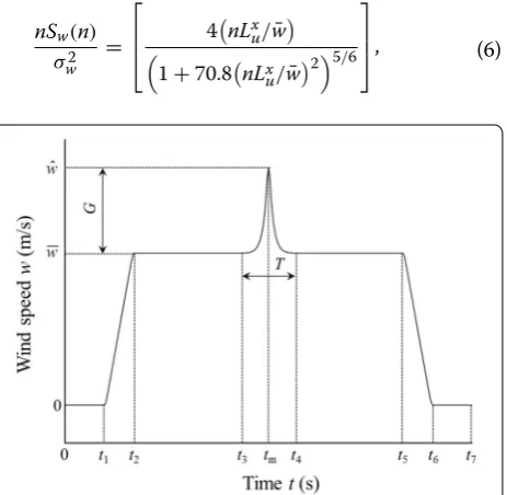
and is obtained by analyzing real wind data. In EN 14067-6 [15], a Chinese hat gust wind model, which is more or less an example of the exponential shape, is depicted specifi-cally (Figure 1).
According to the frozen turbulence hypothesis, a gust does not evolve and is transported with the mean wind speed w¯ ;
¯
w is assumed to be constant. A complete Chinese hat gust wind can be described by a form of piecewise function; the emphasis is on describing the fluctuating component of the gust wind. The gust factor G and gust duration T are two main characteristic parameters to describe the gust wind.
The gust factor G is defined as the ratio between the peak value wˆ and mean value w¯ of the wind speed:
According to EN 14067-6 [15], the gust factor G in the present study is 1.6946; the corresponding assurance coef-ficient k is 2.84.
The gust duration T describes the duration of the gust (see Figure 1). It can be calculated from the turbulence power spectral density of the natural wind speed, which is given by (EN 14067-6, 2010):
where n is the frequency, n1 is the integrated lower limit of the frequency, n2 is the integrated upper limit of the frequency, and Sw(n) is the turbulence power spec-tral density of the natural wind speed. According to EN 14067-6 [15], n1= 1/300, n2= 1. The von Karman spectral is used in this study; it is calculated from [22]
(4) G= ˆw/w¯ =1+kIz.
(5) T = 1
2 n2
n1 n2Sw(n)dn n2
n1 Sw(n)dn −0.5
,
(6)
nSw(n) σ2
w =
4� nLxu/w¯� �
1+70.8� nLx
u/w¯
�2�5/6
,
where Lxu is the longitudinal integral length scale and can
be computed by the following equation [15]:
The characteristic frequency of gust is denoted as f; its computational formula is
The wind speed normal to the vehicle along the track can be calculated from
where x˜ represents the distance along the track toward the position of the maximum amplitude of the gust wind; its computational formula is
where tm represents the time corresponding to the maxi-mum amplitude of the gust wind. As shown in Figure 1, after t3, the increase follows the mirrored Chinese hat until t4. For practical implementation, the exponential decay is assumed to achieve the lower limit w¯ after a
maximum deviation of 1% is attained between those two values.
The wind gust time history is low-pass filtered using a moving spatial average based on a window size equal to the vehicle length and a step-size less than 0.5 m [15]. Owing to this filtering, the simulated peak wind speed of the gust wind is less than the assumed peak value wˆ.
2.3 Turbulent Wind Model
In a turbulent wind model, a spatial-time distribution of the wind speed is constructed; this enables the reproduc-tion of the physical stochastic characteristics of natural winds. A complete stochastic simulation of the winds can be characterized in terms of a wind with the mean veloc-ity and a fluctuating velocveloc-ity. The instantaneous wind velocity can be expressed as follows:
where w′ is the fluctuating wind speed. The fluctuat-ing wind speed is a stochastic process with a normal distribution.
We assumed that the train moves at a constant veloc-ity v toward the terminal on the straight rail line and that the turbulent wind velocity is horizontal and per-pendicular to the track. Only the along-wind compo-nent, i.e., the longitudinal compocompo-nent, is considered in this study. This component represents the promi-nent part of wind fluctuations [15]. To account for the
(7)
Lxu =50h
0.35
h0.0630 .
(8)
f = 1
2×4.1825T.
(9) w= ¯w+2.84σwe−16fx/˜ w¯,
(10) ˜
x=v|t−tm|, t∈[t3,t4],
(11) w= ¯w+w′,
aerodynamic effects of the turbulent wind, an unsteady crosswind field as experienced by the train needs to be generated. Two main approaches for turbulent wind generation have been developed over the past few years. One of the methods commonly used is to numerically simulate the wind time-histories at a large number of points, separated by short distances, along a track [17, 19]. The time series at each point exhibits the correct spectral characteristics; moreover, the correla-tions between the time series at adjacent points exhibit statistics that are consistent with those measured at full scale. Another method is to simulate a wind time-series of a moving reference point coincident with the vehicle at a particular instant; this method is applied in this study. It is carried out by decomposing the wind spectrum relative to the moving train into a series of sinusoidal velocity variations of random phase and then combining these time series into unsteady velocity time series at the train’s position [22, 23]. The Cooper theory defines the dimensionless power spectral density func-tion for the wind speed at a moving point [22]:
where
where nSw/σw2 is the dimensionless power spectral den-sity, Sw is the power spectral density, Lyu is the lateral inte-gral length scale, and u¯ is the mean wind velocity relative
to the train ( u¯ =√v2+ ¯w2).
The lateral integral length scale Lyu can be computed by the following equation [15]:
The wind velocity time series w′ at the position of the train are reproduced using the method of harmonic superposition [24]:
where t is the time, nj is the frequency step, and rj is a random number between zero and one.
(12) nSw
σw2 =
4�nL′u/u¯� �
1+70.8� nL′
u/u¯ �2�5/6
· �� ¯ w ¯ u �2 + � 1− � ¯ w ¯ u �2�
0.5+94.4�
nL′u/u¯�2
1+70.8� nL′
u/u¯ �2
� .
(13) L′u =Lxu
� ¯ w ¯ u �2 +4 � Lyu Lx u
�2� 1− � ¯ w ¯ u
�2�
0.5
,
(14) Lyu =0.42Lxu.
(15) w′=
j
3 Aerodynamic Forces and Moments
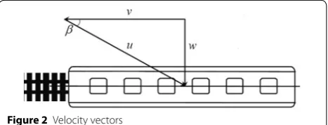
Figure 2 shows a velocity diagram that relates the wind speed w, vehicle speed v, and the wind direction relative to the moving train β . β is named as “yaw angle” in this study.
The wind speed relative to the train u is expressed as
The yaw angle β is expressed as
For the steady wind model, the wind speed w is assumed to be an invariant value wˆ ; it is computed by Eq. (1). It is demonstrated that u and β are invariant if the vehicle speed stays constant. In that analysis, the steady aerodynamic forces and moments are commonly computed using aero-dynamic coefficients as follows:
where F is the aerodynamic force, M is the aerodynamic moment, CF is the aerodynamic force coefficient, CM is the aerodynamic moment coefficient, ρ is the density of air, A is the reference area, and h is the reference height. In the following, A = 10 m2 and h= 3 m is adopted [15].
For the Chinese hat gust wind model, both β and u are time-varying owing to the unsteady nature of the wind gusts. The wind speed w in Eqs. (16) and (17) is com-puted by Eq. (9). According to the quasi-steady theory, in the condition of gust wind, the aerodynamic force and aerodynamic moment are evaluated by Eqs. (20) and (21), respectively:
The quasi-steady assumption mentioned above assumes that the fluctuations in the force induced on the train occur directly because of the turbulence in the (16)
u2=v2+w2.
(17)
tanβ = w
v.
(18) F = 1
2ρACF(β)u 2,
(19) M= 1
2ρAhCM(β)u 2,
(20) F(t)= 1
2ρACF(β(t))u(t) 2,
(21) M(t)= 1
2ρAhCM(β(t))u(t)
2.
approaching wind. Although the quasi-steady assump-tion is effective in numerous circumstances, it does not hold completely for the turbulent wind model. The force fluctuations do not completely follow the velocity fluctu-ations because the small-scale turbulence in the oncom-ing wind is not completely correlated over the entire exposed area of a train vehicle. An alternative approach is the corrected steady theory; herein, the quasi-steady theory is applied and corrected with the admit-tance function [16].
According to the corrected quasi-steady theory, in a condition of turbulent wind, the aerodynamic force and aerodynamic moment are evaluated by Eqs. (22) and (23), respectively:
where uc is the corrected wind speed relative to the train and βc is the corrected yaw angle; these can be computed by Eqs. (24) and (25), respectively
where wc′ is the corrected fluctuating wind speed. The corrected fluctuating wind speed w′c is
where Swc is the power spectral density corresponding to the corrected wind speed w′c.
Swc can be computed by the following equation:
where χ2 is the aerodynamic admittance function. Baker [23] assembled a significant amount of experi-mental data from a variety of full scale and wind tunnel tests on a variety of trains and provided a simple expres-sion for the aerodynamic admittance function used on railway trains:
where ns is the dimensionless frequency; n′=sinβ¯ , β¯ is the mean yaw angle, =2.0 for the side force coefficient, and =2.5 for the lift force coefficient.
(22) F(t)= 1
2ρACF(βc(t))uc(t) 2,
(23)
M(t)= 1
2ρAhCM(βc(t))uc(t) 2,
(24)
u2c=v2+ ¯
w+wc′2
,
(25)
βc=atan¯
w+w′c v ,
(26) wc′ =
j
2Swcnj�nj0.5sin2πnjt+2πrj,
(27)
Swc=χ2Sw,
(28)
χ2= 1
1+(ns/n′)2 2,
The aerodynamic admittance function of the rolling moment is identical to that of the side force. For the yaw and pitch moments, the moment fluctuations are consid-ered to be coincident with the velocity fluctuations [15].
The aerodynamic coefficients, which depend on the yaw angle, can be determined experimentally or numeri-cally. The side force coefficient CFs, lift force coefficient CFl, rolling moment coefficient CMr, yaw moment coeffi-cient CMy, and pitch moment coefficient CMp on the vehi-cle of a Chinese high-speed train are depicted in Figure 3
[25, 26].
4 Vehicle Dynamic Model
4.1 Multi‑Body Dynamic Model
To evaluate the dynamic behavior of a vehicle subjected to crosswind action, complex dynamic methodologies are developed in the time domain. The aerodynamic loads are then input into the model of the wind–vehicle sys-tem to compute the vehicle dynamic characteristics. In EN14067-6 [15], a simple three-mass model with no rep-resentation of vehicle suspension, and a more complex five-mass model with suspension stiffness are modelled based on static equilibrium. In this study, a method of further complexity, i.e., the time-dependent multi-body simulation (MBS) of a vehicle, is used to determine the vehicle dynamics or wind–train interaction.
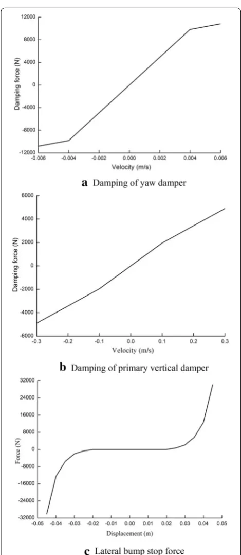
A multi-body dynamic model of a Chinese high-speed driving trailer has been constructed using the highly sophisticated commercial software SIMPACK. It consists of 15 rigid bodies (car-body, bogies, wheelsets, tumblers etc.), an accurate description of the wheel/rail contacts, a nonlinear spring and damper forces, and bump stops. The 15 rigid bodies are connected with springs and dashpots, forming a vehicle subsystem of 50 degrees-of-freedoms
[26]. The nonlinear dynamic characteristics of the sus-pension systems, such as the damping of the yaw damper, damping of the primary vertical damper and lateral bump stop force, are shown in Figure 4. The wheel–rail inter-action and rail irregularities are significant components
Figure 3 Aerodynamic coefficients
of the vehicle dynamic model. The LMA wheel and T60 Rail [27] are adopted in the multi-body simulation. The measured track spectrum of the Beijing–Tianjin intercity high-speed railway in China is adopted as the rail irregu-larity in the simulation.
After the vehicle dynamic model is set up, the aerody-namic loads (discussed in Section 3) are applied at the aerodynamic reference point on the car-body to compute the safety index. Although this approach has not been verified for the vehicles, it is a reasonable approximation recommended by a number of previous investigations [2,
13].
4.2 Operational Safety Evaluation
The final aim of the wind stability analysis is to evalu-ate the operational safety of the high-speed train. In this regard, the load reduction factor is considered to be an important safety index. This index is considered ineffi-cient and over-conservative. Nonetheless, it is still widely used owing to its simplicity and the fact that wheel forces can be experimentally measured on real driving vehicles [13, 15, 21, 26]. It is defined as
where P is the wheel load reduction amount and P¯ is the average wheel load of the left wheel and right wheel. The time history of this index is to be filtered through a 2 Hz low-pass filter.
The final output of the operational safety evaluation of the high-speed train is the CWC, which is defined as the wind-speed limit beyond which the vehicle’s safety lim-its (e.g., the load reduction factor) are exceeded. For the steady wind model and gust wind model, the CWC could be uniquely determined according to the specified input parameters. However, for the turbulent wind model, as the wind is a random process, when the stochastic methodol-ogy is used for evaluation, different time histories of wind velocities satisfying identical statistical properties (such as the mean wind speed and turbulence intensity) are gener-ated; this results in different time histories of the aerody-namic loads and load reduction factor for identical wind scenarios. As a result, a series of CWCs will be generated for identical wind scenarios. Therefore, it is necessary to understand the statistical properties of CWC. Through the statistical analysis, the mean value and standard deviation of the CWC can be obtained; then, the spread range S of the CWC is defined as [15]
where µCWC is the mean value of CWC and σCWC is the standard deviation of CWC. For the Gaussian
(29)
�P/P¯ <0.8,
(30) S=µCWC±2σCWC,
distribution, 2σCWC corresponds to 95.45%; i.e., the prob-ability that the CWC lies in the spread range S is 95.45%.
5 Numerical Simulation Analysis
5.1 Wind and Force Characteristics
In the simulation, the train speeds are 200 km/h, 250 km/h, 300 km/h, and 350 km/h; furthermore, the mean wind speeds are 10 m/s, 15 m/s, 20 m/s, 25 m/s, 30 m/s, and 35 m/s. For the simulation of gust wind, the gust factor is 1.6946, the height above the ground is 4.0 m, and the ground roughness length is 0.07 m. For the simulation of turbulent wind, the simulated frequency range is [0.001 Hz, 10 Hz], the frequency step is 0.001 Hz, and the total superposition number is 10000. The wind speeds are generated every 0.05 s, and 10 min realizations of the time series are processed. Given the wind time his-tories, the method presented in Section 3 is used to simu-late the aerodynamic forces and moments of high-speed trains. The aerodynamic forces and moments are then input into the multi-body dynamic model established in Section 4, to simulate the dynamic behavior of the train. Finally, the outputs are processed to evaluate the safety index and then to assess the operational safety.
To verify the accuracy of the wind simulation, the cur-rent spectrum obtained from the simulated wind time series are compared to the target spectrum. Figure 5
shows the comparison of the fluctuating wind spectrum for a vehicle speed of 350 km/h and a mean wind speed of 20 m/s. The results reasonably agree with the target spectrum across a significant portion of the frequency domain.
Figure 6 shows an example of simulated gust wind time-history for a vehicle speed of 350 km/h and a mean wind speed of 20 m/s. For comparative analysis, the steady winds with assurance coefficients of 2 and 2.84 for a mean wind speed of 20 m/s are also marked in Figure 6.
From Eq. (1), the assurance coefficients of 2 and 2.84 cor-respond to peak wind speeds of 29.78 m/s and 33.89 m/s, respectively. As is illustrated in Figure 6, because of the low-pass filtering, a maximum gust wind speed of 31.32 m/s is observed; this is smaller than the unfil-tered peak value of 33.89 m/s computed by Eq. (4). From the perspective of maximum wind speeds, the assurance coefficients of 2 and 2.84 in the steady wind model are not consistent with those of the gust wind model.
Figure 7 shows an example of a simulation of turbulent wind time-history, for a vehicle speed of 350 km/h and a mean wind speed of 20 m/s. The two horizontal lines in Figure 7 convey a concept similar to that in Figure 6. During the 600 s, a few of the random values of the wind speed exceed 29.78 m/s (corresponds to the assurance coefficient of 2); furthermore, the probability that the maximum wind speed does not exceed 29.78 m/s, calcu-lated by statistics analysis, is 97.98%; this is approximately equal to the theoretical value (97.72%) mentioned in
Section 2.1. Similarly, the probability that the maximum wind speed does not exceed 33.89 m/s (corresponds to the assurance coefficient of 2.84), calculated by statis-tics analysis, is 99.68%; this is approximately equal to the theoretical value (99.77%) mentioned in Section 2.1.
Figure 8 shows the comparison of the turbulent wind time-history and gust wind time-history. The result in Figure 8 indicates that the variation in the gust wind could effectively reflect the fluctuating characteristics of the turbulent wind. The gust wind model approximates a random process in the vicinity of the local maximum and gust duration (the mode of the distribution).
Figure 9 shows a plot of the simulated aerodynamic side force computed by the gust wind model for a vehi-cle speed of 350 km/h and a mean wind speed of 20 m/s. For comparative analysis, the aerodynamic side forces computed by the steady wind model with assurance coef-ficients of 2 and 2.84 for a mean wind speed of 20 m/s are also marked in Figure 9. As is illustrated in Figure 9, Figure 6 Time history of gust wind
Figure 7 Time history of turbulent wind
Figure 8 Comparison of turbulent wind and gust wind
because of the low-pass filtering of gust wind, the maxi-mum aerodynamic side force is 118.83 kN; this is smaller than 132.06 kN (corresponding to the wind speed of 33.89 m/s). With regard to the steady wind model, the simulated aerodynamic side forces are 111.23 kN and 132.06 kN corresponding to the assurance coefficients of 2 and 2.84, respectively.
Figure 10 shows, as an example, the time history of the aerodynamic side force computed by the turbulent wind model for a vehicle speed of 350 km/h and a mean wind speed of 20 m/s. The two horizontal lines in Figure 10
convey a concept identical to that in Figure 9. Figure 10
shows that the simulated unsteady side forces computed by the turbulent wind model are significantly smaller than 132.06 kN; furthermore, the probability of the unsteady side forces larger than 111.23 kN is also highly marginal. Owing to the influence of the aerodynamic admittance function, the force calculation effectively yields a weighted average of the force from the previous time. Thus, the simulated force damps out the high fre-quency fluctuations in the turbulent wind. Moreover, as the turbulent wind is a stochastic process with a normal distribution, the unsteady aerodynamic loads of the high-speed train are also approximately normally distributed [21, 25].
Figure 11 shows the comparison of the aerodynamic side force computed by the turbulent wind model and gust wind model for a vehicle speed of 350 km/h and a mean wind speed of 20 m/s.
Figure 11 shows that the maximum aerodynamic side force computed by the gust wind (118.83 kN) is approxi-mately equal to that computed by the turbulent wind (119.65 kN).
5.2 CWC Evaluation
For the steady wind model and gust wind model, the load reduction factor could be uniquely determined according to the input conditions. However, for the turbulent wind Figure 10 Aerodynamic side force for turbulent wind Figure 11 Comparison of aerodynamic side force for turbulent wind
and gust wind
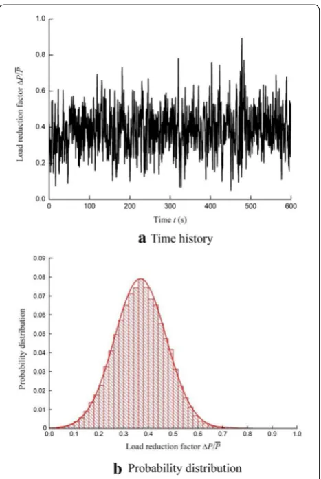
model, as the wind is a random process, different time histories of the load reduction factor will be obtained for identical wind scenarios. Therefore, the statistical charac-teristics of the load reduction factor should be discussed. Figure 12 shows, as an example, a typical time history of the load reduction factor and its probability distribution computed by the turbulent wind model for a vehicle speed of 350 km/h and a mean wind speed of 20 m/s. As is pre-sented in Figure 12, the load reduction factor computed by the turbulent wind model exhibits stochastic characteris-tics and can be effectively fitted with a normal distribution. Through the statistical analysis, the mean value and stand-ard deviation of the load reduction factor can be obtained.
The maximum value of the load reduction factor is used to evaluate the wind stability of the high-speed train. Thus, the extreme value distribution of the load reduction factor is discussed below. The permissible value of the load reduc-tion factor specified in Chinese design guideline is 0.8, as mentioned in Eq. (29). As illustrated in Figure 12, the load reduction factor is approximately normally distributed. To facilitate explanation, the load reduction factor is repre-sented as X(t) , which is normally distributed. Assume that the maximum value of X(t) is Xmax for the continuous time T; its mean value and standard deviation are expressed by Eqs. (31) and (32) respectively [28]:
where µXmax is the mean value of Xmax , σXmax is the standard deviation of Xmax , γ is the Euler constant ( γ =0.5772 ), µX is the mean value of X(t) , and σX is the standard deviation of X(t) . ν can be computed by the fol-lowing equations:
where SY is the power spectral density of Y(t).
Figure 13 shows an example of a simulated maximum value of the load reduction factor as a function of the mean
(31) µXmax=µX+
2 ln(νT)+ √ γ 2 ln(νT)
σX,
(32) σXmax=
π √ 6
1 √
2 ln(νT)σX,
(33)
ν= 1 2π
m2 m0 ,
(34)
m0=
∞
0
SY(n)dn,
(35)
m2=
∞
0
n2SY(n)dn,
(36) Y(t)= X(t)−µX
σX ,
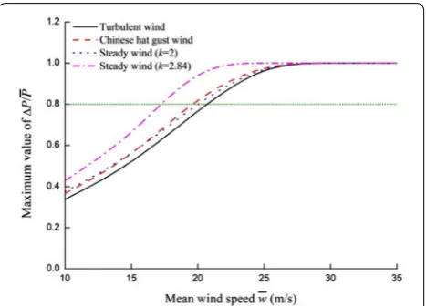
wind speed, using different wind models, for a vehicle speed of 350 km/h. The horizontal dotted line in Figure 13
represents the limit value of the load reduction factor. The intersection of the dotted line with the curves repre-sents the maximum mean wind speed the train could be exposed to without derailment. However, for the turbulent wind model, a series of curves of the load reduction fac-tor, all corresponding to the same wind scenario and same vehicle speed, are obtained owing to its stochastic nature. Therefore, for the turbulent wind model, the data pro-vided in Figure 13 are the mean values of the maximum values of the load reduction factor; the standard deviation is shown in Figure 14. As shown in Figures 13 and 14, if the assurance coefficient is 2, the load reduction factor com-puted by steady wind model is approximately equal to that computed by gust wind model. However, if the assurance coefficient is 2.84, the load reduction factor is significantly larger than that computed by gust wind model. With
Figure 13 Maximum value of load reduction factor
regard to the turbulent wind model, because of the effects of the stochastic characteristics, it is challenging to con-clude whether the results are larger or smaller than those computed by the other two models.
The final CWCs evaluated by means of the different wind models are shown in Figure 15. For the turbulent wind model, the mean value, upper bound, and lower bound of the spread range S of the CWC are provided. Figure 15 shows that for the turbulent wind model, the upper bound of the spread range S of the CWC is appar-ently overestimated. The lower bound of the spread range S of the CWC (μCWC − 2σCWC ) is considered to be more appropriate for evaluating the operational safety of the high-speed train. Because the probability of the CWC in the spread range S is 95.45% in the case of a Gauss-ian distribution, the probability of the CWC less than the lower bound of the spread range S is 2.28%. Figure 15
also shows that the CWC computed by gust wind model is marginally higher than that computed by the turbulent wind model; furthermore, the difference is less than 1%. However, the gust wind model can provide only a simple fixed CWC and cannot evaluate the risk of train derail-ment. The turbulent wind model can provide a more comprehensive evaluation and can effectively evaluate the risk of train derailment. In the case of a rapid prelimi-nary evaluation, the gust wind model can be used. How-ever, for a more comprehensive evaluation, the turbulent wind model is required. With regard to the steady wind model, the CWC is underestimated for an assurance coefficient of 2.84 and overestimated for an assurance coefficient of 2, compared to that computed by the tur-bulent wind model. Therefore, the assurance coefficient is observed to significantly affect the final CWC for the steady wind model.
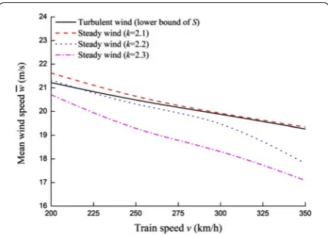
Figure 16 shows the CWCs evaluated by the steady wind model for a variety of assurance coefficients, together with the result evaluated by the turbulent wind model (lower bound of S) for comparison. Figure 16
shows that the CWC computed with steady wind and assurance coefficient of 2.1 is approximately equal to that computed by the turbulent wind model; the difference is less than 2% for the train speeds of 200–350 km/h. These results imply that a relatively accurate assessment result could be obtained if an appropriate value of the assurance coefficient is specified. However, it should be noted that the “appropriate value” of the assurance coefficient could be more or less different for multiple types of vehicles.
6 Conclusions
The topic of the wind stability of high-speed trains has gained substantial attention in the last few years, and the accurate simulation of natural winds is a key issue in the assessment of wind-induced safety. There are three widely used wind models, ranging from the simplest sta-tionary wind to a more complex gust wind and the most realistic turbulent wind. However, the different levels of complexity of the wind models are likely to result in dif-ferent levels of accuracy of the evaluation results. The crosswind stability evaluation of a high-speed train by using different wind models has been investigated in this study. Wind velocity time histories, aerodynamic quan-tities (aerodynamic force time histories), and dynamic quantities (load reduction factor, CWC) for the same mean wind speed are simulated for comparing the three wind models. The results demonstrate that although the simulated time histories of the aerodynamic force com-puted by the gust wind model and turbulent wind model appear to vary significantly, the load reduction factor and the CWCs obtained from the gust wind model are Figure 15 CWC for the three wind models Figure 16 CWC for steady wind model with different assurance
consistent with those from the turbulent wind model across a wide range of train speeds and mean wind speeds. With respect to the steady wind model, which is the simplest form of natural wind, the results depend on the value of the assurance coefficient. According to the examples of this paper, different values of the assur-ance coefficients in the steady wind model result in either underestimated or overestimated results. Therefore, a reasonable agreement of CWC between the steady wind model and turbulent wind model can be obtained if an “appropriate value” of the assurance coefficient is used. For the vehicle studied in this paper, the appropriate value is 2.1. That is, a steady wind model can also pro-vide a relatively accurate assessment of the CWC if an appropriate value of the assurance coefficient is speci-fied. However, it should be noted that the “appropriate value” could be more or less different for various types of vehicles.
Authors’ Contributions
Mengge Yu was in charge of the whole trial. All authors read and approved the final manuscript.
Author Details
1 College of Mechanical and Electronic Engineering, Qingdao University,
Qingdao 266071, China. 2 State Key Laboratory of Traction Power, Southwest
Jiaotong University, Chengdu 610031, China.
Authors’ Information
Mengge Yu, born in 1985, is currently an associate professor at College of Mechanical and Electronic Engineering, Qingdao University, China. She received her PhD degree from Southwest Jiaotong University, China, in 2014. Her research interests include train aerodynamic, vehicle system dynamics.
Rongchao Jiang, born in 1985, is currently a lecturer at College of Mechani-cal and Electronic Engineering, Qingdao University, China. He received his PhD degree from Jilin University, China, in 2016.
Qian Zhang, born in 1985, is currently a lecturer at College of Mechani-cal and Electronic Engineering, Qingdao University, China. He received his PhD degree from China Academy of Railway Sciences, in 2014.
Jiye Zhang, born in 1965, is currently a professor at State Key Laboratory of Traction Power, Southwest Jiaoton University, China. He received his PhD degree from Southwest Jiaotong University, China, in 1998.
Competing Interests
The authors declare that they have no competing interests.
Funding
Supported by National Natural Science Foundation of China (Grant Nos. 51705267, 51605397), China Postdoctoral Science Foundation Grant (Grant No. 2018M630750), Shandong Provincial Natural Science Foundation of China (Grant No. ZR2014EEP002).
Received: 17 November 2017 Accepted: 4 April 2019
References
[1] C Baker, H Hemida, S Iwnicki, et al. Integration of crosswind forces into train dynamic modelling. Proceedings of Institution Mechanical Engineers Part F - Journal of Rail and Rapid Transit, 2011, 225: 154–164.
[2] F Dorigatti, M Sterling, C J Baker, et al. Crosswind effects on the stabil-ity of a model passenger train- A comparison of static and moving
experiments. Journal of Wind Engineering and Industrial Aerodynamics, 2015, 138: 36–51.
[3] F Cheli, F Ripamonti, G Rocchi. Aerodynamic behaviour investigation of the new EMUV250 train to cross wind. Journal of Wind Engineering and Industrial Aerodynamics, 2010, 98: 189–201.
[4] X H He, Y F Zou, H F Wang, et al. Aerodynamic characteristics of a trailing rail vehicles on viaduct based on still wind tunnel experiments. Journal of Wind Engineering and Industrial Aerodynamics, 2014, 135: 22–33. [5] F Cheli, S Giappino, L Rosa, et al. Experimental study on the aerodynamic
forces on railway vehicles in presence of turbulence. Journal of Wind Engineering and Industrial Aerodynamics, 2013, 123: 311–316. [6] G Tomasini, S Giappino, R Corradi. Experimental investigation of the
effects of embankment scenario on railway vehicle aerodynamic coeffi-cients. Journal of Wind Engineering and Industrial Aerodynamics, 2014, 131: 59–71.
[7] A Premoli, D Rocchi, P Schito, et al. Comparison between steady and moving railway subjected to crosswind by CFD analysis. Journal of Wind Engineering and Industrial Aerodynamics, 2016, 156: 29–40.
[8] H Hemida, C J Baker. Large-eddy simulation of the flow around a freight wagon subjected to a crosswind. Computers & Fluids, 2010, 39: 1944–1956.
[9] X M Shao, J Wan, D W Chen. Aerodynamic modeling and stability analysis of a high-speed train under strong rain and crosswind conditions. Journal of Zhejiang University - Science A: Applied Physics & Engineering, 2011, 12: 964–970.
[10] S Giappino, D Rocchi, P Schito, et al. Cross wind and rollover risk on lightweight railway vehicles. Journal of Wind Engineering and Industrial Aerodynamics, 2016, 153: 106–112.
[11] M G Yu, J Y Zhang, K Y Zhang, et al. Study on the operational safety of high-speed trains exposed to stochastic winds. Acta Mechanica Sinica, 2014, 30(3): 351–360.
[12] S Krajnović, P Ringqvist, K Nakade, et al. Large eddy simulation of the flow around a simplified train moving through a crosswind flow. Journal of Wind Engineering and Industrial Aerodynamics, 2012, 110: 86–99. [13] A Carrarini. Reliability based analysis of the crosswind stability of railway
vehicles. Journal of Wind Engineering and Industrial Aerodynamics, 2007, 95(7): 493–509.
[14] C Wetzel, C Proppe. On reliability and sensitivity methods for vehicle systems under stochastic crosswind loads. Vehicle System Dynamics, 2010, 48(1): 79–95.
[15] EN14067-6. Railway applications - Aerodynamics - Part 6: Requirements and test procedures for cross wind assessment. CEN, Brussels, 2010. [16] G Tomasini, F Cheli. Admittance function to evaluate aerodynamic loads
on vehicles: experimental data and numerical model. Journal of Fluids and Structures, 2013, 38: 92–106.
[17] F Cheli, R Corradi, G Tomasini. Crosswind action on rail vehicles: a meth-odology for the estimation of the characteristic wind curves. Journal of Wind Engineering and Industrial Aerodynamics, 2012, 104-106: 248–255. [18] C J Baker. A framework for the consideration of the effects of crosswinds
on trains. Journal of Wind Engineering and Industrial Aerodynamics, 2013, 123: 130–142.
[19] Y Ding, M Sterling, C J Baker. An alternative approach to modeling train stability in high crosswinds. Proceedings of Institution Mechanical Engineers Part F - Journal of Rail and Rapid Transit, 2008, 222: 85–97.
[20] C Baker, F Cheli, A Orellano, et al. Cross-wind effects on road and rail vehicles. Vehicle System Dynamics, 2009, 47(8): 983–1022.
[21] M G Yu, J L Liu, D W Liu, et al. Investigation of aerodynamic effects on the high-speed train exposed to longitudinal and lateral wind velocities. Journal of Fluids and Structures, 2016, 61: 347–361.
[22] R K Cooper. Atmospheric turbulence with respect to moving ground vehicles. Journal of Wind Engineering and Industrial Aerodynamics, 1985, 17(2): 215–238.
[23] C J Baker. The simulation of unsteady aerodynamic crosswind forces on trains. Journal of Wind Engineering and Industrial Aerodynamics, 2010, 98: 88–99.
[24] C Gan. A new procedure for exploring chaotic attractors in nonlinear dynamical systems under random excitation. Acta Mechanica Sinica, 2011, 27(4): 593–601.
[26] M G Yu. Study on the wind-induced safety of the high-speed train based on the reliability. Chengdu: Southwest Jiaotong University, 2014. (in Chinese) [27] D B Cui, L Li, X S Jin, et al. Optimal design of wheel profiles based on
weighted wheel/rail gap. Wear, 2011, 271: 218–226.