R E S E A R C H
Open Access
An improved numerical solution of the
singular boundary integral equation of the
compressible fluid flow around obstacles
using modified shape functions
Lumini¸ta Grecu
**Correspondence: [email protected] Department of Applied
Mathematics, University of Craiova, Craiova, Romania
Abstract
In this work an improved numerical solution of the singular boundary integral equation of the 2D compressible fluid flow around obstacles is obtained by a boundary element method based on modified shape functions and cubic boundary elements. The singular boundary integral equation with sources distribution is considered in this paper, and for its discretization cubic boundary elements are used. The integrals of singular kernels are evaluated using modified shape functions which are deduced by using series expansions for the basis functions we choose for the local approximation models. A computer code is made using Mathcad programming language and, based on it, some particular cases are solved. In order to validate the proposed method, comparisons between numerical solutions and exact ones are performed for the considered test problems. The advantage of using modified shape functions for evaluating the singularities is pointed out through a comparison study between the numerical solution obtained by the method proposed in this paper and the one obtained by using a truncation method for evaluating the singularities.
MSC: 65N38; 76M15; 76G25; 35Q35
Keywords: discretization; boundary element method; cubic boundary element; singular boundary integral equation; modified shape functions
1 Introduction
When solving problems of real life described by partial differential equations or systems of partial differential equations with boundary conditions, seldom this can be done an-alytically, and so, in order to find an approximate solution, numerical techniques, such as: the finite difference method, the finite element method, the finite volume method, the boundary element method, and others, have to be applied.
Among these methods the literature highlights the boundary element method because of its advantages over the other, especially when dealing with fluid flows around obsta-cles, in fact with problems with infinite domains. The reduction by one of the problem’s dimension, less nodal values need to be found, a reduced computational effort is needed, obtaining an exact boundary formulation of the problem, are only some of these advan-tages, presented in many books dedicated to this method (as, for example, [–]). These advantages recommend the boundary element method as a powerful and efficient
ical technique, suitable for a wide class of problems arising in different domains. The com-plex boundary element method can also be successfully used to solve different problems, especially problems of fluid flow (see, for example, []).
In this paper, the boundary element method is applied in order to find an improved numerical solution for a boundary value problem with a nonlinear boundary condition, namely the two-dimensional problem of the compressible fluid flow around obstacles. Our goal is to solve, by discretization, a singular boundary integral equation associated to the problem, and to obtain the numerical solution of the problem with a computer code made in Mathcad, based on this approach.
Different methods have been applied to solve this problem and many equivalent integral formulations were deduced for it (see [–]). Some similar problems were solved in [– ]. We have considered in this approach the singular boundary integral equation with source distribution, for its simplicity, and because it is formulated in velocity terms, the primary variables of interest, a fact that offers many advantages.
The singular boundary integral equation we refer to in the present work is solved in [] by using a collocation method. Different kinds of boundary elements as linear, or quadratic, are used in [, ]. In [] a brief description of the problem is made, a solution that uses cubic boundary elements is obtained, and the advantages of using a boundary element method to solve the mentioned problem are also presented. The treatment of sin-gularities represents a great source of errors when applying this method, but using suitable methods to overpass this difficulty, numerical solutions of great accuracy can be obtained. In the mentioned paper a truncation method is used to evaluate the integrals with singular kernels and very good numerical results are obtained. The present study is made in order to improve the numerical solution by applying another method to deal with the singular-ities. So, in the present paper the singular boundary integral equation is solved by using cubic boundary elements, and, for evaluating the singularities, modified shape functions, deduced on Taylor series expansions, are used.
For better understanding the meanings of the functions that appear in the boundary in-tegral formulation we briefly present the problem to solve: we want to find the perturba-tion produced in a subsonic uniform compressible fluid flow by the presence of an obstacle and the fluid’s action on it.
The mathematical model of the problem consists in a system of partial differential equa-tions with a nonlinear boundary condition and the condition that the perturbation van-ishes at great distances. In dimensionless variables it can be written as (see []):
∂
u
∂x+
∂v
∂y= ,
∂v
∂x–
∂u
∂y= ,
(β+u)nx+βvny= onC, lim(u,v)
∞ = ,
whereC(named ‘obstacle boundary’), assumed to be smooth and closed, is the curve ob-tained from the real obstacle boundary with the transformation:x=X,y=βY(X,Ybeing the dimensionless spatial variables), u
β andvare the components of the perturbation
ve-locity,nx,nydenote the components, in the new system of coordinates, of the normal unit vector outward the fluid,β=√ –M(for subsonic flow,M= Mach number).
variables, is
nx+βnyf(x¯) +
π
C
f(x)¯ (x–x)n
x+β(y–y)ny
¯x–x¯ ds= βn
x, ()
where the same notations as before are used,n
x,nybeing the components of the normal unit vector outward the fluid in the pointx¯∈Candfthe intensity of sources. The symbol ‘’ denotes the Cauchy Principal Value of the integral.
2 The discretization procedure
For solving the singular boundary integral equation (), we considerNone-dimensional, isoparametric cubic boundary elements, notedLj,j= ,N, each of them with four nodes: two extremes and two interior ones. For each pair of adjacent elements there is a common extreme node, so we need only Nnodes for the boundary discretization. ReplacingC=
N
j=Lj, and considering that () is satisfied in every nodex¯i, we get the discretized form of ():
Aif(x¯i) +
π
N
j=
Lj
f(x)¯ (x–xi)n i
x+β(y–yi)niy
¯x–x¯i
ds= βnix, i= , N, ()
whereAi=nix
+βni y
. In fact () represents the linear system (of Nequations) the prob-lem is reduced to.
For simplifying the writing we do not use the notation referring to the Cauchy principal value of an integral, but whenx¯i∈Ljthe integrals in () have singular kernels, and they are understood in this way.
The same set of basic functions (see [, ]), notedN,N,N,N, is used for locally de-scribing the geometry and the unknown function on a boundary element. The expressions of these functions, in the homogeneous variableξ, are
N(ξ) = –(ξ– )(ξ+ )(ξ–
)
, N(ξ) =
(ξ+ )(ξ– )(ξ–)
,
N(ξ) = –
(ξ+ )(ξ– )(ξ+)
, N(ξ) =
(ξ+)(ξ–)(ξ+ )
, ξ∈[–, ]. ()
As in [] two systems of numbering are used: a global one, in whichfj,j= , N rep-resents the nodal value of the intensity at node numberj, and a local one in whichflj, l= , ,j= ,Nrepresents the nodal value of thelth node of element numberj. Denoting by [N] = (NNNN) a line matrix, by{xj},{yj},{fj}the column matrices made with the coordinates ofLjnodes and the nodal values of the unknown function corresponding to the same boundary element, forLj, the following approximation models stand:
x= [N]xj , y= [N]yj , f = [N]fj . ()
Introducing () in () we obtain
Aif(x¯i) +
π
N
j=
–
([N]{xj}–xi)ni
x+βniy([N]{yj}–yi)
[N]{¯xj}–x¯ i
[N]fj Jj(ξ)dξ= βnix, ()
Denoting by
alij=
–
Nl([N]{x j}–xi)ni
x+βniy([N]{yj}–yi)
[N]{¯xj}–x¯ i
Jj(ξ)dξ,
i= , N,j= ,N,l= , , ()
we can write () as
Aifi+
π
N
j=
l= alijflj
= βnix. ()
Using only the global system of numbering, we obtain the following linear algebraic sys-tem:
A{f}={B}, A∈MN(R),{f},{B} ∈RN,Bi= πβnix. ()
3 Modified shape functions for singular coefficients evaluation
In order to build the computer code necessary for obtaining the numerical solution we need to compute the coefficients of A. The expressions of coefficients arising from nonsin-gular integrals are given in [] and can be evaluated by using any mathematical software when knowing the geometry of the obstacle, in fact the nodes coordinates, because they depend only on these. The integrals of singular kernels are evaluated in the mentioned paper with the simplest method, namely the truncation method. The goal of the present paper is to use another numerical procedure to treat the singularities in order to get a more accurate numerical solution. Such a technique is to use modified shape function to evalu-ate the integrals of singular kernels (see []). It is used in [], the paper in which quadratic boundary elements were used to solve the same singular boundary integral equation, and it had offered numerical results of high accuracy.
Referring to the boundary element notedLj,j= ,N, singular kernels appear whenx¯iis one of its nodes, so wheni∈ {j– , j– , j, j+ },j= ,N, considering that N+ = , the boundary being closed.
Denoting byηthe value ofξcorresponding tox¯i, and using the properties of the set of basis function we can write
[N]xj –xi=
l=
Nl(ξ)xjl–xi=
l=
Nl(ξ)xjl–
l=
Nl(η)xjl=
l=
Nl(ξ) –Nl(η)xjl. ()
Based on a Taylor expansion ofNl(ξ) atηwe have
Nl(ξ) =Nl(η) + !N
l(η)(ξ–η) + !N
(η)(ξ–η)+ !N
(η)(ξ–η). ()
Denoting by
ˆ
Nl(ξ,η) =Nl(η) + N
l(η)(ξ–η)+ N
we can write () as
[N]xj –xi= (ξ–η)
l=
ˆ
Nl(ξ,η)xjl. ()
Similarly we get
[N]yj –yi=
l=
ˆ
Nl(ξ,η)yjl(ξ–η). ()
The functionsNˆl(ξ,η),l= , , from () are named modified shape functions and they are used for evaluating the coefficients arising from integrals with singular kernels.
In the case of isoparametric cubic boundary elements their expressions, in the homoge-neous variables, are
ˆ
N(ξ,η) = –
ξ+η+ξ η–ξ–η–
,
ˆ
N(ξ,η) =
ξ+η+ξ η–
ξ– η–
,
ˆ
N(ξ,η) = –
ξ+η+ξ η+
ξ+ η–
,
ˆ
N(ξ,η) =
ξ+η+ξ η+ξ+η–
.
()
Doing the same for the denominator of the integrand in () we obtain
[N]x¯j –x¯i= (ξ–η)Nij(ˆ ξ,η),
where
ˆ
Nij(ξ,η) =
l=
ˆ
Nl(ξ,η)xjl
+
l=
ˆ
Nl(ξ,η)yjl
. ()
Denoting
Fij(ξ,η) =
l=
ˆ
Nl(ξ,η)xjl
ni x+β
l=
ˆ
Nl(ξ,η)yjl
ni
y, ()
equation () becomes
alij=
–
Nl(η) Fij(ξ,η) (ξ–η)Nij(ˆ ξ,η)J
j(ξ)dξ+
–
ˆ
Nl(ξ,η)Fij(ξ,η)
ˆ
Nij(ξ,η)J
j(ξ)dξ. ()
The properties of the basis functionsNl,l= , , corresponding to boundary element nodes, can be summarized as follows:
Nl(–) =
ifl= ,
otherwise, Nl
– =
ifl= , otherwise, Nl =
ifl= ,
otherwise, Nl() =
ifl= , otherwise.
()
First we consider the case when the nodex¯icoincide with the first node of elementLj, so wheni= j– . For this caseη= –. Introducing relations () in () we obtain the following expressions of the coefficients:
aij=
–+ε
Fij(ξ, –)
(ξ+ )Nij(ˆ ξ, –)J
j(ξ)dξ+
–
ˆ
N(ξ, –)Fij(ξ, –)
ˆ
Nij(ξ, –)J j(ξ)dξ,
akij=
–
ˆ
Nk(ξ, –)Fij(ξ, –)
ˆ
Nij(ξ, –)J
j(ξ)dξ, k= , , .
()
If the nodex¯icoincides with the second node of elementLj, so wheni= j– , we have
η=–, and the following expression for the coefficients:
akij=
–
ˆ
Nk
ξ,–
Fij(ξ,–)
ˆ
Nij(ξ,–)J
j(ξ)dξ, k= , , ,
aij=
––ε
–
Fij(ξ,–) (ξ+)Nij(ˆ ξ,–)J
j(ξ)dξ+
–+ε
Fij(ξ,–) (ξ+)Nij(ˆ ξ,–)J
j(ξ)dξ ()
+ – ˆ N
ξ,–
Fij(ξ,–)
ˆ
Nij(ξ,–)J j(ξ)dξ.
For the third node ofLj, so wheni= j, for whichη=, similar expressions are found:
akij=
–
ˆ
Nk
ξ,
Fij(ξ,)
ˆ
Nij(ξ,)J
j(ξ)dξ, k= , , ,
aij=
–ε –
Fij(ξ,) (ξ–)Nˆij(ξ,)
Jj(ξ)dξ+
+ε –ε
Fij(ξ,) (ξ–)Nˆij(ξ,)
Jj(ξ)dξ ()
+ – ˆ N
ξ,
Fij(ξ,)
ˆ
Nij(ξ,)J j(ξ)dξ.
Fori= j+ ,η= , and the coefficients are given by the relations
akij=
–
ˆ
Nk(ξ, )Fij(ξ, )
ˆ
Nij(ξ, )
Jj(ξ)dξ, k= , , ,
aij=
–ε
–
Fij(ξ, )
(ξ– )Nij(ˆ ξ, )J
j(ξ)dξ+
–
ˆ
N(ξ, )Fij(ξ, )
ˆ
Nij(ξ, )J j(ξ)dξ.
Finally, the expressions of all the elements of matrix A from () are evaluated. Denoting byAAik,i,k= , N, the elements of A, we have
AAik=
Aik, i=k,
πAi+Aii, i=k,
whereAik=
⎧ ⎪ ⎪ ⎪ ⎪ ⎪ ⎨ ⎪ ⎪ ⎪ ⎪ ⎪ ⎩ a ik+ +a
ik– ifk≡(mod),k= , N, a
i+aiN ifk= , a
ik+ ifk≡(mod),k= , N, a
k ifk≡(mod),k= , N.
()
The solutions of system (), namely the nodal values of sources intensity,f,f, . . . ,fNare used to evaluate the perturbation velocity components.
4 The velocity field and the local pressure coefficient
The components of the perturbation velocity on the boundary, βu,v, can be evaluated in the same manner as in the case of solving the singular boundary integral equation (), using the following relations (see []),x¯∈C:
u(x¯) = – f(x¯)n
x– π C
f(x)¯ x–x
¯x–x¯ ds,
v(x¯) = – f(x¯)n
y– π C
f(x)¯ y–y
¯x–x¯ds.
()
After introducing the approximation models () into the above relations we get the fol-lowing expressions:
u(x¯i) = – f(x¯i)n
i x– π N j= –
[N]{xj}–xi
[N]{¯xj}–x¯ i
[N]fj Jj(ξ)dξ,
u(x¯i) = – fin i x– N j= l= blijflj
,
v(x¯i) = – f(x¯i)n
i y– π N j= –
[N]{yj}–y i
[N]{¯xj}–x¯ i
[N]fj Jj(ξ)dξ,
v(x¯i) = – fin
i y– N j= l= clijflj
,
blij=
–
Nl(ξ) [N]{x j}–xi
[N]{¯xj}–x¯ i
Jj(ξ)dξ,
clij=
–
Nl(ξ) [N]{x j}–xi
[N]{¯xj}–x¯ i
Jj(ξ)dξ, l= , ,i= , N,j= ,N.
()
We get the following relations:
blij=
–
Nl(η)
l=Nl(ˆ ξ,η)x j l (ξ–η)Nij(ˆ ξ,η)J
j(ξ)dξ+
–
ˆ
Nl(ξ,η)
l=Nl(ˆ ξ,η)x j l
ˆ
Nij(ξ,η) J
j(ξ)dξ, ()
clij=
–
Nl(η)
l=Nl(ˆ ξ,η)y j l (ξ–η)Nij(ˆ ξ,η)J
j(ξ)dξ+
–
ˆ
Nl(ξ,η)
l=Nl(ˆ ξ,η)y j l
ˆ
Nij(ξ,η) J
j(ξ)dξ. ()
So, for evaluating the singular coefficients we use the following expressions: fori= j– ,
bk ij=
–Nˆk(ξ, –)
l=Nˆl(ξ,–)xjl
ˆ
Nij(ξ,–) J
j(ξ)dξ,k= , , ,
bij=
–+ε
l=Nl(ˆ ξ, –)x j l (ξ+ )Nij(ˆ ξ, –)J
j(ξ)dξ
+
–
ˆ
N(ξ, –)
l=Nl(ˆ ξ, –)x j l
ˆ
Nij(ξ, –) J
j(ξ)dξ, ()
fori= j– ,bk ij=
–Nk(ˆ ξ, –
)
l=Nˆl(ξ,–)x
j l
ˆ
Nij(ξ,–) J
j(ξ)dξ,k= , , ,
bij=
––ε
–
l=Nl(ˆ ξ, –)x j l (ξ+)Nij(ˆ ξ, –)J
j(ξ)dξ+
–+ε
l=Nl(ˆ ξ, –)x j l (ξ+)Nij(ˆ ξ, –)J
j(ξ)dξ
+ – ˆ N
ξ, –
l=Nl(ˆ ξ, –)x j l
ˆ
Nij(ξ, –) J
j(ξ)dξ, ()
fori= j,bkij=– Nk(ˆ ξ,)
l=Nˆl(ξ,)x
j l
ˆ
Nij(ξ,)
Jj(ξ)dξ,k= , , ,
bij=
–ε –
l=Nˆl(ξ,)xjl (ξ–)Nij(ˆ ξ,)J
j(ξ)dξ+
+ε
l=Nˆl(ξ,)xjl (ξ–)Nij(ˆ ξ,)J
j(ξ)dξ
+ – ˆ N
ξ,
l=Nl(ˆ ξ,)x j l
ˆ
Nij(ξ,) J
j(ξ)dξ, ()
fori= j+ ,bk ij=
–Nˆk(ξ, )
l=Nˆl(ξ,)xjl
ˆ
Nij(ξ,) J
j(ξ)dξ,k= , , ,
bij=
–ε
–
l=Nl(ˆ ξ, )x j l (ξ– )Nij(ˆ ξ, )J
j(ξ)dξ+
–
ˆ
N(ξ, )
l=Nl(ˆ ξ, )x j l
ˆ
Nij(ξ, ) J
j(ξ)dξ. ()
We find similar expressions for coefficients from (), namely for i = j – , ck ij =
–Nk(ˆ ξ, –)
l=Nˆl(ξ,–)yjl
ˆ
Nij(ξ,–) J
j(ξ)dξ,k= , , ,
cij=
–+ε
l=Nˆl(ξ, –)yjl (ξ+ )Nij(ˆ ξ, –)J
j(ξ)dξ+
–
ˆ
N(ξ, –)
l=Nˆl(ξ, –)yjl
ˆ
Nij(ξ, –) J
fori= j– ,ckij=– Nk(ˆ ξ, –)
l=Nˆl(ξ,–)y
j l
ˆ
Nij(ξ,–)
Jj(ξ)dξ,k= , , ,
cij=
––ε
–
l=Nl(ˆ ξ, –)y j l (ξ+)Nij(ˆ ξ, –)J
j(ξ)dξ+
–+ε
l=Nl(ˆ ξ, –)y j l (ξ+)Nij(ˆ ξ, –)J
j(ξ)dξ
+ – ˆ N
ξ, –
l=Nˆl(ξ, –)yjl
ˆ
Nij(ξ, –)
Jj(ξ)dξ, ()
fori= j,ck ij=
–Nk(ˆ ξ,
)
l=Nˆl(ξ,)y
j l
ˆ
Nij(ξ,) J
j(ξ)dξ,k= , , ,
cij=
–ε –
l=Nˆl(ξ,)jl (ξ–
)Nˆij(ξ, )
Jj(ξ)dξ+
+ε
l=Nˆl(ξ,)yjl (ξ–
)Nˆij(ξ, )
Jj(ξ)dξ
+ – ˆ N
ξ,
l=Nl(ˆ ξ,)y j l
ˆ
Nij(ξ,) J
j(ξ)dξ, ()
fori= j+ ,ckij=– Nk(ˆ ξ, )
l=Nˆl(ξ,)yjl
ˆ
Nij(ξ,) J
j(ξ)dξ,k= , , ,
cij=
–ε
–
l=Nl(ˆ ξ, )y j l (ξ– )Nij(ˆ ξ, )J
j(ξ)dξ+
–
ˆ
N(ξ, )
l=Nl(ˆ ξ, )y j l
ˆ
Nij(ξ, ) J
j(ξ)dξ. ()
Foruandvon the boundary the following relations hold:
u(x¯i) = N
k=
uikfk, v(x¯i) = N
k=
vikfk, ()
whereuik= –nxiδki–
πbbik,vik= –
nyiδki–
πccik;
bbik= ⎧ ⎪ ⎪ ⎪ ⎪ ⎪ ⎨ ⎪ ⎪ ⎪ ⎪ ⎪ ⎩ b ik+ +b
ik– ifk≡(mod),k= , N, b
i+biN ifk= , b
ik+ ifk≡(mod), b
ik ifk≡(mod),
ccik= ⎧ ⎪ ⎪ ⎪ ⎪ ⎪ ⎨ ⎪ ⎪ ⎪ ⎪ ⎪ ⎩ c ik+ +c
ik– ifk≡(mod),k= , N, ci+ciN ifk= ,
c
ik+ ifk≡(mod), c
ik
ifk≡(mod).
()
The nodal values of the velocity components are used to evaluate the pressure coefficient with relation:
cp=
γM
+M (γ– )
–v–
+u
β
γγ– –
, M= , ()
5 Numerical results and conclusions
Based on the above approach we have made a computer code in order to obtain the nu-merical solution of the problem. We have used Mathcad programming tools to do this. Because the best way to validate the computer code is by making an analytical checking, we have considered some particular situations with exact solutions. Comparisons based on graphical representations are made between numerical and exact solutions.
For the incompressible case and a circular obstacle, the solution of the problem can be found in []. There we can find the analytical expressions of the components of the dimensionless velocity (u,v) on the boundary, and of the local pressure coefficient,cp.
For this case the computer code outputs the numerical and the exact nodal values of the velocity components and of the local pressure coefficient, based on the following input data: the number of nodes used for the boundary discretization andεvalue.
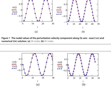
In Figure the comparison between the numerical and the exact nodal values of the velocity component along the Oxaxis is made in case of considering nodes on the boundary (a), respectively nodes (b), andε= ..
In Figures and the comparisons between the nodal values of the component along theOyaxis, and between the nodal values of the local pressure coefficient are performed, for the same values of the mentioned parameters.
Good agreement between the exact and the numerical solutions can be observed, even if we have consideredε= ., and only , respectively , boundary elements for the boundary discretization.
Figure 1 The nodal values of the perturbation velocity component alongOxaxis - exact (vx) and
numerical (Ux) solution. (a)30 nodes;(b)45 nodes.
Figure 2 The nodal values of the perturbation velocity component alongOyaxis - exact (vy) and
Figure 3 The nodal values of the local pressure coefficient - exact (cp) and numerical (Cp) solution. (a)30 nodes;(b)45 nodes.
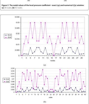
Figure 4 The errors between the numerical and the exact nodal values of the perturbation velocity
component alongOxaxis - modified shape functions (ErrX), truncation method (ErtX). (a)30 nodes;
(b)45 nodes.
Figure 5 The errors between the numerical and the exact nodal values of the perturbation velocity
component alongOyaxis - modified shape functions (ErrY), truncation method (ErtY). (a)30 nodes;
(b)45 nodes.
method. Because the numerical values are very close to the exact one in both cases the comparison is made through the absolute errors that appear.
ErrX,ErrY denote the absolute errors between the numerical and the exact values of the velocity components alongOx, respectivelyOy, when the numerical ones are got with the developed method, so using modified shape functions, and analogous notations,ErtX,
ErtY, are used when the numerical solutions are obtained using the truncation method. In Figure comparisons betweenErrXandErtXare made for the case of nodes on the boundary (a), respectively for nodes (b), andε= ..
In Figure similar comparisons are made forErrYandErtY.
From these graphics we can see that using modified shape functions for the treatment of singularities leads to better numerical results, the errors being much lower in this case. The coefficients arising from integrals with singular kernels greatly influence the well behavior of the system the problem is reduced at, and that is why it is very important to choose a suitable technique to evaluate them with great accuracy.
get a good accuracy for the numerical solution in both situations but, when using modi-fied shape functions, the numerical solution was improved, even for the small numbers of boundary elements , respectively , and forε= ..
Implementing an efficient method to evaluate the integrals of singular kernels can lead to numerical solutions of great accuracy, and this paper recommends the techniques based on modified shape functions as useful tools to succeed in this.
Competing interests
The author declares that she has no competing interests.
Acknowledgements
The author is very grateful to the reviewers for their valuable suggestions and useful comments, and thus for their help in the improvement of the original manuscript.
Received: 2 November 2014 Accepted: 23 January 2015
References
1. Banerjee, PK, Mukherjee, S: Developments in Boundary Element Methods, vol. 3. Elsevier, London (1984) 2. Banerjee, PK, Watson, JO: Developments in Boundary Element Methods, vol. 4. Elsevier, London (1986) 3. Bonne, M: Boundary Integral Equation Methods for Solids and Fluids. Wiley, New York (1995)
4. Brebbia, CA, Telles, JCF, Wobel, LC: Boundary Element Theory and Application in Engineering. Springer, Berlin (1984) 5. Brebbia, CA, Walker, S: Boundary Element Techniques in Engineering. Butterworth, London (1980)
6. Carabineanu, A: The study of the potential flow past a submerged hydrofoil by the complex boundary element method. Eng. Anal. Bound. Elem.39, 23-35 (2014)
7. Ferziger, JH, Peric, M: Computational Methods for Fluid Dynamics, 2nd rev. edn. Springer, Berlin (1999)
8. Carabineanu, A: A boundary element approach to the 2D potential flow problem around airfoils with cusped trailing edge. Comput. Methods Appl. Mech. Eng.129, 213-219 (1996)
9. Carabineanu, A: A boundary integral equations approach for the study of the subsonic compressible flow past a cusped airfoil. Nonlinear Anal.30(6), 3449-3454 (1997)
10. Drago¸s, L, Dinu, A: Application of the boundary element method to the thin airfoil theory. AIAA J.28, 1822-1824 (1990)
11. Drago¸s, L: Mathematical Methods in Aerodinamics. Romanian Academy Publishing, Bucure¸sti (2000)
12. Drago¸s, L, Dinu, A: A direct boundary integral method for the two-dimensional lifting flow. Arch. Mech.47, 813 (1995) 13. Katz, J, Plotkin, A: Low Speed Aerodynamics. Cambridge University Press, Cambridge (2001)
14. Grecu, L: A solution with cubic boundary elements for the compressible fluid flow around obstacles. Bound. Value Probl.2013, 78 (2013). doi:10.1186/1687-2770-2013-78
15. Marin, M: Some estimates on vibrations in thermoelasticity of dipolar bodies. J. Vib. Control16(1), 33-47 (2010) 16. Marin, M, Florea, O: On temporal behaviour of solutions in thermoelasticity of porous micropolar bodies. An. ¸Stiin¸t.
Univ. ‘Ovidius’ Constan¸ta, Ser. Mat.22(1), 169-188 (2014)
17. Marin, M, Stan, G: Weak solutions in elasticity of dipolar bodies with stretch. Carpath. J. Math.29(1), 33-40 (2013) 18. Grecu, L: A solution of the boundary integral equation of the theory of infinite span airfoil in subsonic flow with linear
boundary elements. Ann. Univ. Buchar. Math. Ser.LII(2), 181-188 (2003)
19. Grecu, L, Demian, G, Demian, M: Different kinds of boundary elements for solving the problem of the compressible fluid flow around bodies - a comparison study. In: Proceedings of the World Congress on Engineering, London. Lecture Notes in Engineering and Computer Science, vol. II, pp. 972-977 (2008)
20. Vladimirescu, I, Grecu, L: Weakening the singularities when applying the BEM for 2D compressible fluid flow. In: Proceedings of the International Multi-Conference of Engineers and Computer Scientists, Hong Kong. Lecture Notes in Engineering and Computer Science, pp. 2224-2229 (2010)