A SIMD ENVIRONMENT FOR GENETIC ALGORITHMS WITH INTERCONNECTED SUBPOPULATIONS
DEVARAYA PRABHU∗ AND BILL P. BUCKLES† AND FREDERICK E. PETRY†
Abstract. The algorithmic form of GAs conforms well to SIMD computing environments with relatively minor adjustments to the operators. In this paper we consider in detail a GA implementation on a MasPar machine. The question of the degree to which control parameters affecting intercommunication impact performance is addressed using ANOVA methods. The purpose is to supplant anecdotal experience with statistical evidence. A set of control parameters—topology, migration operator, migra-tion radius, and migramigra-tion probability—were chosen together with four representative levels of each. Metrics for three response variables—efficiency, diversity, and schema propagation—were developed that allowed insight into the behavior under the various parametric conditions. These were incorporated into three 4×4×4×4 randomized factorial experiment designs. Among other things, it was determined that the interconnection topology is not in itself a significant factor but the extent of connectivity and frequency of communication are. An important outcome of this study is that, while the individual factors are significant, the factors do not interact in unexpected ways.
Key words. Genetic algorithms, massively parallel computation, communicating subpopulations, migration, Royal Road functions, experiment design.
1. Introduction. Because of the complexity of large optimization problems, the value of parallel realiza-tions of optimization algorithms has become quite evident [10, 11]. In particular, in this paper we present a study of an approach to parallel genetic algorithms.
Amenability to parallelization has always been viewed as a major strength of Genetic Algorithms (GAs). GAs operate on populations of individuals. When the population is distributed into (perhaps overlapping) subpopulations, the introduction of new operators is possible as well as altering the semantics of existing ones. We consider a GA to be parallel if its operators reflect the new interactions that are enabled by the presence of subpopulations.
Furthermore, we are interested in the case for which there are thousands, not dozens, of subpopulations. When there are a massive number of subpopulations, there are larger number of local behaviors competing for the opportunity to expand and their expansion is more acutely observable. The operators that affect subpopulation interactions are defined in part by parameters. In some cases, the number of alternative values for these parameters increase as the number of subpopulations increase. Thus choices made by algorithm designers must be more informed. These two factors, measurability of effects and the need for insights, make massively parallel GAs a useful domain of investigation.
One aspect of this paper is the methodology that is applied, namely, experimental design methods [21, 29]. It has the purpose of establishing the quantitative significance of various factors, singly and in combination, that affect performance. This is in contrast to the “typical” GA experiment that quantifies performance prediction but only qualifies the factors affecting the prediction. The method used here, we believe, should be used more often because, beyond quantification, it is able to elicit evidence of the effects of factor interaction. That is, how the effect of factors change when used in combination with others.
The SIMD parallel genetic algorithm is analyzed. Its structure tends to be uniform across many applica-tions and platforms thus identification of factors to investigate requires less subjective judgment. Many SIMD computers are in use and the architecture itself is now re-emerging in the context of special-purpose VLSI plug-ins.
Using experiment design methods tends to require many individual trials over a small number of factors. In this case, more than 2,500 individual instances of the algorithm comprised the single experiment reported. The outcome showed all factors investigated – network topology, migration policy, migration probability, and migration radius—were significant at confidence levels ranging from 90% to 99%. A key question was: Do these factors interact with each other in a simple additive fashion or in a more complex manner? It was found that the interactive effects were sufficiently close to additive that no special precautions by the practitioner are necessary.
∗i2Technologies, 1603 LBJ Freeway, Suite 780, Dallas TX 75234
†The Center for Intelligent and Knowledge-based Systems, Department of Electrical Engineering & Computer Science, Tulane University, New Orleans, LA 70118. Dev [email protected] {buckles, petry}@eecs.tulane.edu
2. Background.
2.1. Sequential GAs. Genetic algorithms originated from the studies of cellular automata, conducted by John Holland [22]. A GA is a search procedure modeled on the mechanics of natural selection rather than a simulated reasoning process. Domain knowledge is embedded in the abstract representation of a candidate solution termed an organism. Organisms are grouped into sets called populations. Successive populations are called generations. A generation GA creates an initial generation,G(0), and for each generation,G(t), generates a new one,G(t + 1). An abstract view of the algorithm is
generate initial population, G(0)
evaluateG(0) t:= 0
repeat
t:=t+ 1
generate G(t)using G(t−1)
evaluateG(t)
until solution is found.
The operation “evaluateG(t)” refers to the assignment of a figure of merit to each of the population’s organisms. In simple GAs, an alternative exists to replacing an entire population at once; that alternative is to replace one organism in the population whenever a new organism is created. This variant is known as a steady state GA.
In most applications, an organism consists of a single chromosome. A chromosome of length nis a vector of the formhx1, x2, . . . , xni. where each xi is an allele, or gene. The domain of values from which xi is chosen is
called the alphabet of the problem. Frequently, the alphabet used consists of the binary digits{0, 1}. We can view a specific chromosome as representative of many patterns. Using # as “don’t care,” an example pattern or schema over the binary alphabet ish##110#i. The chromosomesh111100iandh101100iare specific instances of this and other schemata; for example, h##100i. The order of a schema is the number of non-# symbols it contains. Its length is the distance from the first to the last non-# position. Thus, the length ofh#1#0#1iis four, and its order is three.
GAs differ from traditional search techniques in several ways
• First, GAs optimize the trade-off between exploring new points in the search space and exploiting the information discovered thus far. This was proven using an analogy with the k-armed bandit (an extension of the one-armed bandit) problem.
• Second, GAs have the property of implicit parallelism. Implicit parallelism means that the GA’s effect is equivalent to an extensive search of hyperplanes of the given space, without directly testing all hyperplane values. Each schema denotes a hyperplane.
• Third, GAs are randomized algorithms, in that they use operators whose results are governed by probability. The results for such operations are based on the value of a random number.
• Fourth, GAs operate on several solutions simultaneously, gathering information from current search points to direct subsequent search. Their ability to maintain multiple solutions concurrently makes GAs less susceptible to the problems of local maxima and noise.
As noted, GAs are randomized—but not random—search algorithms. Each organism represents a point (that is, an intersection of hyperplanes) in the search space. Randomization must balance two competing concerns, exploration and exploitation. A solution cannot be tested unless it appears as an organism. Therefore, a reasonable number of solutions must be explored. On the other hand, unlimited exploration would not be efficient search. The strength of highly fit organisms must be exploited and allowed to propagate in the population. Yet, giving too much precedence to such organisms results in premature termination at a local optimum.
We can compare GA recombination operators to controlled breeding among, say, thoroughbred horses. The objective is to combine highly fit organisms to produce a still more fit individual. Both the selection of “parents” and the steps within the recombination operators are randomized. Parent selection dynamics are based on an application-dependent measure of an organism known as the fitness function, fi (fi is a figure of
in the strength of GAs. The greater the fitness value of an organism, the more likely that the organism will be selected for recombination.
There are two popular approaches for implementing selection. The first, roulette selection, assigns a prob-ability to each organism,i, computed as the proportion
Fi=fi/
X
j
fj
A parent is then randomly selected, based on this probability. A second method, deterministic sampling, assigns to each organism,i, a value
Ci =RN D(Fi×n) + 1
wherenorganisms reside in the population (RN Dmeans round to integer). The selection operator then assures that each organism participates as a parent exactlyCi times.
Parents participate in the later recombination operations. Alleles from the parents are mixed via an operator called a crossover rule, of which many exist. Simple one-point crossover of chromosomes from two parents at a random point,j, is illustrated by
hxi x2 · · ·xj xj+i xj+2· · ·xni (2.1)
+ (2.2)
hy1y2 · · ·yj yj+1 yj+2· · ·yni (2.3)
= (2.4)
hx1 x2 · · ·yj yj+1 yj+2· · ·yni (2.5)
where the result is a chromosome of the offspring and is placed in the next generation.
A mutation is the random change of an allele from one alphabet value to another. For a problem over the binary alphabet, the original allele is exchanged for its complement. The mutation operator offers the opportunity for new genetic material to be introduced into a population. From the theoretical perspective, it assures that—given any population—the entire search space is connected. The new genetic material does not originate from the parents and is not introduced into the child by crossover. Rather, it occurs after crossover a small percentage of the time.
Several stopping criteria exist for the algorithm. The algorithm may be halted when all organisms in a generation are identical, whenfi =fj for alli andj, or when|fi−fj|< T OLfor some small valueT OLand
alliand j. An alternative criterion would halt after a fixed number of evaluations and take the best solution found.
2.2. Parallel GAs. Parallel versions of GAs have, more often than not, different semantics from the canonical serial algorithm [6, 45]. In other words, the behavior of the algorithm in terms of the computational actions taken as well as the the results generated for any given set of inputs can be expected to differ for the two versions. In contrast, for most other algorithms, parallelization usually implies a parallel version of the algorithm which maintains the semantics of the serial version. Not surprisingly, early parallel GA implementations (e.g. [34]) focused mainly on achieving computational speedup. There have been a variety of applications of parallel GAs including topics such as fuzzy logic controller design [1], VLSI routing [25], financial market computations [32], SAT methods [15], land use modeling [49], and many others [2].
The interaction among the demes can take two forms: migration andoverlapping selection [7]. Migration refers to the process of periodic import of population members from neighboring demes into the local subpopu-lation. In the artificial setting of parallel GAs, this involves a sequence of export-import-replace actions. First, every deme must decide on candidates for export or emigration from the local subpopulation, which in turn can be imported by the neighboring demes. Next, a deme can decide to import or immigrate some of such can-didate emigrants available in the neighboring demes. The frequency of import is determined by themigration probability. Since most parallel GA models enforce fixed size populations, a necessary third step would be to incorporate the newly imported members into the local subpopulation by replacing local members.
A different kind of interaction among the demes is based on the notion of selection using effectively over-lapping subpopulations. In this scheme, during the selection and reproduction stage of GAs, some of the neighboring subpopulations are also taken into consideration along with the local subpopulation. Thus, using k neighboring demes and a subpopulation size of n at each deme, selection and reproduction step results in samplingnmembers from the pool of size (k+ 1)×n. Depending on such overlap, the effective subpopulations employed over all the demes constitute either a partition or a covering set of the global population. Obviously, a meaningful migration operation in such a model can be designed only by considering the demes which are not in the same selection pool.
2.3. Related Research. Here we focus on parallel GAs that support the deme concept. It was recognized early that a variety of choices existed with respect to the spatial distribution of population members [41, 5]. At one end of the spectrum are so-called coarse-grained parallel GAs [3]. In this case, the global population is divided into a few distinct non-overlapping subpopulations. Communication among them is accomplished by periodic migration [12, 13]. Selection within a subpopulation is an issue but there are no inter-deme selec-tion issues. If a parallel computer is applied to coarse-grained GA simulaselec-tion, a MIMD architecture is most appropriate [43].
Rigorous experimentation with coarse-grained GAs was first performed by Tanese [44]. She examined the frequency and subpopulation fraction for migration. It was discovered that moderate values of each are the most effective. She also noted something else that was peculiar: Even in the absence of any inter-deme communication, the parallel GA with small subpopulations performed better than the serial GA. Forrestet al., in follow-up work [17], determined that this was an artifact of the problem to which the GA was applied (a subset of Walsh functions). The coarse-grained approach allows considerable freedom such as varying control parameters, e.g., crossover rate, between subpopulations [44], varying the representation from one subpopulation to the next [37], and even dynamically varying the subpopulation sizes and number of subpopulations [46, 20]. In contrast, a fine-grained parallel GA is, strictly speaking, one in which the number of demes is the same as the population size. That is, each deme consists of one individual. A classic example is one reported by Manderick et al. [26]. In this class of GAs the principal issue is selection policy (radius, for example) [14]. A SIMD architecture is the more appropriate parallel computer for fine-grained GA simulations. Some other terms that have been used for grained GAs include cellular GAs [47] and diffusion GAs [33]. The fine-grained approach has also been applied to evolution strategies to study different selection schemes [18]. Cellular programming of cellular automata is an approach that is also related to fine-grained parallel GAs [40, 9].
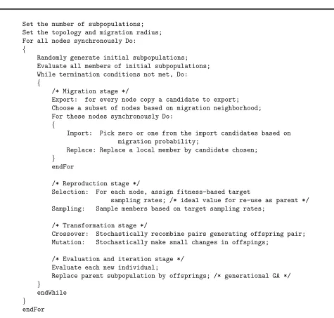
M¨uhlenbein initially developed a fine-grained GA [30] on a double-ring grid that incorporated hill-climbing. Later, the system was extended [31] in a manner that incorporated non-singleton subpopulations with both inter-deme selection and migration issues and so was not strictly fine-grained. The algorithm we have used is also not strictly fine-grained, but tends in that direction [35]. Small subpopulations were isolated with respect to selection but connected with respect to migration. This was in accordance with the controlled variables we wished to study. Otherwise, the algorithm as illustrated in Figure 2.1 has all the recognizable elements of a serial GA.
Set the number of subpopulations; Set the topology and migration radius; For all nodes synchronously Do:
{
Randomly generate initial subpopulations; Evaluate all members of initial subpopulations; While termination conditions not met, Do: {
/* Migration stage */
Export: for every node copy a candidate to export; Choose a subset of nodes based on migration neighborhood; For these nodes synchronously Do:
{
Import: Pick zero or one from the import candidates based on migration probability;
Replace: Replace a local member by candidate chosen; }
endFor
/* Reproduction stage */
Selection: For each node, assign fitness-based target
sampling rates; /* ideal value for re-use as parent */ Sampling: Sample members based on target sampling rates;
/* Transformation stage */
Crossover: Stochastically recombine pairs generating offspring pair; Mutation: Stochastically make small changes in offspings;
/* Evaluation and iteration stage */ Evaluate each new individual;
Replace parent subpopulation by offsprings; /* generational GA */ }
endWhile }
endFor
Fig. 2.1. The parallel genetic algorithm
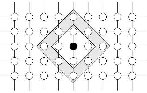
neighborhood consists of any other strongly connected subgraph of the topology. Figure 3.2 shows an example of compact neighborhoods forr= 1 and r= 2 for a node in a 4-neighbor torus topology.
Selection using overlapping subpopulations—a form of subpopulation interaction—is based on the notion of compact neighborhoods. We define theselection neighborhoodof size rs, termedselection radius, for a node
to be the corresponding compact neighborhood of that node. LetKS denote the set of subpopulations in the
neighborhood. By extending the chances of reproduction in the local node to members of all the subpopulations in the selection neighborhood, overlapping subpopulations can be effectively simulated based on the selection neighborhood. We consider only the cases for whichrs = 0, that is, the selection neighborhood is the local
subpopulation.
Subpopulation interaction by migration provides access to members of subpopulations that lie outside the selection neighborhood. Given a selection radius ofrs, we define themigration neighborhoodof sizermto be the
Fig. 3.1.Subpopulations in ring, tree, 4- and 8-neighbor torus topologies. Open-ended arrows denote wrap-around connectivity.
Fig. 3.2. Compact neighborhoods for a node of a four-torus topology. The nodes in the inner shaded area are included for r= 1. The nodes in both the shaded areas are included forr= 2.
subpopulations for the size (rs+rm), then the set of subpopulations available for the migration operation is
defined by (KS+M −KS). Figure 3.3 illustrates a migration neighborhood for rs = 1 and rm = 1. For a
zero-valued selection radius, the migration neighborhood reduces to the compact neighborhood of sizerm, sans
the reference node.
4. Experimental Design. Many empirical studies reported in the computer literature compare one method with another or the effect of one factor. This is in contrast to the natural sciences in which it is common to simultaneously study the effects of a number of factors and their interactions. The study here is closer in spirit to the principles of statistical experiment design as first used in agricultural, and then manufac-turing, settings. At least one previous study [39] of GAs has adopted a similar strategy.
Specifically, we employed an (m1×m2×m3×m4)−factorial design with complete randomization of trials.
That is to say, there were fourfactors(independent variables) withm1, m2, m3,andm4levels, respectively. A
levelis a quantitative or qualitative value at which a factor is tested. An experimentconsists of a set of trials. Atrialis a test involving each factor set at one of its levels. (In this experiment, a trial consists of one complete run.) Each trial corresponds to a single measurement of a response variable (dependent variable). Trials at the same factor levels are repeated several times with different initial conditions in order to obtain meaningful statistical properties.
Fig. 3.3.Migration neighborhood for a node in four-torus topology, givenrs= 1. The nodes in the shaded area are included by a migration radius ofrm= 1.
conditions as is needed in studies such as this. The Royal Road functions were designed to reward the discovery of lowest level building blocks of the optimal solution as well as the successful recombination of such blocks into higher level blocks in a hierarchical fashion. Royal Road functions have been widely used in a number of areas, for example, crossover variations [42], dual GAs [50] and applications such as learning of neural networks [23].
Here we briefly describe the function adopting the symbols and terminology used by Holland [28] and Jones [24]. For this problem, populations are formed from individuals over the binary alphabet. The structure of the solutions in the population is uniformly specified by the triplehb, g, ki. Each genome is composed of 2k
basic blocks of length (b+g). Thus, each individual consisted of 240 genes using the parameter values shown in Table 4.1. Within each block, allele values at pre-specified b positions (block bits) are relevant for fitness computation and the allele values of the remainingg positions (gap bits) do not affect the fitness. Such basic blocks are called level-0 blocks. A level-0 block is considered complete when all of its block bits take the value 1. Even-odd pairs of level-0 blocks comprise level-1 blocks. Level-iblocks, for 1≤i≤k, are comprised of even-odd pairs of level-(i-1) blocks. Further, any level-iblock is considered complete if the two adjacent blocks forming its constituent level-(i-1) even-odd pair are both complete.
The computation of the Royal Road function used itself can be described in two parts, typically referred to as thepart and thebonus computations. partcomputes a value with respect to level-0 blocks using two parameters,m∗and v. Letj stand for the number of 1s present in thebblock bits for a given level-0 block in the genome. Now, thepartcontribution for that block is given by (j×v), ifj≤m∗, and by ((m∗−j)× −v), ifm∗< j < b. The contribution is zero (0) ifj=b. The fullpartvalue is computed by summation over all the level-0 blocks. The intentional penalties for near-optimal blocks at the lowest level make this problem harder for hill-climbing algorithms.
Thebonuscomputation rewards the presence of complete blocks at each leveli, 0≤i≤k, and is specified by the parametersu∗ andu. Recall that only the presence of a corresponding even-odd pair of complete blocks of level-(i-1) can generate a complete block at level-i. Letjstand for the number complete blocks present in the genome for a given level-i. Thebonuscontribution for level-iis zero, ifj= 0 and is given by (u∗+ (j−1)×u) forj >0. The completebonusvalue for the genome is computed by summation over all the levels. The fitness function itself is again a sum ofpartandbonus values. The parameter values used in this study are shown in Table 4.1 and they are similar to the values suggested by Holland.
Table 4.1
Parameters for the Royal Road function.
Parameters Value
k 4
b 8
g 7
m∗ 4
v 0.02
u∗ 1.0
u 0.3
Table 4.2 Experimental Factors
Factor Symbol Levels
Topology G {G0 = Ring,G1 = Tree,
G2 = 4-Torus,G 3 = 8-Torus} Migration Radius R {R 0 = 1,R 1 = 3,R 2 = 5,R 3 = 7} Migration Operator O {O 0 = Import-random & Replace-random,
O 1 = Import-random & Replace-worst, O 2 = Import-best & Replace-random, O 3 = Import-best & Replace-worst}
Migration Probability P {P 0 = 0.0,P 1 = 0.33,P 2 = 0.66,P 3 = 1.0}
available. The experiments were performed on the MasPar MP-216 at NASA/GSFC using MPGA [36], a massively parallel GA package developed by the authors.
4.2. Response Variables. The effect of the factors was tested using response variables corresponding to population diversity, schemata propagation, and search efficiency. More than one method was employed [35], but here we restrict the discussion to one representative method for each.
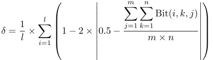
An objective in a GA, parallel or serial, is to obtain a balance between population diversity and the speed of convergence,i. e.,exploration and exploitation. Therefore studying the effect of the factors on the population diversity is important. To measure diversity we use a metric similar in spirit to the one described by Collins [13, pages 118–120].
δ= 1 l ×
l
X
i=1
1−2×
0.5−
m
X
j=1 n
X
k=1
Bit(i, k, j)
m×n
(4.1)
where, l is the length of the chromosome in bits, m is the number of subpopulations, andn is the number of chromosomes in each subpopulation. Bit(i, k, j) denotes the value of theith bit of the kth member in thejth subpopulation. δ is in the range [0,1] where zero (0) is the response for a global population consisting of one individual replicated and one (1) is the response when the global population is maximally diverse,i. e.,at each position all alleles are uniformly distributed.
Schemata propagation is used here to mean the extent to which a fit schema is present among all the subpopulations. A priori choice of a single schema to be monitored is not practical because there are a number of search paths from different schemata that lead to an optimum. Taking advantage of the problem symmetry, eight complementary schemata were chosen for monitoring. These schemata are shown in Figure 4.1. At selected generations the subpopulations were examined for presence of the schemata. In the results of Section 5 the final measurement is used.
GA parameters used in the experiment.
Parameters Value
Number of subpopulations 16,384
Subpopulation size 10
Number of maximum generations 100
Export operator Export-current-best
Selection radius 0
Selection operator Ranking
Elitism No
Sampling operator Stochastic universal sampling
Mutation operator Bit-mutation
Mutation probability 0.005 per bit
Crossover operator Two-point crossover
Crossover probability 0.7
having no neighbors (with respect to the topology) also containing instance(s). That is, only those subpopula-tions in which the schema could plausibly have occurred as a result of migration are counted. The maximum for the eight candidate schemata was chosen as the basis for the response. This accounts for the various search paths the GA might traverse. The response variable was normalized to be the fraction of the number of applicable subpopulations meeting the propagation criteria.
1 1· · ·1 #· · ·# #· · ·# #· · ·# #· · ·# #· · ·# #· · ·# #· · ·# 2 #· · ·# 1· · ·1 #· · ·# #· · ·# #· · ·# #· · ·# #· · ·# #· · ·# 3 #· · ·# #· · ·# 1· · ·1 #· · ·# #· · ·# #· · ·# #· · ·# #· · ·# 4 #· · ·# #· · ·# #· · ·# 1· · ·1 #· · ·# #· · ·# #· · ·# #· · ·# 5 #· · ·# #· · ·# #· · ·# #· · ·# 1· · ·1 #· · ·# #· · ·# #· · ·# 6 #· · ·# #· · ·# #· · ·# #· · ·# #· · ·# 1· · ·1 #· · ·# #· · ·# 7 #· · ·# #· · ·# #· · ·# #· · ·# #· · ·# #· · ·# 1· · ·1 #· · ·# 8 #· · ·# #· · ·# #· · ·# #· · ·# #· · ·# #· · ·# #· · ·# 1· · ·1
Legend: 1· · ·1 ⇒11111111#######11111111####### #· · ·# ⇒##############################
Fig. 4.1.The list of schemata monitored.
Finally, search efficiency is measured in terms of the time taken to reach the optimum. In this case, the number of generations taken to find the globally optimal solution is recorded. If a particular trial failed to locate the optimum, the preset value of maximum number of generations was used. Typically, the value for efficiency tends to be domain-specific. However, it is hoped that the premise underlying the design of the Royal Road functions—building-block hypothesis—renders the results a significance sufficiently independent of specific applications.
performance. A factor may affect performance by itself, in combination with other factors, or both. The most important result here, given that each factor investigated affected performance as might be expected, is that there were no unusual effects that occurred when factors were used in combination. That is, the effects in combination are a linear combination of the effects of each single factor.
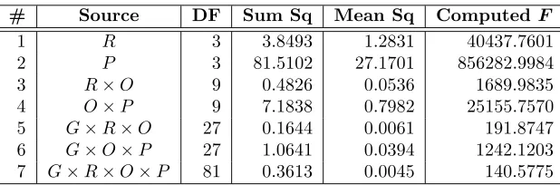
5.1. ANOVA. An illustrative ANOVA is shown in Table 5.1. A complete table for each response variable is in the appendix. The source column lists the factor (e.g., R or migration radius) or factor combination (e.g.,O×P or migration operator with migration probability) that was tested for its effects. The last column (Computed F) is a statistic that is compared to standard tables to extract the degree of confidence that the source factor or source combination has a significant influence on the response. Further description of the ANOVA tables and the columns can be found in the appendix.
Table 5.1
Abbreviated ANOVA for global allelic diversity
# Source DF Sum Sq Mean Sq ComputedF
1 R 3 3.8493 1.2831 40437.7601
2 P 3 81.5102 27.1701 856282.9984
3 R×O 9 0.4826 0.0536 1689.9835
4 O×P 9 7.1838 0.7982 25155.7570
5 G×R×O 27 0.1644 0.0061 191.8747
6 G×O×P 27 1.0641 0.0394 1242.1203
7 G×R×O×P 81 0.3613 0.0045 140.5775
Since a large computedF-statistic value relative to the corresponding critical value indicates that the effect under scrutiny is significant under normal circumstances, the ANOVA tables shown would lead one to conclude that all the factors and their interactions have significant effect on the response variables. This is, in fact, conclusive with respect to the single factor rows in Table 5.1 and the tables in the appendix. However, it is not conclusive with respect to the factor interaction effects. Their appearance of significance may be a carry-over effect of the individual factor effects. The standard recourse in such instances is to scrutinize in greater detail the effects. Generally, a graphical approach is used and that approach is taken in the following sections. For completeness, we examine the individual factors this way as well as the factor interactions.
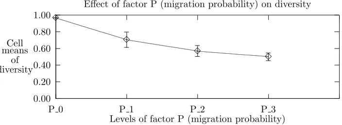
5.2. Effects of individual factors. Note that in the ANOVA analysis, Tables A.1, A.2, and A.3, the computed F-statistic values for migration probability factor are the greatest. Migration probability, in fact, clearly affects all three responses as is evident from Figure 5.1. In the single factor graphs, the feature one looks for in order to confirm visually that a factor affects performance is a curve with a slope other than zero. The response values (Y-axis) for these and succeeding plots are described in Section 4.2. To summarize, theY-axis of the top graph of Figures 5.1-5.4 is the value from Eq. 4.1. TheY-axis of the middle graph of the figures is the fraction of subpopulations in which a key schema occurs (plausibly) by means of migration. Finally, the Y-axis of the bottom graph is the number of generations required for convergence. For single-factor plots, each data point is an average over all possible combinations of other factors, i. e., each point is an average of 640 values. The error bars depict the standard deviation.
Figure 5.1 emphatically demonstrates that subpopulations when interconnected behave differently than when isolated, i. e., P = 0. Further, up to a point, the level of intercommunication, as reflected by the magnitude of migration probability, makes a difference. In the absence of migration, i. e., zero probability, there is little exploitation (i. e., maximal diversity), schema proliferation only by chance rediscovery, and poor search efficiency. In contrast, moderate to high migration probabilities result in significantly different behavior with respect to all response variables. As is seen in the following subsections, migration probability also exhibits significant interaction with other factors.
0.00 0.20 0.40 0.60 0.80 1.00
P 0 P 1 P 2 P 3
Cell means
of diversity
Levels of factor P (migration probability) Effect of factor P (migration probability) on diversity
3
3
3 3
0.00 0.20 0.40 0.60 0.80 1.00
P 0 P 1 P 2 P 3
Cell means
of schema
prop.
Levels of factor P (migration probability)
Effect of factor P (migration probability) on schemata propagation
3
3
3 3
0 20 40 60 80 100
P 0 P 1 P 2 P 3
Cell means
of gens
to optimum
Levels of factor P (migration probability)
Effect of factor P (migration probability) on search efficiency
3
3
3
3
Fig. 5.1. Effect of factor P (Migration Probability) on the response variables
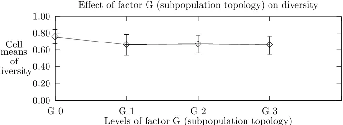
Figures 5.3 and 5.4 indicate that the independent effects of topology and migration radius are minimal. The changes in responses between the first and the second data points of each plot might best be explained in terms of changes in the degree of connectivity. The similarity among the remaining data points suggest that further increases in the degree of connectivity have little effect.
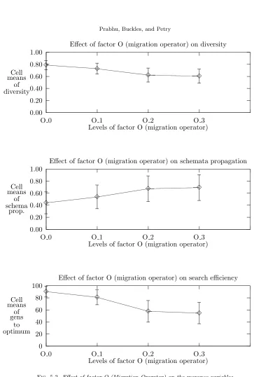
5.3. Effects of multiple factor interactions. One method for examining in more detail the higher order interactions is to visually compare different components of the effect under scrutiny, using two factors at a time. The cell means of the response variable are plotted against one of the factors, for each level of the second factor. All the cell means are averaged over all the combinations of levels of the remaining factors.
0.00 0.20 0.40 0.60 0.80 1.00
O 0 O 1 O 2 O 3
Cell means
of diversity
Levels of factor O (migration operator) Effect of factor O (migration operator) on diversity
3 3
3 3
0.00 0.20 0.40 0.60 0.80 1.00
O 0 O 1 O 2 O 3
Cell means
of schema
prop.
Levels of factor O (migration operator)
Effect of factor O (migration operator) on schemata propagation
3 3
3 3
0 20 40 60 80 100
O 0 O 1 O 2 O 3
Cell means
of gens
to optimum
Levels of factor O (migration operator)
Effect of factor O (migration operator) on search efficiency
3
3
3 3
Fig. 5.2.Effect of factor O (Migration Operator) on the response variables
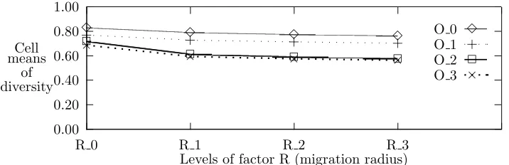
additive (linear) combination of the individual factor levels. The visual feature one looks for to “not reject the null hypothesis” is roughly parallel lines. The four plots in Figure 5.5 are roughly parallel to each other, thus the interaction effect is not significant with respect to diversity. Figure 5.6 shows an example that might suggest some factor interaction but the lines are parallel statistically speaking.
When we consider any three-factor interaction, one should examine all the plots that can be generated by choosing two factors at a time for each level of the third factor. For any response variable there are twelve graphs for each of the four possible three-factor interactions. If most of those graphs show parallel plots, we can conclude the effect of the interaction is insignificant. A similar procedure can be carried out to determine the significance of the four-factor interaction.
0.00 0.20 0.40 0.60 0.80 1.00
G 0 G 1 G 2 G 3
Cell means
of diversity
Levels of factor G (subpopulation topology) Effect of factor G (subpopulation topology) on diversity
3
3 3 3
0.00 0.20 0.40 0.60 0.80 1.00
G 0 G 1 G 2 G 3
Cell means
of schema
prop.
Levels of factor G (subpopulation topology)
Effect of factor G (subpopulation topology) on schemata propagation
3
3 3 3
0 20 40 60 80 100
G 0 G 1 G 2 G 3
Cell means
of gens
to optimum
Levels of factor G (subpopulation topology)
Effect of factor G (subpopulation topology) on search efficiency
3
3 3
3
Fig. 5.3.Effect of factor G (Subpopulation Topology) on the response variables
Since the migration probability and migration operator have the greatest single factor effects, as can be expected, they exhibit the most pronounced second-order effects. The second order effect ofO×P on diversity is shown in Figure 5.6. Similar behavior can be observed with respect to the other response variables. In Figure 5.6, there is evidence explaining the interaction of O ×P. Namely, the import policy impacts the migration effect to a greater extent than the replacement policy. Also, reinforcing our expectations, a migration probability of zero produces the most distinctively different results.
0.00 0.20 0.40 0.60 0.80 1.00
R 0 R 1 R 2 R 3
Cell means
of diversity
Levels of factor R (migration radius) Effect of factor R (migration radius) on diversity
3
3 3 3
0.00 0.20 0.40 0.60 0.80 1.00
R 0 R 1 R 2 R 3
Cell means
of schema
prop.
Levels of factor R (migration radius)
Effect of factor R (migration radius) on schemata propagation
3 3
3 3
0 20 40 60 80 100
R 0 R 1 R 2 R 3
Cell means
of gens
to optimum
Levels of factor R (migration radius)
Effect of factor R (migration radius) on search efficiency
3
3 3 3
Fig. 5.4.Effect of factor R (Migration Radius) on the response variables
0.00 0.20 0.40 0.60 0.80 1.00
R 0 R 1 R 2 R 3
Cell means
of diversity
Levels of factor R (migration radius)
O 0 3
3 3 3
3 O 1 +
+ + +
+
O 2 2
2
2 2 2
O 3 ×
×
× × ×
0.00 0.20 0.40 0.60 0.80 1.00
O 0 O 1 O 2 O 3
Cell means
of diversity
Levels of factor O (migration operator)
P 0 3
3 3 3 3
P 1 +
+ +
+ + P 2 2
2
2
2 2 P 3 ×
×
× ×
×
Fig. 5.6. Effect of OxP interaction on diversity
This is probably a reflection of the effect migration radius has in a low-connectivity architecture. The plots in terms of other response variables indicate essentially the same behavior.
Contrast Figure 5.7 with Figure 5.8 in which the effects of the interaction among migration radius, migration operator, and migration probability on schemata propagation are shown. While theR×O×P interaction effect is not highly pronounced in the figure, it does assert itself in the second plot. This again is further corroboration of the importance of the import policy component of the migration operator.
The computedF-statistic for the fourth order interaction is low in a relative sense in each of the ANOVA Tables A.1, A.2, and A.3 shown in the appendix. This leads one to suspect that the interaction effect is minimal. Figure 5.9, which illustrates the fourth order interaction partially, supports this observation. The plots are in terms of the search efficiency response but the graphs of other response variables lead one to the same conclusion.
5.4. Global Behavior. Recall that in the experiments, the number of cells was 256 (4×4×4×4). Since we took 10 samples for each cell (using the same set of 10 random seeds across all the cells) a total of 2,560 runs were made. Of the 2,560 runs, the algorithm found the maximum royal road (RR) level of 4 in 1,316 runs, reached RR level 3 in 1, 834 runs, and reached RR level 2 in 1,920 runs. It reached the first level in all runs. (While we are speaking here of global behavior, let us remind the reader the 640 runs that it failed to climb above level 1 are the same runs for which the migration probability was zero, i. e., the subpopulations were isolated. Table 5.2 summarizes the global behavior. We suggest that the measure “Evaluations (Avg.)”
Table 5.2
Summary across experiments.
RR Level Reached in . . . That is . . .
Fuction Evaluations (Avg.)
Generations (Avg.)
1 2,560 runs 100% of runs 163,840 1.00
2 1,920 runs 75% of runs 2,723,840 16.63
3 1,834 runs 72% of runs 6,102,459 37.25
4 1,316 runs 51% of runs 7,809,790 47.67
(the number of function evaluations required to reach a specific level) is not as informative as the number of generations given that 16,384 evaluations are done in parallel. That is 16,384 evaluations occur between points at which the level noted.
0.00 0.20 0.40 0.60 0.80 1.00
R 0 R 1 R 2 R 3
Cell means
of schema
prop.
Levels of factor R (migration radius) RxO interaction for ring topology (G 0)
O 0 3
3 3
3 3
O 1 +
+
+ + +
O 2 2
2
2 2
2
O 3 ×
×
× × ×
0.00 0.20 0.40 0.60 0.80 1.00
R 0 R 1 R 2 R 3
Cell means
of schema
prop.
Levels of factor R
RxO interaction for tree topology (G 1)
O 0 3
3 3
3 3
O 1 +
+
+ + + O 2 2
2
2 2 2
O 3 ×
×
× × ×
0.00 0.20 0.40 0.60 0.80 1.00
R 0 R 1 R 2 R 3
Cell means
of schema
prop.
Levels of factor R
RxO interaction for 4-torus topology (G 2)
O 0 3
3 3 3 3
O 1 +
+ + + + O 2 2
2 2 2 2
O 3 ×
× × × ×
0.00 0.20 0.40 0.60 0.80 1.00
R 0 R 1 R 2 R 3
Cell means
of schema
prop.
Levels of factor R
RxO interaction for 8-torus topology (G 3)
O 0 3
3 3 3 3
O 1 +
+ + + + O 2 2
2 2 2 2
O 3 ×
× × × ×
Fig. 5.7. Partial effect of RxOxG interaction on schemata propagation
0.00 0.20 0.40 0.60 0.80 1.00
R 0 R 1 R 2 R 3
Cell means
of schema
prop.
Levels of factor R
RxO interaction for migration probability 0.0 (P 0)
O 0 3
3 3 3 3
O 1 +
+ + + +
O 2 2
2 2 2 2
O 3 ×
× × × ×
0.00 0.20 0.40 0.60 0.80 1.00
R 0 R 1 R 2 R 3
Cell means
of schema
prop.
Levels of factor R
RxO interaction for migration probability 0.33 (P 1)
O 0 3
3 3 3 3
O 1 +
+ +
+ + O 2 2
2
2 2 2
O 3 ×
×
× × ×
0.00 0.20 0.40 0.60 0.80 1.00
R 0 R 1 R 2 R 3
Cell means
of schema
prop.
Levels of factor R
RxO interaction for migration probability 0.66 (P 2)
O 0 3
3
3 3
3
O 1 + +
+ + +
O 2 2
2
2 2 2
O 3 ×
× ×
× ×
0.00 0.20 0.40 0.60 0.80 1.00
R 0 R 1 R 2 R 3
Cell means
of schema
prop.
Levels of factor R
RxO interaction for migration probability 1.0 (P 3)
O 0 3
3
3 3 3
O 1 +
+ + +
+
O 2 2
2 2 2 2
O 3 ×
× × × ×
Fig. 5.8.Partial effect of RxOxP interaction on schemata propagation
0 20 40 60 80 100
R 0 R 1 R 2 R 3
Cell means of gens to optimum
Levels of factor R
RxOxGxP interaction for ring topology and 1.0 migration probability
O 0 3
3 3
3
3
O 1 + +
+
+
+ O 2 2
2
2
2 2 O 3 ×
× × × × 0 20 40 60 80 100
R 0 R 1 R 2 R 3
Cell means of gens to optimum
Levels of factor R
RxOxGxP interaction for tree topology and 1.0 migration probability
O 0 3
3
3
3
3
O 1 + +
+
+ +
O 2 2
2
2 2
2
O 3 ×
× × × × 0 20 40 60 80 100
R 0 R 1 R 2 R 3
Cell means of gens to optimum
Levels of factor R
RxOxGxP interaction for 4-torus topology and 1.0 migration probability
O 0 3
3
3 3 3
O 1 + +
+ + +
O 2 2
2
2 2
2
O 3 ×
× × × × 0 20 40 60 80 100
R 0 R 1 R 2 R 3
Cell means of gens to optimum
Levels of factor R
RxOxGxP interaction for 8-torus topology and 1.0 migration probability
O 0 3
3
3 3 3
O 1 + +
+ + +
O 2 2
2
2 2 2
O 3 ×
×
× × ×
Fig. 5.9.Partial effect of RxOxGxP interaction on search efficiency.
results lend strong credence to a conclusion already largely accepted: There is a distinct behavioral difference between isolated subpopulations and those that communicate.
policy. On the other side of the ledger, the choice of topology does not seem to be an important one as long as the communication is bidirectional. The native topologies of SIMD architectures, such as a 4- or 8-torus, can be used without impacting the performance.
Acknowledgement. The authors wish to thank Dr. Janet Rice of the Tulane School of Public Health for invaluable guidance in both design of the experiment and interpretation of the results. This work was supported in part by a grant from Naval Oceanographic and Atmospheric Research Laboratory, Stennis Space Center, MS, Grant # N00014-89-J-6003, in part by the NASA High Performance Computing and Communications Program (Earth and Space Sciences Project) Grant NAG 5-2216, and in part by EPSCoR grant NSF/LEQSF-ADP-04.
REFERENCES
[1] E. Alba and C. Cotta,Evolution of complex data structures, Informatica y Automatica, 30 (1997), pp. 42–60. [2] E. Alba and J. M. Troya,A survey of parallel distributed genetic algorithms, Complexity, 4 (1999), pp. 31–52.
[3] S. L. amd W. Punch and E. Goodman,Coarse-grain parallel genetic algorithms: Categorization and new approach, in 6th IEEE Symp. On Parallel and Distributed Processing, IEEE Press, 1994, pp. 28–37.
[4] R. Belew and L. Booker, eds.,Proc. of Fourth Intern. Conf. on Genetic Algorithms, San Diego, CA, April 1991, Morgan Kaufmann.
[5] E. Cant´u-Paz, A survey of parallel genetic algorithms, Calculateurs Paralleles, Reseaux et Systems Repartis, 10 (1998), pp. 141–171.
[6] ,Efficient and Accurate Parallel Genetic Algorithms, Kluwer Academic Publishers, 2000.
[7] ,Migration policies, selection pressure, and parallel evolutionary algorithms, Journal of Heuristics, 7 (2001), pp. 311– 334.
[8] E. Cant´u-Paz and D. Goldberg,On the scalability of parallel genetic algorithms, Evolutionary Computation, 7 (1999), pp. 429–449.
[9] M. Capcarrere, M. Tomassini, A. Tettamanzi, and M. Sipper,A statistical study of a class of cellular evolutionary algorithms, Evolutionary Computation, 7 (1999), pp. 255–274.
[10] Y. Censor and S. Zenois,Parallel Optimization: Theory, Algorithms and Applications, Oxford University Press, 1998. [11] ,Parallel algorithms in optimization, in Handbook of Applied Optimization, M. Resende and P. Pardalos, eds., Oxford
University Press, 2002, pp. 544–559.
[12] J. P. Cohoon, S. U. Hedge, W. M. Martin, and D. Richards, Punctuated equilibria: a parallel genetic algorithm, in Grefenstette [19], pp. 148–154.
[13] R. J. Collins,Studies in Artificial Evolution, PhD thesis, University of California, Los Angeles, 1992.
[14] R. J. Collins and D. R. Jefferson,Selection in massively parallel genetic algorithms, in Belew and Booker [4], pp. 249–256. [15] G. Folino, C. Pizzuti, and G. Spezzano,A parallel hybrid method for SAT that couples genetic algorithms and local search,
IEEE Trans. on Evolutionary Computation, 5 (2001), pp. 323–333.
[16] S. Forrest, ed.,Proc. of Fifth Intern. Conf. on Genetic Algorithms, Urbana, IL, 1993.
[17] S. Forrest and M. Mitchell,The performance of genetic algorithms on Walsh polynomials: Some anomalous results and their explanation, in Belew and Booker [4], pp. 182–189.
[18] M. Gorges-Schleuter,An analysis of local selection in evolution strategies, in Proc. of Genetic and Evolutionary Compu-tation Conf., Morgan Kaufmann, 1999, pp. 847–854.
[19] J. J. Grefenstette, ed.,Proc. of Second Intern. Conf. on Genetic Algorithms, Lawrence Erlbaum Associates, 1987. [20] G. Harik, E. Cant´u-Paz, D. Goldberg, and R. Miller,The gambler’s ruin problem genetic algorithms and the sizing of
populations, Evolutionary Computation, 7 (1999), pp. 231–253.
[21] C. R. Hicks,Fundamental Concepts in the Design of Experiments, Holt, Rinehart and Winston, 1973.
[22] J. H. Holland,Adaptation in Natural and Artificial Systems, University of Michigan Press, Ann Arbor MI, 1975.
[23] T. Ichimura and Y. Kuriyama,Learning of Neural Networks with Parallel Hybrid GA Using a Royal Road Function,IEEE International Joint Conference on Neural Networks, 1998, ppp. 1131–1136
[24] T. Jones,A description of Holland’s Royal Road Function, Evolutionary Computation, 2 (1994), pp. 409–415.
[25] J. Lienig,A parallel genetic algorithm for performance-driven VLSI routing, IEEE Trans. On Evolutionary Computation, 1 (1997), pp. 329–339.
[26] B. Manderick and P. Spiessens,Fine-grained parallel genetic algorithms, in Schaffer [38], pp. 428–433.
[27] W. Martin, J. Lienig, and J. Cohoon,Island (migration) models, in Handbook of Evolutionary Computation, T. B¨ack, D. Fogel, and Z. Michalewicz, eds., Oxford University Press, 1997, pp. C6:5–8–15.
[28] M. Mitchell, S. Forrest, and J. Holland,The Royal Road for genetic algorithms: Fitness landscapes and GA perfor-mance, in Proc. 1st European Conf. on Artificial Life, MIT Press, 1992, pp. 245–254.
[29] D. C. Montgomery,Design and Analysis of Experiments, John Wiley & Sons, 1996.
[30] H. M¨uhlenbein,Parallel genetic algorithms, population genetics and combinatorial optimization, in Schaffer [38], pp. 416– 421.
[31] H. M¨uhlenbein, M. Schomich, and J. Born,The parallel genetic algorithm as function optimizer, Parallel Computing, 17 (1992), pp. 619–632.
[32] M. Oussaidene, B. Chopard, O. Pictet, and M. Tommassini,Parallel genetic programming and its application to trading model induction, Parallel Computing, 23 (1997), pp. 1183–1198.
[33] C. Pettey,Population structures: diffusion (cellular) models, in Handbook of Evolutionary Computation, T. B¨ack, D. Fogel, and Z. Michalewicz, eds., Oxford University Press, 1997, pp. C6:4–1–6.
[35] D. Prabhu,A study in massively parallel genetic algorithms with application to image interpretation, Tech. Rep. Tech Report 99-5, EECS Dept., Tulane University, New Orleans, 1999.
[36] D. Prabhu, B. P. Buckles, and F. E. Petry,MPGA: User’s guide, tech. rep., Department of Computer Science, Tulane University, New Orleans, 1995.
[37] W. F. Punch, R. C. Averill, E. D. Goodman, S. C. Lin, and Y. Ding, Using genetic algorithms to design laminated composite structures, IEEE Expert, (1995), pp. 42–49.
[38] J. D. Schaffer, ed.,Proc. of Third Intern. Conf. on Genetic Algorithms, Fairfax, VA, 1989, Morgan Kaufmann.
[39] J. D. Schaffer, R. A. Caruana, L. J. Eshelman, and R. Das,A study of control parameters affecting online performances of genetic algorithms for function ptimization, in Schaffer [38], pp. 51–60.
[40] M. Sipper,Evolution of Parallel Cellular Machines: The Cellular Programming Approach, Springer Verlag, 1997.
[41] J. Stender, Parallel genetic algorithms theory and applications, in Frontiers in Artificial Intelligence and Applications, J. Stender, ed., IOS Press, 1993.
[42] H. Suzuki and H. Sawai,Crossover accelerates evolution in GAs with a Royal Road function, in Proc. Genetic and Evolu-tionary Computation Conference, 2001, pp. 405–412.
[43] R. Tanese,Parallel genetic algorithms for a hypercube, in Grefenstette [19], pp. 177–183. [44] ,Distributed genetic algorithms, in Schaffer [38], pp. 434–440.
[45] M. Tomassini,Parallel and distributed evolutionary algorithms: A review, in Evolutionary Algorithms in Engineering and Computer Science, K. Miettien, M. M¨akek¨a, P. Neittaanm¨aki, and J. P´eriaux, eds., J. Wiley and Sons, 1999, pp. 113–133. [46] S. Tsutsu and Y. Fujimoto,Forking genetic algorithm with blocking and shrinking modes (fGA), in Forrest [16], pp. 206–213. [47] D. Whitley,Cellular genetic algorithms, in Forrest [16], pp. 658–666.
[48] D. Whitley, S. Rana, and R. Heckendorn,Exploiting seperability in search: The island model genetic algorithm, Journal of Computing and Information Technology, 7 (1999), pp. 33–47.
[49] S. Wong, C. Wong, and C. Tong,A parallelized genetic algorithm for the calibration of the Lowry Model, Parallel Com-puting, 27 (2001), pp. 1523–1536.
[50] S. Yang,Primal-dual genetic algorithms for Royal Road functions, in Proc. of the 15th IFAC World Congress, Barcelona, Spain, 21-26 July 2002, pp. 439–446.
Appendix A.
Analysis of Variance (ANOVA) for various experimental designs is adequately covered in numerous texts (e.g. [21, 29]). The experiment design used here is known as randomized factorial. There are four factors and four levels of each, thus 44 level combinations. For each level of each factor,g, r, o, p, the outcome of a single
repetition,k, is represented by ygropk. For this experiment,g∈ {1,2,3,4},r∈ {1,2,3,4}, ando∈ {1,2,3,4},
and p∈ {1,2,3,4}, andk∈ {1,2, . . . ,10}, yielding 10×44 individual trials. Thedegrees of freedom are (one
less) than than the number of choices possible for a component. For total trials (line 17 in Tables A.1-A.3) there are 2,559 (10×44−1) degrees of freedom. For any given factor (lines 1–4 in Tables A.1–A.3) there are
three (four levels – 1) degrees of freedom. For combinations of factors, the degrees of freedom are the product of the degrees for individual factors (i. e., nine for pairs, 27 for triples, and 81 for the combination of all four factors).
Table A.1
ANOVA for global allelic diversity
# Source DF Sum Sq Mean Sq ComputedF
1 G 3 4.2971 1.4324 45141.8887
2 R 3 3.8493 1.2831 40437.7601
3 O 3 14.6118 4.8706 153500.4667
4 P 3 81.5102 27.1701 856282.9984
5 G×R 9 0.6086 0.0676 2131.1502
6 G×O 9 0.9484 0.1054 3321.1950
7 G×P 9 1.5872 0.1764 5558.0741
8 R×O 9 0.4826 0.0536 1689.9835
9 R×P 9 1.6751 0.1861 5865.8867
10 O×P 9 7.1838 0.7982 25155.7570
11 G×R×O 27 0.1644 0.0061 191.8747
12 G×R×P 27 0.4341 0.0161 506.6511
13 G×O×P 27 1.0641 0.0394 1242.1203
14 R×O×P 27 0.8969 0.0332 1046.8983
15 G×R×O×P 81 0.3613 0.0045 140.5775
16 Errors 2304 0.0731 0.0000
ANOVA for schemata propagation
# Source DF Sum Sq Mean Sq ComputedF
1 G 3 16.6509 5.5503 25888.3304
2 R 3 8.4362 2.8121 13116.4494
3 O 3 27.5620 9.1873 42852.7267
4 P 3 340.6299 113.5433 529602.2027
5 G×R 9 2.4828 0.2759 1286.7461
6 G×O 9 0.7596 0.0844 393.6835
7 G×P 9 6.8043 0.7560 3526.3902
8 R×O 9 0.1485 0.0165 76.9467
9 R×P 9 3.6515 0.4057 1892.4426
10 O×P 9 22.7254 2.5250 11777.6365
11 G×R×O 27 0.8185 0.0303 141.4041
12 G×R×P 27 1.5875 0.0588 274.2432
13 G×O×P 27 3.7258 0.1380 643.6473
14 R×O×P 27 2.2732 0.0842 392.7038
15 G×R×O×P 81 1.7956 0.0222 103.3959
16 Errors 2304 0.4940 0.0002
17 Totals 2559 440.5459
Table A.3
ANOVA for search efficiency
# Source DF Sum Sq Mean Sq ComputedF
1 G 3 254008.7824 84669.5941 9667.5576
2 R 3 149389.6855 49796.5618 5685.7616
3 O 3 579318.1168 193106.0389 22048.8096
4 P 3 1124711.5105 374903.8368 42806.4464
5 G×R 9 7361.0035 817.8893 93.3864
6 G×O 9 46817.6848 5201.9650 593.9593
7 G×P 9 89067.4410 9896.3823 1129.9670
8 R×O 9 42775.2691 4752.8077 542.6746
9 R×P 9 50002.2004 5555.8000 634.3602
10 O×P 9 242684.8566 26964.9841 3078.8566
11 G×R×O 27 3590.1730 132.9694 15.1824
12 G×R×P 27 25966.8418 961.7349 109.8107
13 G×O×P 27 68730.3230 2545.5675 290.6524
14 R×O×P 27 41988.8262 1555.1417 177.5658
15 G×R×O×P 81 34339.4254 423.9435 48.4058
16 Errors 2304 20178.7000 8.7581
17 Totals 2559 2780930.8402
The fundamental idea in design of experiments is that if a factor has no significance, then the distribution of all responses is the same as the distribution of responses for a given level of the factor. That is, we could check the total mean against the mean for a specific factor level. Parametric comparisons in statistics more frequently employ an equivalent method: Determine if there are differences in the variances (mean squares) among factor levels. Letyg.... be the average of responses for a particular option, g, for the topology across all
other factors and repetitions. Similarly, lety...be the overall average for all (in this case, 2,560) responses. To
describe via example, the sum of squares for line 1 of Tables A.1-A.3 is
X
g
where n is the number of replications (10 in our case). The mean square is the sum of squares divided by the degrees of freedom. The total sum of squares is P
g
P
r
P
o
P
p
P
p(ygropk−(y)...)2. The “easy” way to
compute the error sum of squares is subtract the individual factor sums from the total sum.
Variances are compared by dividing the factor mean square by the error mean square (the F-statistic). Standard tabulations of critical F-statistic values can then be consulted to determine if the effect of a factor or an interaction on the given response variable is significant. ANOVA results for the response variables measuring population diversity, schemata propagation, and search efficiency are shown in Tables A.1, A.2, and A.3, respectively.