Quadratic Programming Feature Selection
Irene Rodriguez-Lujan [email protected]
Departamento de Ingenier´ıa Inform´atica and IIC Universidad Aut´onoma de Madrid
28049 Madrid, Spain
Ramon Huerta [email protected]
BioCircuits Institute
University of California, San Diego La Jolla, CA 92093-0402, USA
Charles Elkan [email protected]
Department of Computer Science and Engineering University of California, San Diego
La Jolla, CA 92093-0404, USA
Carlos Santa Cruz [email protected]
Departamento de Ingenier´ıa Inform´atica and IIC Universidad Aut´onoma de Madrid
28049 Madrid, Spain
Editor: Lyle Ungar
Abstract
Identifying a subset of features that preserves classification accuracy is a problem of growing im-portance, because of the increasing size and dimensionality of real-world data sets. We propose a new feature selection method, named Quadratic Programming Feature Selection (QPFS), that re-duces the task to a quadratic optimization problem. In order to limit the computational complexity of solving the optimization problem, QPFS uses the Nystr¨om method for approximate matrix diag-onalization. QPFS is thus capable of dealing with very large data sets, for which the use of other methods is computationally expensive. In experiments with small and medium data sets, the QPFS method leads to classification accuracy similar to that of other successful techniques. For large data sets, QPFS is superior in terms of computational efficiency.
Keywords: feature selection, quadratic programming, Nystr¨om method, large data set, high-dimensional data
1. Introduction
classifica-tion (Rodriguez et al., 2005), fMRI analysis, gene selecclassifica-tion from microarray data (Ding and Peng, 2005; Li et al., 2004; Zhang et al., 2008), real-time identification of polymers (Leitner et al., 2003), and credit card fraud detection are some real-life domains where these gains are especially mean-ingful.
Many methods have been suggested to solve the variable selection problem. They can be cat-egorized into three groups. Filter methods perform feature selection that is independent of the classifier (Bekkerman et al., 2003; Forman, 2003, 2008). Wrapper methods use search techniques to select candidate subsets of variables and evaluate their fitness based on classification accuracy (John et al., 1994; Kohavi and John, 1997; Langley, 1994). Finally, embedded methods incorporate feature selection in the classifier objective function or algorithm (Breiman et al., 1984; Weston et al., 2001).
Filter methods are often preferable to other selection methods because of their usability with alternative classifiers, their computational speed, and their simplicity (Guyon, 2003; Yu and Liu, 2003). But filter algorithms often score variables separately from each other, so they do not achieve the goal of finding combinations of variables that give the best classification performance. It has been shown that simply combining good variables does not necessary lead to good classification accuracy (Cover, 1974; Cover and Thomas, 1991; Jain et al., 2000). Therefore, one common im-provement direction for filter algorithms is to consider dependencies among variables. In this di-rection approaches based on mutual information, in particular Maximal Dependency (MaxDep) and minimal-Redundancy-Maximum-Relevance (mRMR), have been significant advances (Peng et al., 2005).
The central idea of the MaxDep approach is to find a subset of features which jointly have the largest dependency on the target class. However, it is often infeasible to compute the joint density functions of all features and of all features with the class. One approach to making the MaxDep approach practical is Maximal Relevance (MaxRel) feature selection (Peng et al., 2005). This ap-proach selects those features that have highest relevance (mutual information) to the target class. The main limitation of MaxRel is not accounting for redundancy among features. The mRMR criterion is another version of MaxDep that chooses a subset of features with both minimum redun-dancy (approximated as the mean value of the mutual information between each pair of variables in the subset) and maximum relevance (estimated as the mean value of the mutual information between each feature and the target class). Given the prohibitive cost of considering all possible subsets of features, the mRMR algorithm selects features greedily, minimizing their redundancy with features chosen in previous steps and maximizing their relevance to the class.
Ex-perimental results show that the QPFS method achieves accuracy similar to that of other methods on medium-size data sets, while on the well-known large MNIST data set, QPFS is more efficient than its predecessors.
The present manuscript is organized as follows. Section 2 presents the QPFS algorithm, in-cluding the Nystr¨om approximation, error estimation, theoretical complexity, and implementation issues. Section 3 provides a description of data sets, and experimental results in terms of classifica-tion accuracy and running time.
2. The QPFS Algorithm
Our goal is to develop a feature selection method capable of succeeding with very large data sets. To achieve this goal, our first contribution is a novel formulation of the task. The new formulation uses quadratic programming, a methodology that has previously been successful for a broad range of other quite different applications (Bertsekas, 1999). Assume the classifier learning problem involves N training samples and M variables (also called attributes or features). A quadratic programming problem is to minimize a multivariate quadratic function subject to linear constraints as follows:
min
x
1 2x
TQx−FTx
. (1)
Above, x is an M-dimensional vector, Q∈RM×M is a symmetric positive semidefinite matrix, and F is a vector inRM with non-negative entries. Applied to the feature selection task, Q represents the similarity among variables (redundancy), and F measures how correlated each feature is with the target class (relevance).
After the quadratic programming optimization problem has been solved, the components of x represent the weight of each feature. Features with higher weights are better variables to use for subsequent classifier training. Since xi represents the weight of each variable, it is reasonable to
enforce the following constraints:
xi > 0 for all i=1, . . . ,M M
∑
i=1xi = 1.
Depending on the learning problem, the quadratic and linear terms can have different relative purposes in the objective function. Therefore, we introduce a scalar parameterαas follows:
min
x
1
2(1−α)x
TQx−αFTx
(2)
elements of the vector F as
¯
q = 1
M2
M
∑
i=1M
∑
j=1qi j,
¯
f = 1 M
M
∑
i=1fi.
Since the relevance and redundancy terms in Equation 2 are balanced when(1−αˆ)q¯=αˆf , a rea-¯ sonable initial estimate ofαis
ˆ
α= q¯
¯ q+f¯.
The goal of balancing both terms in the QPFS objective function, Equation 2, is to ensure that both redundancy and relevance are taken into account. If features are only slightly redundant, that is, they have low correlation with each other, then the linear term in Equation 1 is dominant: ¯f≫q.¯ Makingα small reduces this dominance. On the other hand, if the features have a high level of redundancy relative to relevance ( ¯q≫ f ), then the quadratic term in Equation 1 can dominate the¯ linear one. In this case, overweighting the linear term (αclose to 1) makes the objective function be balanced.
Experimental results in Section 3 show that using ˆαleads to good results. Alternatively, it is possible to use a validation subset to determine an appropriate value forα. However, that approach requires evaluating the accuracy of the underlying classifier for each point in a grid of α values. In this case, QPFS would become a wrapper feature selection method instead of a filter method because it would need the classifier accuracy to determine the proper value ofα.
2.1 Similarity Measures
One advantage of the problem formulation above is that it is sufficiently general to permit any symmetric similarity measure to be used. In the remainder of this paper, the Pearson correlation coefficient and mutual information are chosen, because they are conventional and because they are representative ways to measure similarity.
The Pearson correlation coefficient is simple and has been shown to be effective in a wide va-riety of feature selection methods, including correlation based feature selection (CFS) (Hall, 2000) and principal component analysis (PCA) (Duda et al., 2000). Formally, the Pearson correlation coefficient is defined as
ρi j=p cov(vi,vj) var(vi)var(vj)
where cov is the covariance of variables and var is the variance of each variable. The sample correlation is calculated as
ˆ
ρi j= ∑
N
k=1(vki−v¯i)(vk j−v¯j)
q
∑N
k=1(vki−v¯i)2∑Nk=1(vk j−v¯j)2
(3)
where N is the number of samples, vkiis the k-th sample of random variable vi, and ¯vi is the sample
Each matrix element qi jis defined to be the absolute value of the Pearson correlation coefficient
of the pair of variables vi and vj, that is, qi j=|ρi jˆ |. Suppose a classifier learning problem with C
classes, the relevance weight of variable vi, Fi, is computed using a modified correlation coefficient
(Hall, 2000) which is an extension to the C-class classification scenario. The modified definition is
Fi= C
∑
k=1 ˆp(K=k)|ρiCˆ k|
where K is the target class variable, Ck is a binary variable taking the value 1 when K=k and 0
otherwise, ˆp(K=k)is the empirical prior probability of class k, and ˆρiCk is the correlation between feature viand binary variable Ck, computed according to Equation 3.
Because the correlation coefficient only measures the linear relationship between two random variables, it may not be suitable for some classification problems. Mutual information can capture nonlinear dependencies between variables. Formally, the mutual information between two random variables viand vjis defined as
I(vi; vj) =
Z Z
p(vi,vj)log
p(vi,vj)
p(vi)p(vj)
dvidvj.
Computing mutual information is based on estimating the probability distributions p(vi), p(vj)and
p(vi,vj). These distributions can be either discretized or estimated by density function methods
(Duda et al., 2000). When mutual information is used, the quadratic term is qi j=I(vi,vj)and the
linear one is Fi=I(vi,c).
QPFS using mutual information as its similarity measure resembles mRMR, but there is an important difference. The mRMR method selects features greedily, as a function of features chosen in previous steps. In contrast, QPFS is not greedy and provides a ranking of features that takes into account simultaneously the mutual information between all pairs of features and the relevance of each feature to the class label.
2.2 Approximate Solution of the Quadratic Programming Problem
In high-dimensional domains, it is likely that the feature space is redundant. If so, the symmetric matrix Q is singular. We show now how Equation 2 can then be simplified and solved in a space of dimension less than M, thus reducing the computational cost.
Given the diagonalization Q=UΛUTin decreasing order of eigenvalues, Equation 2 is equiva-lent to
min
x
1
2(1−α)x
TUΛUTx−αFTx
. (4)
If the rank of Q is k≪M, then the diagonalization Q=UΛUT can be written as Q=U ¯¯ΛU¯T,
where ¯Λis a diagonal square matrix consisting of the highest k eigenvalues of Q in decreasing order and ¯U is a M×k matrix consisting of the first k eigenvectors of Q. Then, Equation 4 can be rewritten as
min
x
1
2(1−α)x
TU ¯¯ΛU¯Tx−αFTx
Let y=U¯Tx be a vector inRk. The optimization problem is reduced to minimizing a derived
quadratic function in a k-dimensional space:
min
y
1
2(1−α)y
TΛ¯y−αFTU y¯
under M+1 constraints:
¯
U y ≥ −→0
M
∑
i=1k
∑
j=1 ¯ui jyj = 1.
We can approximate the original vector x as x≈U y.¯
The matrix Q is seldom precisely singular for real world data sets. However, Q can normally be reasonably approximated by a low-rank matrix formed from its ˜k eigenvectors whose eigenvalues are greater than a fixed thresholdδ>0 (Fine et al., 2001). More precisely, let ˜Q=UΓUT be the ˜k-rank approximation of Q, whereΓ∈RM×Mis a diagonal matrix consisting of the ˜k highest
eigen-values of Q and the rest of diagonal entries are zero. Then, the approximate quadratic programming problem is formulated as
min
x
1
2(1−α)x
TUΓUTx−αFTx
.
Equivalently,
min
y
1
2(1−α)y
TeΓy−αFTU ye
(5)
where y=UeTx∈R˜k,eΓ∈R˜kטkis a diagonal matrix with the nonzero eigenvalues ofΓandUe∈RMטk the first ˜k eigenvectors of U . The M+1 constraints of the optimization problem are defined as
e
U y ≥ −→0
M
∑
i=1˜k
∑
j=1 ˜ui jyj = 1.
Given the solutions x∗of Equation 2 and ˜x∗of Equation 5, the error of the approximation can be estimated using the following theorem.
Theorem 1 (Fine et al., 2001) Given ˜Q a ˜k-rank approximation of Q, if(Q−Q˜)is positive semidef-inite and tr(Q−Q˜)≤ε then the optimal value of the original problem is larger than the optimal objective value of the perturbed problem and their difference is bounded by
˜
g(x˜∗)≤g(x∗)≤g˜(x˜∗) +d 2lε
2 (6)
In our case, 0≤xi ≤1 and d =1. The matrix (Q−Q˜) is positive semidefinite since (Q−
˜
Q) =U(Λ−Γ)UT and(Λ−Γ)is a diagonal matrix with positive eigenvalues upper bounded byδ. Moreoverε≤(M−˜k)δand l≤M+1, so
g(x∗)−g˜(x˜∗)≤l(M−˜k)δ
2 ≤
(M+1)(M−˜k)δ
2 =γ
where g(x)and ˜g(x)are defined as
g(x) = 1
2(1−α)x
TQx−αFTx for x∈
RM (7)
˜
g(x) = 1
2(1−α)x
TΓ˜x−αFTU x for x˜ ∈R˜k
. (8)
Although the quadratic programming formulation of the feature selection problem is elegant and provides insight, the formulation by itself does not significantly reduce the computational com-plexity of feature selection. Thus we introduce the idea of applying a Nystr¨om approximation to take advantage of the redundancy that typically makes the matrix Q almost singular. When this is true, the rank of Q is much smaller than M and the Nystr¨om method can approximate eigenvalues and eigenvectors of Q by solving a smaller eigenproblem using only a subset of rows and columns of Q (Fowlkes et al., 2001). Suppose that k<M is the rank of Q which is represented as
Q=
A B BT E
where A∈Rk×k, B∈Rk×(M−k), E ∈R(M−k)×(M−k), and the rows of[A B]are independent. Then, the eigenvalues and eigenvectors of Q can be calculated exactly from the submatrix[A B]and the diagonalization of A. Let S=A+A−12BBTA−12 and its diagonalization S=R ˆΣRT then, the highest
k eigenvalues of Q are given by ˜Λ=Σˆ and its associated eigenvectors ˜U are calculated as,
˜ U=
A BT
A−12R ˆΣ− 1 2 .
The application of the Nystr¨om method entails some practical issues. First, a prior knowledge of the rank k of Q is, in general, unfeasible and it is necessary to estimate the number of subsamples r to be used in the Nystr¨om approximation. Second, the r rows of[A B]should be, ideally, linearly independent. If the rank of Q is greater than r or the rows of[A B]are not linearly independent, an approximation of the diagonalization of Q is obtained whose error can be quantified, in general, askE−BTA−1Bk. Although the Nystr¨om approximation is not error-free, if the redundancy of the feature space is large enough, then good approximations can be achieved, as shown in the following sections.
When QPFS+Nystr¨om is used, the rule for setting the value of theαparameter is slightly differ-ent. In this case, only the the[A B]submatrix of Q is known, and it is necessary to use the Nystr¨om approximation ˆQ of the original matrix Q,
ˆ
Q= (qˆi j) =
A B
BT BTA−1B
Therefore, the mean value of ˆQ is computed as
¯ˆq= 1 M2
M
∑
i=1M
∑
j=1ˆ qi j.
The mean value ¯f of the vector F is still calculated using Equation 3, since QPFS+Nystr¨om needs to know all coordinates of F. To sum up, the value ofαfor the QPFS+Nystr¨om method is
ˆ
α= ¯ˆq
¯ˆq+f¯. (9)
The algorithm QPFS+Nystr¨om has two levels of approximation.
1. The first level is to approximate the eigenvalues and eigenvectors of the original matrix Q based on only a subset of rows, applying the Nystr¨om method: ˆQ=U ˆˆΛUˆT. One of the
critical issues with the Nystr¨om method is how to choose the subset of rows to use (Fowlkes et al., 2001). Ideally, the number of linearly independent rows of[A B]should be the rank of Q. We use uniform sampling without replacement. This technique has been used successfully in other applications (Fowlkes et al., 2001; Williams and Seeger, 2001). Moreover, theoretical performance bounds for the Nystr¨om method with uniform sampling without replacement are known (Kumar et al., 2009). In particular, we use the following theorem.
Theorem 2 (Kumar et al., 2009) Let Q∈RM×Mbe a symmetric positive semidefinite Gram (or kernel) matrix. Assume that r columns of Q are sampled uniformly at random without replacement (r>k), let ˆQ be the rank-k Nystr¨om approximation to Q, and let ˜Q the best rank-k approximation to Q. Forε>0, if r≥64k
ε4 , then
EkQ−QˆkF≤ kQ−Q˜kF+ε "
M
r i∈
∑
D(r)Qii !sM
M
∑
i=1Q2ii #1
2
(10)
where ∑i∈D(r)Qiiis the sum of the largest r diagonal entries of Q and k · kF represents the
Frobenius norm.
As Q−Q˜ is a real symmetric positive semidefinite matrix, it is easy to prove thatkQ−
˜
QkF ≤trace Q−Q˜
.
Equation 10 shows that the error in the Nystr¨om approximation decreases with the number of sampled rows, r.
2. The second level of approximation is to solve the quadratic programming problem using the Nystr¨om approximation. As stated in Section 2.2, only eigenvalues higher than a fixed thresholdδ>0 are considered in the rank of matrix ˆQ. Then, these top ˜k eigenvalues of matrix
ˆ
Q are taken to make up a diagonal matrixΛˆˆ ∈R˜kטkand let ˆˆU ∈RMטkthe matrix consisting of the eigenvectors associated toΛˆˆ. Therefore, the QPFS+Nystr¨om method approximates Q by ˆˆQ=UˆˆΛˆˆUˆˆT and the quadratic programming problem is defined as,
ˆˆg(x) = 1
2(1−α)x
TΛˆˆx−αFTU x for xˆˆ ∈
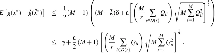
and let ˆˆx∗ be its optimal solution, and g(x)and ˜g(x) be as described in Equations 7 and 8, respectively. The best rank-˜k approximation to Q is ˜Q=UΓUT as given in Section 2.2. A bound on the total error in the QPFS+Nystr¨om approximation is obtained following the reasoning in Fine et al. (2001):
Eg(x∗)−ˆˆg(ˆˆx∗) ≤ Eg(ˆˆx∗)−ˆˆg(ˆˆx∗)
≤ 1
2(1−α)E h
(ˆˆx∗)TQ−Qˆˆ
(ˆˆx∗)i
≤ 1
2E h
kQ−Qˆˆk2kˆˆx∗k22 i
≤ 1
2(M+1)E h
kQ−QˆˆkF
i .
Applying the bound for the Nystr¨om method with uniform sampling without replacement (Equation 10) and the inequalitykQ−Q˜kF ≤trace Q−Q˜
≤(M−˜k)δyields
Eg(x∗)−ˆˆg(ˆˆx∗) ≤ 1
2(M+1)
(M−˜k)δ+ε "
M
r i∈
∑
D(r)Qii !sM
M
∑
i=1Q2ii #1
2
≤ γ+ε
2(M+1) "
M
r i∈
∑
D(r)Qii !sM
M
∑
i=1Q2
ii
#1 2
.
The total error is the sum of the error γobtained from the approximation of the quadratic programming problem in a subspace (Equation 6) and the error due to the Nystr¨om method.
2.3 Summary of the QPFS+Nystr¨om Method
Figure 1 shows a diagram of the proposed feature selection method, which can be summarized as follows:
1. Compute the F vector representing the dependence of each variable with the class.
2. Choose r rows of Q according to some criterion (typically, uniform sampling without replace-ment). Arrange the Q matrix so that these r rows are the first ones. Define the[A B]matrix to be the first r rows of Q.
3. Set the value of theαparameter according to Equation 9.
4. Apply the Nystr¨om method knowing[A B]. Obtain an approximation of the eigenvalues and eigenvectors of Q, ˆQ=U ˆˆΛUˆT.
5. Formulate the quadratic programming (QP) problem in the lower dimensional space ˆˆQ=
ˆˆ UΛˆˆUˆˆT.
6. Solve the QP in the subspace to obtain the solution vector y.
7. Return to the original space via x=U y.ˆˆ
Nyström method
Reduction to lower-dimensional space
QP
Getting back to original space Features
ranking
Figure 1: Diagram of the QPFS algorithm using the Nystr¨om method. [A B]is the upper r×M submatrix of Q.
2.4 Complexity Analysis
As already mentioned, the mRMR method is one of the most successful previous methods for feature selection. The main advantage of the QPFS+Nystr¨om method versus mRMR is the time complexity reduction. The time complexities of mRMR and QPFS both have two components, the time needed to compute the matrices Q and F (Similarity), and the time needed to perform variable ranking (Rank). The computational cost of evaluating correlations or mutual information for all variable pairs is O(NM2)for both mRMR and QPFS. Table 1 shows the time complexities of the three algo-rithms mRMR, QPFS and QPFS+Nystr¨om.
mRMR QPFS QPFS+Nystr¨om
Similarity Rank Similarity Rank Similarity Rank M large
N≪pM O(NM
2) O(M2) O(NM2) O(M3) O(N pM2) O(p2M3)
M medium
N≫pM O(NM
2) O(M2) O(NM2) O(M3) O(NpM2) O(p2M3)
M small
N≫M O(NM
2) O(M2) O(NM2) O(M3) O(NpM2) O(p2M3)
Table 1: Time complexity of algorithms as a function of training set size N, number of variables M, and Nystr¨om sampling rate p. The predominant cost term is indicated in boldface.
2.5 Implementation
We implemented QPFS and mRMR in C using LAPACK for matrix operations (Anderson et al., 1990). Quadratic optimization is performed by the Goldfarb and Idnani algorithm implemented in Fortran and used in the R quadprog package (Goldfarb and Idnani, 1983; Turlach and Weingessel, 2000).
As mentioned in Section 2.1, in general mutual information computation requires estimating density functions for continuous variables. For simplicity, each variable is discretized in three seg-ments(−∞,µ−σ],(µ−σ,µ+σ], and(µ+σ,+∞), where µ is the sample mean of training data and
σits standard deviation. The linear SVM provided by the LIBSVM package (Chang and Lin, 2001) was the underlying classifier in all experiments. A linear kernel is used to reduce the number of SVM parameters, thus making meaningful results easier to obtain. Note that mRMR and QPFS can be used with any classifier learning algorithms. We expect results obtained with linear SVMs to be representative.
3. Experiments
The aim of the experiments described here is twofold: first, to compare classification accuracy achieved using mRMR versus QPFS; and second, to compare their computational cost.
3.1 Experimental Design
The data sets used for experiments are shown in Table 2. These data sets were chosen because they are representative of multiple types of classification problems. with respect to the number of samples, the number of features, and the achievable classification accuracy. Moreover, these data sets have been used in other research on the feature selection task (Hua et al., 2009; Lauer et al., 2007; Lecun et al., 1998; Li et al., 2004; Peng et al., 2005; Zhang et al., 2008; Zhu et al., 2008).
In order to estimate classification accuracy, for the ARR, NCI60, SRBCT and GCM data sets 10-fold cross-validation (10CV) and 100 runs were used (Duda et al., 2000). Mean error rates are comparable to the results reported in Li et al. (2004), Peng et al. (2005), Zhang et al. (2008) and Zhu et al. (2008). In the case of the RAT data set, 120 training samples (61 for test) and 300 runs were used, following Hua et al. (2009). The MNIST data set is divided into training and testing subsets as proposed by Chang and Lin (2001), with 60000 and 10000 patterns respectively. Therefore, cross-validation is not done with MNIST.
Time complexity is measured as a function of training set size (N), dimensionality (M), and the Nystr¨om sampling rate (p= r
M). In all cases, times are averages over 50 runs. In order to measure time complexity as a function of training set size, the number of SRBCT examples was artificially increased 4 times (N=332) and dimensionality reduced to M=140. Time complexity as a function of dimensionality was measured using the original SRBCT data set, that is, with N=83 and M=2308.
Data Set N M C Baseline References Error Rate
ARR 422 278 2 21.81% (Peng et al., 2005; Zhang et al., 2008) (Li et al., 2004; Zhang et al., 2008)
NCI60 60 1123 9 38.67% (Zhu et al., 2008)
SRBCT 83 2308 4 0.22% (Li et al., 2004; Zhu et al., 2008) (Li et al., 2004; Zhang et al., 2008)
GCM 198 16063 14 33.85% (Zhu et al., 2008)
RAT 181 8460 2 8.61% (Hua et al., 2009)
MNIST 60000 780 10 6.02% (Lauer et al., 2007; Lecun et al., 1998)
Table 2: Description of the data sets used in experiments. N is the number of examples, M is the number of variables, and C is the number of classes. Baseline error rate is the rate obtained taking into account all variables. The last column cites papers where the data sets have been mentioned.
0 50 100 150 200 250 15
20 25 30 35 40 45
Number of features
Error Rate (%)
mRMR c=0.01
QPFS MI alpha=0.412 c=0.01 mRMR c=1.0
QPFS MI alpha=0.412 c=1.0 mRMR c=10.0
QPFS MI alpha=0.412 c=10.0
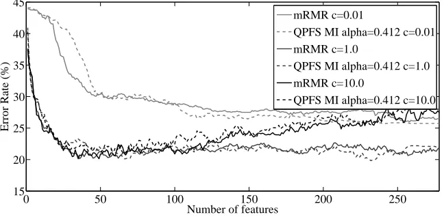
Figure 2: Classification error as a function of the number of features for the ARR data set and different regularization parameter values c in linear SVM. The figure shows that for c=
0.01, the SVM is too regularized. The effect when c=10.0 is the opposite and the SVM overfits the training data. A value of c=1.0 is a good tradeoff.
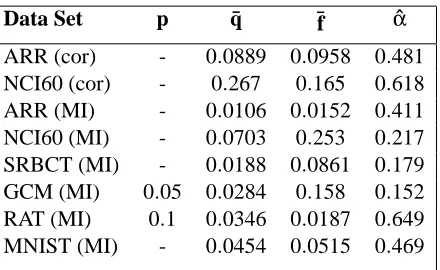
Data Set p ¯q ¯f αˆ
ARR (cor) - 0.0889 0.0958 0.481 NCI60 (cor) - 0.267 0.165 0.618 ARR (MI) - 0.0106 0.0152 0.411 NCI60 (MI) - 0.0703 0.253 0.217 SRBCT (MI) - 0.0188 0.0861 0.179 GCM (MI) 0.05 0.0284 0.158 0.152 RAT (MI) 0.1 0.0346 0.0187 0.649 MNIST (MI) - 0.0454 0.0515 0.469
Table 3: Values of theαparameter for each data set. Correlation (cor) and mutual information (MI) were used as similarity measures for ARR and NCI60 data sets. Only mutual information was used for SRBCT, GCM, RAT and MNIST data sets. p is the subsampling rate in the Nystr¨om method, ¯q is the mean value of the elements of the matrix Q (similarity among each pair of features), and ¯f is the mean value of the elements of the F vector (similarity of each feature with the target class). For the MNIST data set only nonzero values have been considered for the statistics due to the high level of sparsity of its features (80.78% sparsity in average).
3.2 Classification Accuracy Results
The aim of the experiments described in this section is to compare classification accuracy achieved with mRMR and with QPFS, with and without Nystr¨om approximation. The MaxRel algorithm (Peng et al., 2005) is also included in the comparison. Two similarity measures, mutual information (MI) and correlation are considered. Classification error is measured as a function of the number of features. We also give results from a baseline method that does random selection of features, in order to determine the absolute advantage of using any feature selection method.
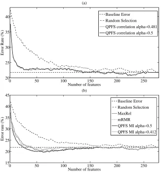
Figure 3 shows the average classification error rate for the ARR data set as a function of the number of features. In Figure 3a, correlation is the similarity measure while mutual information (MI) is applied for Figure 3b. In both cases, the best accuracy is obtained with α=0.5, which means that an equal tradeoff between relevance and redundancy is best. However, accuracies using the values ofαspecified by our heuristic are similar.
Better accuracy is obtained when MI is used, in which case (Figure 3b) the error rate curve for α=0.5 is similar to that obtained with mRMR. The random selection method yields results significantly worse than those obtained with other algorithms. Comparison with this method shows that the other methods provide a significant benefit up to about 150 features.
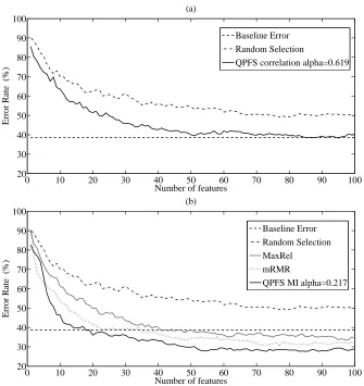
For the NCI60 data set (Figure 4), the best accuracy is obtained when mutual information is used (Figure 4b) andαis set to 0.217 according to Table 3. In this case, the accuracy of QPFS is slightly better than the accuracy of mRMR. The value ofαclose to zero indicates that it is appropriate to give more weight to the quadratic term in QPFS. When correlation is used (Figure 4a), the best accuracy is obtained whenαis set according to Equation 3.
0 50 100 150 200 250 20
25 30 35 40
Number of features
Error Rate (%)
(a)
Baseline Error Random Selection
QPFS correlation alpha=0.481 QPFS correlation alpha=0.5
0 50 100 150 200 250 15
20 25 30 35 40 45
Number of features
Error rate (%)
(b)
Baseline Error Random Selection MaxRel
mRMR
QPFS MI alpha=0.5 QPFS MI alpha=0.412
Figure 3: Classification error as a function of the number of features for the ARR data set. (a) QPFS results using correlation as similarity measure with differentαvalues. (b) MaxRel, mRMR and QPFS results using mutual information as similarity measure and different values ofαfor QPFS.
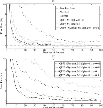
Average error rate for the SRBCT data set and different sampling rates as a function of the num-ber of features is shown in Figure 5. Results for the bestαvalue in the grid{0,0.1,0.3,0.5,0.7,0.9},
α=0.1, and the estimated ˆα=0.179 are shown in Figure 5a. Accuracies for bothαvalues are sim-ilar. The fact that a low value of α is best indicates low redundancy among variables compared to their relevance with the target class. QPFS classification accuracy is similar to that of mRMR. As shown in Figure 5b, when the QPFS+Nystr¨om method is used, the higher the parameter p, the closer the Nystr¨om approximation is to complete diagonalization. QPFS+Nystr¨om gives classifica-tion accuracy similar to that of QPFS when p>0.1.
0 10 20 30 40 50 60 70 80 90 100 20
30 40 50 60 70 80 90 100
Number of features
Error Rate (%)
(a)
Baseline Error Random Selection
QPFS correlation alpha=0.619
0 10 20 30 40 50 60 70 80 90 100 20
30 40 50 60 70 80 90 100
Number of features
Error Rate (%)
(b)
Baseline Error Random Selection MaxRel
mRMR
QPFS MI alpha=0.217
Figure 4: Classification error as a function of number of features for the NCI60 data set. (a) QPFS results using correlation as similarity measure with differentαvalues. (b) MaxRel, mRMR and QPFS results using mutual information as similarity measure and different values ofαfor QPFS.
this data set, which represents a major time complexity reduction given a feature space of 16063 variables.
Another data set with many features is the RAT data set, for which Figure 7 shows results. In this case, QPFS+Nystr¨om gives classification accuracy similar to that of mRMR when the subset size is over 80 and the sampling rate is 10%. Given the good performance of the MaxRel algorithm for this data set, it is not surprising that a largeαvalueα=0.9 or ˆα=0.649 is best, considering also that QPFS withα=1.0 is equivalent to MaxRel.
The MNIST data set has a high number of training examples. Results for it are shown in Figure 8 for the QPFS with α=0.3, the estimation ˆα=0.469 and the QPFS+Nystr¨om with ˆα and p∈
0 10 20 30 40 50 60 70 80 90 100 0
5 10 15 20
Number of features
Error Rate (%)
(a)
Baseline Error MaxRel mRMR
QPFS MI alpha=0.179 QPFS MI alfa=0.1
QPFS+Nystrom MI alpha=0.1 p=0.5
0 10 20 30 40 50 60 70 80 90 100 0
5 10 15 20
Number of features
Error Rate (%)
(b)
QPFS+Nystrom MI alpha=0.1 p=0.01 QPFS+Nystrom MI alpha=0.1 p=0.04 QPFS+Nystrom MI alpha=0.1 p=0.1 QPFS+Nystrom MI alpha=0.1 p=0.5
Figure 5: Error rates using MaxRel, mRMR and QPFS+Nystr¨om methods, with mutual information as similarity measure for the SRBCT data set.
0 50 100 150 200 250 300 350 400 450 30
40 50 60 70 80
Number of features
Error Rate (%)
Baseline Error MaxRel mRMR
QPFS+Nystrom MI alpha=0.1 p=0.03 QPFS+Nystrom MI alpha=0.152 p=0.05
Figure 6: Error rates using MaxRel, mRMR and QPFS+Nystr¨om methods, with mutual information as similarity measure for the GCM data set.
0 50 100 150 200 250 300 350 400 450 5
10 15 20 25 30 35
Number of features
Error Rate (%)
Baseline Error MaxRel mRMR
QPFS+Nystrom MI alpha=0.9 p=0.1 QPFS+Nystrom MI alpha=0.649 p=0.1
Figure 7: Error rates using MaxRel, mRMR and QPFS+Nystr¨om methods, with mutual information as similarity measure for the RAT data set.
Figure 9 shows a grid of 780 pixels arrayed in the same way as the images in the MNIST data sets. A pixel is black if it corresponds to one of the top 100 (Figure 9a) and 350 (Figure 9b) selected features, and white otherwise. Black pixels are more dense towards the middle of the grid, because that is where the most informative features are. Pixels sometimes appear in a black/white/black checkerboard pattern, because neighboring pixels tend to make each other redundant.
10 20 30 40 50 60 70 80 90 100 110 120 5
10 15 20 25 30 35 40
Number of features
Error Rate (%)
Baseline Error MaxRel mRMR MID QPFS MI alpha=0.3
QPFS+Nystrom MI alpha=0.469 p=0.1 QPFS+Nystrom MI alpha=0.469 p=0.2 QPFS+Nystrom MI alpha=0.469 p=0.5 QPFS MI alpha=0.469
Figure 8: Error rates using MaxRel, mRMR and QPFS+Nystr¨om methods, with mutual information as similarity measure for the MNIST data set.
Figure 9: First (a) 100 and (b) 350 features selected by QPFS+Nystr¨om ( ˆα=0.469 and p=0.5) for the MNIST data set (black pixels).
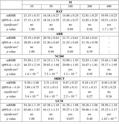
For the NCI60 and SRBCT data sets, the best result is obtained when QPFS is used and it is statistically significantly better than mRMR. When 200 to 400 variables are considered, mRMR and QPFS are not statistically significantly different but the accuracy is not as good as in the case of 100 features, probably due to overfitting. In the case of the GCM data set, the mRMR method is statistically significantly better when fewer than 50 variables are considered. If the number of features is over 100, the accuracy with QPFS is significantly better than with mRMR, and the best performance is obtained in this case. For the ARR data set, mRMR is statistically significantly better than QPFS if fewer than 10 features are considered but the error rate obtained can be improved if more features are taken into account. When more than 50 featues are selected, the two methods are not statistically significantly different. The RAT data set behavior is quite similar. When fewer than 100 features are used, the mRMR algorithm is satatistically better than QPFS, but the error rate can be reduced adding more features. The two algorithms are not statistically significantly different in the other cases, except if more than 400 features are involved in which case QPFS is statistically significantly better than mRMR. Note that the error rates shown for QPFS are obtained with the proposed estimation of ˆα. In some cases, as shown in Figures 3 to 7, thisαvalue is not the best choice.
Beyond simple binary statistical significance, Table 4 indicates that the QPFS method is statis-tically significantly better when the value of ˆαis small. A possible explanation for this finding is the following. When ˆαis small, features are highly correlated with the label ( ¯f ≫q). The mRMR¯ method is greedy, and only takes into account redundancy among features selected in previous iter-ations. When features are highly correlated with the label, then mRMR selects features with high relevance and mostly ignores redundancy. In contrast, QPFS evaluates all variables simultaneously, and always balances relevance and redundancy.
3.2.1 COMPARISON WITHOTHERFEATURESELECTIONMETHODS
The experiments of this work are focused in comparing QPFS with the greedy filter-type method mRMR (difference form, named MID) which also takes into account the difference between redun-dancy and relevance. Nevertheless, other feature selection methods independent of the classifier have been considered in the described experiments:
• mRMR (quotient form, named MIQ) (Ding and Peng, 2005). While in mRMR (MID form) the difference between the estimation of redundancy and relevance is considered, in the case of mRMR (MIQ form) the quotient of both approximations is calculated.
• reliefF (Robnik- ˇSikonja and Kononenko, 2003). The main idea of ReliefF is to evaluate the quality of a feature according to how well it distinguishes between instances that are near to each other. This algorithm is efficient in problems with strong dependencies between attributes.
• Streamwise Feature Selection (SFS) (Zhou et al., 2006). SFS selects a feature if the benefit of adding it to the model is greater than the increase in the model complexity. The algorithm scales well to large feature sets and considers features sequentially for addition to a model making unnecessary to know all the features in advance.
M
10 50 100 200 400
RAT
mRMR 21.15±0.31 16.18±0.27 14.88±0.24 12.81±0.25 10.95±0.23
QPFS ˆα=0.65 27.13±0.33 18.16±0.29 15.24±0.27 12.85±0.26 10.51±0.21
significant? no no no no yes
p value 1.00 1.00 0.89 0.56 1.7×10⁻² ARR
mRMR 25.19±0.65 20.76±0.63 21.71±0.61 21.64±0.61
-QPFS ˆα=0.41 28.05±0.65 21.30±0.65 21.52±0.65 21.76±0.58
-significant? no no no no
-p value 1.00 0.96 0.69 0.39
-NCI60
mRMR 53.50±2.17 34.33±1.74 32.00±1.93 32.83±1.84 33.64±1.80
QPFS ˆα=0.22 46.33±2.19 29.83±1.68 29.00±1.83 34.67±1.81 35.17±1.95
significant? yes yes yes no no
p value 1.6×10⁻³ 7.5×10⁻³ 3.3×10⁻² 0.95 0.96 SRBCT
mRMR 9.38±1.06 2.31±0.51 0.47±0.23 0.24±0.17 0.49±0.30
QPFS ˆα=0.18 3.89±0.75 0.11±0.11 0.05±0.11 0.11±0.11 0.35±0.25
significant? yes yes yes no no
p value 5.4×10⁻⁹ 5.6×10⁻⁵ 2.3×10⁻² 0.27 0.36
GCM
mRMR 54.26±1.19 43.38±1.18 41.38±1.08 38.26±1.06 38.50±1.10
QPFS ˆα=0.15 65.66±1.03 44.11±1.11 39.57±1.24 38.06±1.16 35.23±1.17
significant? no no yes no yes
p value 1.00 0.81 0.037 0.40 1.42×10⁻⁴ Table 4: Average error rates using the mRMR and QPFS methods, for classifiers based on M
fea-tures. The parameter ˆαof the QPFS method is indicated; rows are ordered according to this value. The Nystr¨om approximation was used for the GCM and RAT data sets.
and the average number of features selected by Streamwise Feature Selection. SFS was applied to the binary data sets ARR and RAT and was used only as a feature selection method (a feature generation step was not included).
performance of MIQ in some data sets is not competitive (see, for instance, the ARR and NCI60 results). The accuracy of QPFS+Nystr¨om (p=0.2) is good if a high enough number of features is used, and it has lower computational cost than mRMR and QPFS.
Regarding SFS, Table 6 shows that SFS provides a competitive error rate for the ARR data set with few features (around 11) but its effectiveness in the RAT data set is improved by other feature selection algorithms when more than 6 attributes are considered. It is noticeable the efficiency of SFS getting acceptable accuracies using a small number of features.
ReliefF and SFS are feature selection methods which need to establish the value of some param-eters like in QPFS. In ReliefF all instances were used (not random subsampling) and the number of neighbors was set to 3 for all data sets, except for MNIST where 10 neighbors were considered. In the case of the SFS algorithm, the default values (wealth=0.5 and△α=0.5) were used.
3.3 Time Complexity Results
Since the previous subsection has established the effectiveness of the QPFS method, it is useful now to compare mRMR and QPFS experimentally with respect to time complexity. As stated in Table 1 in Section 2.4, the running times of mRMR and QPFS with and without Nystr¨om all depend linearly on N when M and p are fixed. In order to confirm experimentally this theoretical dependence, time consumption as a function of the number of training examples is measured on the SRBCT data set.
Figure 10a shows the time consumed for the modified SRBCT data set, averaged over 50 runs, as a function of the number of samples, N, for the mRMR, QPFS and QPFS+Nystr¨om methods.
As expected, both mRMR and QPFS show a linear dependence on the number of patterns. For QPFS+Nystr¨om, Table 1 shows that the slope of this linear dependence is proportional to the sampling rate p. Over the range p=0.01 to p=0.5, a decrease in p leads to a decrease in the slope of the linear dependence on N. Therefore, although all algorithms are linearly dependent on N, the QPFS+Nystr¨om is computationally the most efficient. The time cost advantage increases with increasing number of training examples because the slope is greater for mRMR than for QPFS.
The next question is the impact on performance of the number of features, M. Table 1 shows that mRMR and QPFS have quadratic and cubic dependence on M, respectively. However, the QPFS+Nystr¨om cubic coefficient is proportional to the square of the sampling rate. When small value of p are sufficient, which is the typical case, the cubic terms are not dominant.
These results are illustrated in the experiments shown in Figure 10b. This figure shows the average time cost for the SRBCT data set as a function of the problem dimension, M, for the mRMR, QPFS, and QPFS+Nystr¨om methods. As expected from Table 1, mRMR and QPFS empirically show quadratic and cubic dependence on problem dimension. QPFS+Nystr¨om shows only quadratic dependence on problem dimension, with a decreasing coefficient for decreasing p values. In all cases, a t-test has been used to verify the order of the polynomial that best fits each curve by least-squares fitting (Neter and Wasserman, 1974). Overall, for small Nystr¨om sampling rates, QPFS+Nystr¨om is computationally the most efficient.
Data Set Method M
10 20 40 50 100 200 400
MaxRel 27.48 24.68 21.70 20.82 20.31 21.73 -MID 25.19 22.99 20.64 20.76 21.71 21.64 -ARR MIQ 29.79 27.78 23.89 23.32 21.53 21.74 -reliefF 30.64 24.48 21.54 21.34 20.90 21.66 -QPFS 28.05 23.72 22.39 21.30 21.52 21.76 -MaxRel 61.33 49.83 40.00 38.67 34.83 35.50 34.17 MID 53.50 41.50 36.33 34.33 32.00 32.83 33.67 NCI60 MIQ 56.50 47.50 38.83 38.17 32.83 35.50 35.17 reliefF 56.93 54.17 48.49 48.49 38.07 32.13 34.36 QPFS 46.33 36.00 33.00 29.83 29.00 34.67 35.17 MaxRel 21.58 14.33 6.36 4.51 2.19 0.24 0.13 MID 9.39 3.33 2.01 2.31 0.47 0.24 0.49 SRBCT MIQ 10.11 2.18 0.47 0.72 0.24 0.25 0.72 reliefF 6.38 4.18 1.65 1.79 0.96 0.40 0.40 QPFS 3.89 1.57 0.97 0.11 0.05 0.11 0.35 MaxRel 79.32 60.78 48.46 45.58 40.98 39.98 38.77 MID 54.26 48.45 44.16 43.38 41.38 38.26 35.50 GCM MIQ 79.32 56.48 46.64 43.96 41.80 38.46 38.05 reliefF 61.25 51.61 46.36 43.83 39.35 39.75 37.08 QPFS+N p=0.05 65.66 54.72 46.09 44.11 39.57 38.06 35.26 MaxRel 19.95 17.32 15.40 15.16 14.34 13.54 11.97 MID 21.15 18.46 16.53 16.18 14.88 12.81 10.95 RAT MIQ 23.69 19.62 17.23 16.61 15.07 12.46 10.96 reliefF 22.16 20.40 17.44 16.45 13.68 11.43 9.85 QPFS+N p=0.1 27.13 21.89 19.02 18.16 15.24 12.85 10.51 MaxRel 59.19 40.98 25.77 22.5 12.09 7.64 6.72 MID 53.39 29.37 19.56 17.40 11.72 7.55 6.66 MNIST MIQ 51.69 25.98 11.79 10.87 7.78 6.90 6.33 reliefF 50.91 40.20 23.81 19.56 12.31 8.47 6.86 QPFS+N p=0.2 57.00 35.39 23.62 20.48 11.31 7.71 6.54
Table 5: Error rates for different feature selection methods and Linear SVM. The best result in each case is marked in bold. QPFS+N indicates that the Nystr¨om approximation is used in the QPFS method and p represents the subsampling rate in Nystr¨om method. In all cases, the
αparameter of QPFS is set to ˆα.
4. Conclusions
Data Set Number of Selected Features (average) Error rate (%)
ARR 10.75±0.155 23.34±0.63
RAT 6.12±0.13 22.87±0.33
Table 6: Streamwise Feature Selection error rates.
0 50 100 150 200 250 300 0 0.05 0.1 0.15 0.2 0.25 0.3 0.35
Number of Patterns (N)
Average time cost (seconds)
0 500 1000 1500 0 0.5 1 1.5 2 2.5 3 3.5 4 Dimension (M)
Average time cost (seconds)
0 0.2 0.4 0.6 0.8 0 1 2 3 4 5 6 7 8 9 10
Subsampling rate (p)
Average time cost (seconds)
mRMR QPFS alpha=0.1
QPFS+Nystrom alpha=0.1 p=0.01 QPFS+Nystrom alpha=0.1 p=0.05 QPFS+Nystrom alpha=0.1 p=0.1 mRMR
QPFS alpha=0.1 QPFS+N alpha=0.1 p=0.01 QPFS+N alpha=0.1 p=0.25 QPFS+N alpha=0.1 p=0.5
M=100 M=300 M=400 M=500
Figure 10: Time cost in seconds for mRMR and QPFS as a function of: (a) the number of patterns, N; (b) the dimension, M; and (c) the sampling rate, p. QPFS+N indicates that the Nystr¨om approximation is used in the QPFS method.
on the optimization of a quadratic function that is reformulated in a lower-dimensional space using the Nystr¨om approximation (QPFS+Nystr¨om). The QPFS+Nystr¨om method, using either Pearson correlation coefficient or mutual information as the underlying similarity measure, is computation-ally more efficient than the leading previous methods, mRMR and MaxRel.
With respect to classification accuracy, the QPFS method is similar to MaxRel and mRMR when mutual information is used, and yields slightly better results if there is high redundancy. In all experiments, mutual information yields better classification accuracy than correlation, presumably because mutual information better captures nonlinear dependencies. Small sampling rates in the Nystr¨om method still lead to reasonable approximations of exact matrix diagonalization, sharply reducing the time complexity of QPFS. In summary, the new QPFS+Nystr¨om method for selecting a subset of features is a competitive and efficient filter-type feature selection algorithm for high-dimensional classifier learning problems.
Acknowledgments
References
E. Anderson, Z. Bai, J. Dongarra, A. Greenbaum, A. McKenney, J. Du Croz, S. Hammarling, J. Demmel, C. H. Bischof, and Danny C. Sorensen. LAPACK: a portable linear algebra library for high-performance computers. In SC, pages 2–11, 1990.
R. Bekkerman, N. Tishby, Y. Winter, I. Guyon, and A. Elisseeff. Distributional word clusters vs. words for text categorization. Journal of Machine Learning Research, 3:1183–1208, 2003.
D.P. Bertsekas. Nonlinear Programming. Athena Scientific, September 1999.
L. Breiman, J.H. Friedman, R.A. Olshen, and C.J.Stone. Classification and Regression Trees. Chap-man & Hall/CRC, January 1984.
C. Chang and C. Lin. LIBSVM: a library for support vector machines, 2001. Software available at
http://www.csie.ntu.edu.tw/˜cjlin/libsvm.
T. M. Cover and J. A. Thomas. Elements of information theory. Wiley-Interscience, New York, NY, USA, 1991.
T.M. Cover. The best two independent measurements are not the two best. IEEE Trans. Systems, Man, and Cybernetics, 4:116–117, 1974.
C. Ding and H. Peng. Minimum redundancy feature selection from microarray gene expression data. J Bioinform Comput Biol, 3(2):185–205, April 2005.
R. O. Duda, P.E. Hart, and D. G. Stork. Pattern Classification (2nd Edition). Wiley-Interscience, November 2000.
S. Fine, K. Scheinberg, N. Cristianini, J. Shawe-Taylor, and B. Williamson. Efficient SVM training using low-rank kernel representations. Journal of Machine Learning Research, 2:243–264, 2001.
G. Forman. BNS feature scaling: an improved representation over TF-IDF for SVM text classifi-cation. In CIKM ’08: Proceeding of the 17th ACM conference on Information and knowledge mining, pages 263–270, New York, NY, USA, 2008. ACM.
G. Forman. An extensive empirical study of feature selection metrics for text classification. J. Mach. Learn. Res., 3:1289–1305, 2003.
C. Fowlkes, S. Belongie, and J. Malik. Efficient spatiotemporal grouping using the Nystr¨om method. In Proc. IEEE Conf. Comput. Vision and Pattern Recognition, pages 231–238, 2001.
D. Goldfarb and A. Idnani. A numerically stable dual method for solving strictly convex quadratic programs. Mathematical Programming, 27(1):1–33, 1983.
I. Guyon. An introduction to variable and feature selection. Journal of Machine Learning Research, 3:1157–1182, 2003.
J. Hua, W. D. Tembe, and E. R. Dougherty. Performance of feature-selection methods in the classi-fication of high-dimension data. Pattern Recogn., 42(3):409–424, 2009.
A. K. Jain, R. P. W. Duin, and J. Mao. Statistical pattern recognition: A review. IEEE Trans. Pattern Anal. Mach. Intell., 22(1):4–37, January 2000.
G. John, R. Kohavi, and K. Pfleger. Irrelevant features and the subset selection problem. In Machine Learning: Proceedings of the Eleventh International Conference, San Francisco, 1994.
R. Kohavi and G. H. John. Wrappers for feature subset selection. Artificial Intelligence, 97(1-2): 273–324, 1997.
S. Kumar, M. Mohri, and A. Talwalkar. Sampling techniques for the Nystr¨om method. In Pro-ceeding of the 12th International Conference on Artificial Intelligence and Statistics (AISTATS), 2009.
P. Langley. Selection of relevant features in machine learning. In Proceedings of the AAAI Fall symposium on relevance, pages 140–144. AAAI Press, 1994.
F. Lauer, C. Y. Suen, and G. Bloch. A trainable feature extractor for handwritten digit recognition. Pattern Recogn., 40(6):1816–1824, 2007.
Y. Lecun, Y. Bengio, and P. Haffner. Gradient-based learning applied to document recognition. In Proceedings of the IEEE, pages 2278–2324, 1998.
R. Leitner, H. Mairer, and A. Kercek. Real-time classification of polymers with NIR spectral imag-ing and blob analysis. Real-Time Imagimag-ing, 9:245 – 251, 2003.
T. Li, C. Zhang, and M. Ogihara. A comparative study of feature selection and multiclass classifica-tion methods for tissue classificaclassifica-tion based on gene expression. Bioinformatics, 20:2429–2437, 2004.
K. Momen, S. Krishnan, and T. Chau. Real-time classification of forearm electromyographic signals corresponding to user-selected intentional movements for multifunction prosthesis control. Neu-ral Systems and Rehabilitation Engineering, IEEE Transactions on, 15(4):535–542, Dec. 2007.
J. Neter and W. Wasserman. Applied Linear Statistical Models. Richard D. Irwin, INC., 1974.
H. Peng, F. Long, and C. Ding. Feature selection based on mutual information: criteria of max-dependency, max-relevance, and min-redundancy. IEEE Trans. Pattern Anal. Mach. Intell, 27: 1226–1238, 2005. Software available athttp://research.janelia.org/peng/proj/mRMR/.
M. Robnik- ˇSikonja and I. Kononenko. Theoretical and empirical analysis of ReliefF and RReliefF. Mach. Learn., 53(1-2):23–69, 2003.
J. Rodriguez, A. Goni, and A. Illarramendi. Real-time classification of ECGs on a PDA. IEEE Transactions on Information Technology in Biomedicine, 9(1):23–34, 2005.
B. A. Turlach and A. Weingessel. The quadprog package, version 1.4-11, 2000. Available electron-ically atcran.r-project.org/web/packages/quadprog/index.html.
J. Weston, S. Mukherjee, O. Chapelle, M. Pontil, T. Poggio, and V. Vapnik. Feature selection for SVMs. In Advances in Neural Information Processing Systems 13, pages 668–674. MIT Press, 2001.
C. K. I. Williams and M. Seeger. Using the Nystr¨om method to speed up kernel machines. In Advances in Neural Information Processing Systems 13, pages 682–688. MIT Press, 2001.
L. Yu and H. Liu. Feature selection for high-dimensional data: A fast correlation-based filter solu-tion. In Proceedings of the Twentieth International Conference on Machine Learning (ICML-03), 2003.
Y. Zhang, C. Ding, and T. Li. Gene selection algorithm by combining reliefF and mRMR. BMC Genomics, 9(Suppl 2), 2008.
J. Zhou, D. P. Foster, R. A. Stine, and L. H. Ungar. Streamwise feature selection. J. Mach. Learn. Res., 7:1861–1885, 2006.
![Figure 1: Diagram of the QPFS algorithm using the Nystr¨om method. [A B] is the upper r × Msubmatrix of Q.](https://thumb-us.123doks.com/thumbv2/123dok_us/9825385.1968530/10.612.117.497.429.569/figure-diagram-qpfs-algorithm-using-nystr-method-msubmatrix.webp)