Estimation of Sparse Binary Pairwise Markov Networks using
Pseudo-likelihoods
Holger H¨ofling [email protected]
Department of Statistics Stanford University Stanford, CA 94305, USA
Robert Tibshirani [email protected]
Depts. of Health, Research & Policy and Statistics Stanford University
Stanford, CA 94305, USA
Editor: Michael Jordan
Abstract
We consider the problems of estimating the parameters as well as the structure of binary-valued Markov networks. For maximizing the penalized log-likelihood, we implement an approximate procedure based on the pseudo-likelihood of Besag (1975) and generalize it to a fast exact algo-rithm. The exact algorithm starts with the likelihood solution and then adjusts the pseudo-likelihood criterion so that each additional iterations moves it closer to the exact solution. Our results show that this procedure is faster than the competing exact method proposed by Lee, Gana-pathi, and Koller (2006a). However, we also find that the approximate pseudo-likelihood as well as the approaches of Wainwright et al. (2006), when implemented using the coordinate descent procedure of Friedman, Hastie, and Tibshirani (2008b), are much faster than the exact methods, and only slightly less accurate.
Keywords: Markov networks, logistic regression, L1penalty, model selection, Binary variables
1. Introduction
In recent years a number of authors have proposed the estimation of sparse undirected graphical models for continuous as well as discrete data through the use of L1 (lasso) regularization. For continuous data, one assumes that the observations have a multivariate Gaussian distribution with mean µ and covariance matrixΣ. Then an L1 penalty is applied toΘ=Σ−1. That is, the penalized log-likelihoodℓ(Θ)−ρ||Θ||1is maximized, whereℓis the Gaussian log-likelihood,||Θ||1is the sum of the absolute values of the elements ofΘ andρ≥0 is a user-defined tuning parameter. Several papers proposing estimation procedures for this Gaussian model have been published. Meinshausen and B¨uhlmann (2006) develop a lasso based method for estimating the graph structure and give theoretical consistency results. Yuan and Lin (2007), Banerjee et al. (2008) and Dahl et al. (2008) as well as Friedman, Hastie, and Tibshirani (2008a) propose algorithms for solving this penalized log-likelihood with the procedure in Friedman, Hastie, and Tibshirani (2008a), the graphical lasso, being especially fast and efficient.
X1 X2 X3
X4
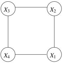
Figure 1: A simple graph for illustration.
x1 x2 x3 x4
1 1 1 0
1 1 0 1
0 0 1 0
1 1 0 1
1 1 1 0
1 1 0 1
0 0 1 0
1 1 0 1
0 1 1 0
1 1 0 1
Table 1: Sample data for graph of Figure 1
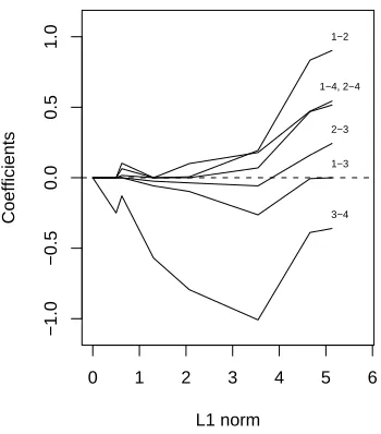
special class as well as more general Markov networks was proposed by Lee, Ganapathi, and Koller (2006a). This problem is more difficult than the continuous Gaussian version because of the need to compute the first and second moments under the model, which are derivatives of the log-partition function. Figure 1 shows an example, and Table 1 shows some sample data from this graph. Given this data and a model for binary graphical data (detailed later), we would like to a) infer a structure something like that of Figure 1, and b) estimate the link parameters itself. For the data in Table 1, Figure 2 shows the path of solutions for varying penalty parameter. Most edges for L1-norm≤2 are correctly identified as in the graph in Figure 1. However, edge(1,3)is absent in the true model but included in the L1penalized model relatively early.
Our main focus in this paper is to develop and implement fast approximate and exact proce-dures for solving this class of L1-penalized binary pairwise Markov networks and compare the accuracy and speed of these to other methods proposed by Lee, Ganapathi, and Koller (2006a) and Wainwright et al. (2006). Here, by “exact” procedures we refer to algorithms that find the exact maximizer of the penalized log-likelihood of the model whereas “approximate” procedures only find an approximate solution.
0 1 2 3 4 5 6
−1.0
−0.5
0.0
0.5
1.0
L1 norm
Coefficients
1−2
1−3 1−4, 2−4
2−3
3−4
Figure 2: Toy example: profiles of estimated edge parameters as the penalty parameter is varied.
the added advantage that it can be used as a building block to a new algorithm for maximizing the penalized log-likelihood exactly. The adjustments necessary to achieve this are described in Section 4. Finally, Section 5 discusses the results of the simulations with respect to speed and accuracy of the competing algorithms.
2. The Model and Competing Methods
In this section we briefly outline the competing methods for maximizing the penalized log-likelihood. Apart from the method proposed in Lee, Ganapathi, and Koller (2006a), which we already men-tioned above, we also discuss a very simple solution that was presented in Wainwright et al. (2006). We first describe the underlying model in more detail. Consider data generated under the Ising model
p(x,Θ) =exp "
∑
s∈V
θsxs+
∑
(s,t)∈Eθstxsxt−Ψ(Θ)
# .
for a single observation x= (x1, . . . ,xp)T ∈ {0,1}p and model parametersθsandθst for s,t∈V =
{1, . . . ,p}. Here, V denotes the vertices and E the edges of a graph. Ψ(Θ) is the normalization constant, which is also known as the log-partition function. By settingθst=0 for (s,t)6∈E, and using the fact that x is a binary vector we can write the log-likelihood as
l(x,Θ) =log p(x,Θ) =
p
∑
s≥t≥1
whereΘis a symmetric p×p matrix withθss=θsfor s=1, . . . ,p. Note that for notational conve-nience, we do not distinguish betweenθstandθtsand therefore we enforce symmetry ofΘalthough the log-likelihood only uses the lower-triangular matrix ofΘ. For the L1-penalty let R be a p×p lower triangular matrix of penalty parameters. The penalized log-likelihood for all N observations is
p
∑
s≥t≥1
(XTX)stθst−NΨ(Θ)−N||R∗Θ||1
where∗denotes component-wise multiplication.
The algorithms that we will discuss in the following sections could be generalized to more general categorical variables or higher order interaction terms than those included in the Ising model. However, as we will see, solving these problems exactly is already computationally demanding in the pairwise binary case so that we chose not to adapt the algorithms to these more general settings.
2.1 The Lee, Ganapathi, and Koller (2006a) Method
The penalized log-likelihood is a concave function, so standard convex programming techniques can be used to maximize it. The main difficulty is that the log-partition functionΨ(Θ)is the sum over 2p elements, and therefore it is computationally expensive to calculate Ψ or its derivatives in general. However, for sparse matrices Θ, algorithms such as the junction tree algorithm exist that can calculateΨand its derivatives efficiently. Therefore, it is especially important to maintain sparsity of Θ for any optimization method. Lee, Ganapathi, and Koller (2006a) achieve this by optimizing the penalized log-likelihood only over a set F of active variables which they gradually enlarge until an optimality criterion is satisfied.
To be more precise, they start out with a set of active variables F =F0 (e.g., the diagonal of
Θif it is unpenalized). Using either conjugate gradients or BFGS, the penalized log-likelihood is maximized over the set of variables F. Then one of the currently inactive variables is selected by the grafting procedure (see Perkins et al., 2003) and added to the set F. These steps are repeated until grafting does not add any more features. The algorithm can be used for more general Markov networks, but for ease of implementation they choose to work with binary random variables and we do the same as well.
Their procedure provides an exact solution to the problem when the junction tree algorithm is used to calculate Ψ(Θ) and its derivatives. In their implementation, however, they used loopy belief propagation, which is faster on denser matrices, but only provides approximate results. In their method as well as ours, any procedure to evaluate Ψ(Θ) can be “plugged in” without any further changes to the rest of the algorithm; we decided to evaluate the speed and performance of only the exact algorithms. The relative performance of an approximate method using loopy belief propagation would likely be similar. They also provide a proof that under certain assumptions and using the L1regularized log-likelihood, it is possible to recover the true expected log-likelihood up to an errorε.
2.2 The Wainwright et al. (2006) Method
Then set ˜θss=β0, the intercept of the logistic regression, and ˜θst=βt, whereβt is the coefficient associated with xt in the regression.
In the outline above, we assumed thatΘis a symmetric matrix. However, due to the way it was constructed, ˜Θis not necessarily symmetric. We investigate two methods for symmetrizing ˜Θ. The first way is to defineΘas
θst=θts= (
˜
θst if|θst˜ |>|θts˜ | ˜
θts if|θst˜ | ≤ |θts˜ |
which we call “Wainwright-max”. Similarly, “Wainwright-min” is defined by
θst=θts= (
˜
θst if|θst˜ |<|θts˜ | ˜
θts if|θst˜ | ≥ |θts˜ |.
Wainwright et al. (2006) mainly intended their method to be used in order to estimate the presence or absence of an edge in the underlying graph of the model. They show that under certain assumptions, their method correctly identifies the non-zero edges in a Markov graph, as N→∞even for increasing number of parameters p or neighborhood sizes of the graph d, as long as N grows more quickly than d3log p (see Wainwright et al., 2008). Due to the simplicity of the method it is obvious that it could also be used for parameter estimation itself and here we will compare its performance in these cases to the pseudo-likelihood approach proposed below and the exact solution of the penalized log-likelihood. Furthermore, as an important part of this article is the comparison of the speeds of the underlying algorithms, we implement their method, using the fast coordinate descent algorithm for logistic regression with a lasso penalty (see Friedman, Hastie, and Tibshirani, 2008b).
3. Pseudo-likelihood Model
In this section we first introduce an approximate method to infer the structure of the graph that is based on pseudo-likelihoods (Besag, 1975). As we will see in the simulations section, the results are very close to the exact solution of the penalized log-likelihood. In the next section, we use the pseudo-likelihood model to design a very fast algorithm for finding an exact solution for the penalized Ising model.
The main computational problem in the Ising model is the complexity of the partition function. One possibility in this case is to solve an approximate version of the likelihood instead. Approaches of this kind have been proposed in various papers in the statistical literature before, for example the pseudo-likelihood approach of Besag (Besag, 1975) and the treatments of composite likelihoods in Lindsay (1998) and Cox and Reid (2004) among others. Here, we want to apply the approximation proposed in Besag (1975) to our problem. This approach is also related to the method of Wainwright et al. (2006), however instead of performing separate logistic regressions for every column of the parameter matrixΘ, the pseudo-likelihood approach here allows us to estimate all parameters at the same time. This way, the resulting matrixΘis symmetric and no additional step like the max or min-rule described above is necessary. The log-pseudo-likelihood is then given by
˜l(Θ|x) =
p
∑
s=1
log p(xs,Θ|x\s)
with
log p(xs,Θ|x\s) =xi(θss+
∑
t6=sHere,Ψs(x,Θ)is the log-normalization constant when conditioning xson the other variables, which
is exactly the same as in logistic regression with a logit link-function, that is,
Ψs(x,Θ) =log(1+exp(θss+
∑
t6=s
xtθst))
where as above for notational convenience we setθst=θts for t6=s. Putting all this together, the pseudo-likelihood for a single observation x is given by
˜l(Θ|x) =
p
∑
s=1
p
∑
t=1
xsxtθst− p
∑
s=1
Ψs(x,Θ).
In the usual way, the likelihood for all N observations is given by the sum of the pseudo-likelihood of the individual observations
˜l(Θ|X) =
N
∑
k=1 ˜l(Θ|xk)
where xk is the kth row of matrix with observations X∈RN×p.
As this is just a sum of logistic likelihoods, the pseudo-likelihood is a concave function and therefore the L1-penalized pseudo-likelihood
N
∑
k=1
˜l(Θ|xk)−N||S∗Θ||1
is concave as well. Here S=2R−diag(R)and is chosen to be roughly equivalent to the penalty terms in the penalized log-likelihood. The penalty term is doubled on the off-diagonal, as the derivative of the pseudo-likelihood on the off-diagonal is roughly twice as large as the derivative of the log-likelihood (see Equation 1).
3.1 Basic Optimization Algorithm
Due to its simple structure, a wide range of standard convex programming techniques can be used to solve this problem, although the non-differentiability of the L1penalty poses a problem. Here, we want to use a local quadratic approximation to the pseudo-likelihood. As the number of variables is p(p+1)/2, the Hessian could get very large, we restrict our quadratic approximation to have a diagonal Hessian.
In order to construct the approximation, we need the first and second derivative of ˜l w.r.t θst. These are
∂˜l
∂θst =2(XTX)st−(ˆpTsX)t−(ˆptTX)s s6=t, (1) ∂˜l
∂θss = (XTX)ss− N
∑
k=1 ˆ psk
where 1−pˆsk=1/(1+exp(θss+∑s6=tXktθst)). The second derivatives are ∂2˜l
(∂θst)2 =−(X
Tdiag(ˆp
s)diag(1−ˆps)X)tt−(XTdiag(ˆpt)diag(1−ˆpt)X)ss s6=t, ∂2˜l
(∂θss)2 =−
N
∑
k=1 ˆ
Algorithm 1: Estimation for L1penalized pseudo-likelihood
ifΘ(0)not given then
SetΘ(0)=diag(logit(ˆp(0)))where ˆp(s0)=N1∑Nk=1xks end
Set k:=0;
while not converged do
With current estimateΘ(k), define local approximation fΘ(k)(Θ)to ˜l−N||S∗Θ||1; Find solutionΘ∗of fΘ(k)(Θ);
Perform backtracking line search on the line fromΘ(k)toΘ∗to findΘ(k+1); Set k:=k+1
end
Assume that at the k-th step the parameter estimate isΘ(k). Then define the local approximation to ˜l(Θ|X)−N||S∗Θ||1as
fΘ(k)(Θ) =C+
∑
s≥t∂˜l
∂θst(θst−θ(stk)) +
1 2
∂2˜l
(∂θst)2(θst−θ
(k)
st )2−N||S∗Θ||1
where C is some constant. As stated above, this is just a quadratic approximation with linear term equal to the gradient of ˜l and a diagonal Hessian with diagonal elements equal to the diagonal of the Hessian of ˜l. The main reasons for using this simple structure are that it keeps the computation complexity per iteration low and it is very easy to solve this L1 penalized local approximation. Let
˜
Θbe the minimizer of the unpenalized fΘ(k)(Θ), then
˜
θst=θ(stk)− ∂˜l ∂θst
∂2˜l
(∂θst)2
.
As the Hessian is diagonal, the L1-penalized solutionΘ∗of fΘ(k)(Θ)can be obtained by soft
thresh-olding as
θ∗
st=sign(θst˜ )
˜
θst−sst/ ∂2˜l (∂θst)2
+
.
UsingΘ∗, the next stepΘ(k+1) can now be obtained by, for example, a backtracking line search. The whole algorithm can be seen in Algorithm 1 and a proof of convergence that closely follows Lee, Lee, Abbeel, and Ng (2006b) is given in the appendix.
3.2 Speed Improvements
In practice, there are several things that can be done to speed up the algorithm given above. First of all, as Θ will in general be sparse, all computations to calculate ˆp should exploit this sparse structure. However, the sparseness ofΘcan also be used in another way:
3.2.1 USINGACTIVEVARIABLES
Algorithm 2: Pseudo-likelihood algorithm using active variables
ifΘ(0)not given then
SetΘ(0)=diag(logit(ˆp(0)))where ˆp(s0)=N1∑Nk=1xks end
Set k:=0;
Set
A
={(s,t): s≥t,θst6=0}as active variables;repeat
while not converged over variables in
A
doFindΘ(k+1)using local approximation over variables in
A
;Set k:=k+1;
end
Set
A
=n
(s,t):θst6=0 or
∂˜l ∂θst
>sst
o ;
until
A
did not change ;efficient, it is possible to move variables that are zero only once in a while. Several different kinds of methods have been proposed to exploit this situation, for example grafting (Perkins et al., 2003) and the implementation of the penalized logistic regression in Friedman, Hastie, and Tibshirani (2008b) among others. In our case here, we use an outer and an inner loop. The outer loop decides which variables are active. The inner loop then optimizes over only the active variables until convergence occurs. Active variables are those that are either non-zero, or that have a gradient large enough so that they would become non-zero in the next step. More details are given in Algorithm 2.
When using this method, convergence is still guaranteed. In the outer loop, the criterion chooses variables to be active that are either non-zero already or will be non-zero after one step of the local approximation over all variables. Therefore, if the active set stays the same, no variables would be moved in the next step as all active variables are already optimal and therefore, we have a solution over all variables. However, if the active set changes, the inner loop is guaranteed to improve the penalized pseudo-likelihood and find the optimum for the given set of active variables. As there are only a finite number of different active variables sets, the algorithm has to converge after a finite number of iterations of the outer loop.
3.2.2 SUBSTITUTING THELINESEARCH
4. Exact Solution Using Pseudo-likelihood
We now turn to our new method for optimizing the penalized log-likelihood. As the log-likelihood is a concave function, there are several standard methods that can be used for maximizing it, for example, gradient descent, BFGS and Newton’s method among others. For each step of these methods, the gradient of the log-likelihood has to be calculated. This requires the evaluation of the partition function and its derivatives, which is computationally much more expensive than any other part of the algorithms. Taking this into considerations, the standard methods mentioned above have the following drawbacks:
Gradient descent: It can take many steps to converge and therefore require many evaluations of
the partition function and its derivatives (using the junction tree algorithm). Also, it does not control the number of non-zero variables in intermediate steps well to which the runtime of the junction tree algorithm is very sensitive. Therefore, intermediate steps can take very long.
BFGS: Takes less steps than gradient descent, but similar to gradient descent, intermediate steps
can have more non-zero variables than the solution. Thus, same as above, computations of intermediate steps can be slow.
Newton’s method: In order to locally fit the quadratic function, the second derivatives of the
log-likelihood are needed. Computing these is computationally prohibitive.
Lee, Ganapathi, and Koller (2006a) use the BFGS method only on a set of active variables onto which additional variables are “grafted” until convergence. This mitigates the problem of slow intermediate steps and makes using BFGS feasible. However, this comes at the expense of an increased total number of steps, as only one variable at a time is being grafted. Here, we want to use the pseudo-likelihood in a new algorithm for maximizing the penalized log-likelihood.
The functional form of the pseudo-likelihood is by its definition closely related to the real like-lihood and in Section 5 we will see that its solutions are also very similar, indicating that it approxi-mates the real likelihood reasonably well. Furthermore, we can also maximize the pseudo-likelihood very quickly. We want to leverage this by using a quasi-Newton method in which we fit a “tilted” pseudo-likelihood instead of a quadratic function. Specifically, among all functions of the form
fΘ(k)=
1
2˜l+s
∑
≥tast(θst−θ (k) st )−γ∑
s≥t
(θst−θ(stk))2−N||R∗Θ||1,
we fit the one that atΘ(k)is a first order approximation to the penalized log-likelihood l. Essen-tially, fΘ(k) is an L1-penalized pseudo-likelihood with an added linear term as well as a very simple quadratic term for someγ>0. Here, astwill be chosen so that the sub-gradient is equal to the
In particular, for the approximation atΘ(k), choose astsuch that
fΘ(k)=
1
2 ˜l(Θ|X) +s
∑
>t(θst−θ (k) st )
(ˆp(Θ(k))sTX)t+ (ˆp(Θ(k))tTX)s−2·N·wst(Θ(k))
+
+
∑
s
(θss−θ(ssk))
∑
kˆ
psk(Θ(k)) + (XTX)ss−2·N·wss(Θ(k))
!! −
−
∑
s≥t
γ(θst−θ(stk))2−N||R∗Θ||1
where W is a matrix with elements wst(Θ) = ∂θ∂Ψst(Θ) =EΘ(xsxt)is the derivative of the partition
function and ˆpsis as defined in the pseudo-likelihood section.
For the algorithm, we need an initial parameter estimateΘ(0), which we pick as follows: Let Z(θ) = eθ
1+eθ be the logistic function and let Z
−1denote its inverse. Then choose
θ(0) st =
(
0 if s6=t
Z−1 1
N∑ N k=1xks
if s=t. In this case we than have ˆpsk=N1∑Nk=1xks ∀k and also
Wst=
( 1
N∑ N k=1xks
1
N∑ N k=1xkt
if s6=t 1
N∑ N k=1xks
if s=t and together withγ=0 we then get that
fΘ(0)=
1
2˜l(Θ|X)−N||R∗Θ||1
and thus just a regular pseudo-likelihood step. The only slight difference is that in this case the penalty term on the diagonal is twice as large as in the pseudo-likelihood case presented above. However, in practice we recommend not to penalize the diagonal at all, so that this difference vanishes. Therefore, this algorithm is a natural extension of the pseudo-likelihood approach that starts out by performing a regular pseudo-likelihood calculation and then proceeds to converge to the solution by a series of adjusted pseudo-likelihood steps.
The algorithm for maximizing the penalized log-likelihood is now very similar to the one pre-sented for maximizing the penalized pseudo-likelihood. Assume our current estimate isΘ(k). Then approximate the log-likelihood locally by fΘ(k) and find the maximizerΘ∗ of fΘ(k). This is
essen-tially the pseudo-likelihood and the algorithm presented above can easily be adjusted to accommo-date the additional terms. Now, using a line search on the line betweenΘ(k)andΘ∗, find the next estimateΘ(k+1). This algorithm is guaranteed to converge by the same argument as the pseudo-likelihood algorithm. The proof that fΘ(k) approximates l at Θ(k) to first order can be found in
Appendix B, which is a prerequisite for the convergence proof of the algorithm in Appendix A.
4.1 Speed Improvement
Algorithm 3: Likelihood algorithm using active variables
ifΘ(0)not given then
SetΘ(0)=diag(logit−1(ˆp(0)))where ˆp(s0)=N1∑Nk=1xks end
Set k:=0;
Set
A
={(s,t): s≥t,θst6=0}as active variables;repeat
while not converged over variables in
A
doCalculate W only over variables in
A
;FindΘ(k+1)using local approximation over variables in
A
;Set k:=k+1;
end
Calculate the whole matrix W; Set
A
=n
(s,t):θst6=0 or
∂l
∂θst
>rst
o ;
until
A
did not change ;In order to calculate derivatives with respect to non-zero variables, only one pass of the junction tree algorithm is necessary. However, p passes of the junction tree are needed in order to get the full matrix of derivatives W. Therefore, depending on the size of p, using only active variables can be considerable faster. For details, see Algorithm 3.
4.2 Graphical Lasso for the Discrete Case
In the case of Gaussian Markov networks, the graphical lasso algorithm (see Friedman, Hastie, and Tibshirani, 2008a) is an very efficient method and implementation for solving the L1-penalized log-likelihood. In order to leverage this speed, we extended the methodology to the binary case treated in this article. However, the resultant algorithm was not nearly as fast as expected. In the Gaussian case, the algorithm is very fast as the approach to update the parameter matrixΘone row at a time allows for a closed form solution and efficient calculations. In the binary case on the other hand, the computational bottleneck is not all of the calculation involved in the update ofΘ, but specifically by a large margin the evaluations of the partition function itself. Therefore, any fast algorithm for solving the penalized log-likelihood exactly has to use as few evaluations of the partition function as possible. The graphical lasso approach is thus not suitable for the binary case as it takes a lot of small steps towards the solution.
5. Simulation Results
In order to compare the performance of the estimation methods for sparse graphs described in this article as well as Lee, Ganapathi, and Koller (2006a) and Wainwright et al. (2006), we use simulated data and compare the speed as well as the accuracy of these methods.
5.1 Setup
Before simulating the data it is necessary to generate a sparse symmetric matrixΘ. First, the di-agonal is drawn uniformly from the set{−0.5,0,0.5}. Then, using the average number of edges per node, upper-triangular elements ofΘ are drawn uniformly at random to be non-zero. These non-zero elements are then set to either−0.5 or 0.5, again each uniformly. In order forΘ to by symmetric, the lower triangular matrix is set equal to the upper triangular matrix. The actual data is generated by Gibbs sampling usingΘas described above.
With respect to the penalty parameters that we use for the different methods, we always leave the diagonal unpenalized and all off-diagonal elements have the same parameterρ, that is we set
rst=
(
0 if s=t
ρ otherwise
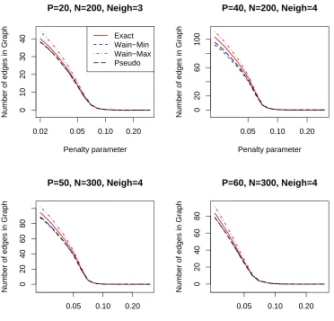
and the penalty term matrix for the pseudo-likelihood S=2R−diag(R)as defined above. For the Wainwright-methods, the penalty parameter is ρwith no penalty on the intercept. Although the log-likelihood functions that are being penalized are somewhat different, this choice of parameters makes them perform roughly equivalent, as can be seen in Figure 3. The number of edges is plotted against the penalty parameter used and all methods behave very similar. However, in order not to confound some results by these slight differences of the effects of the penalty, all the following plots are with respect to the number of edges in the graph, not the penalty parameter itself.
5.2 Speed Comparison
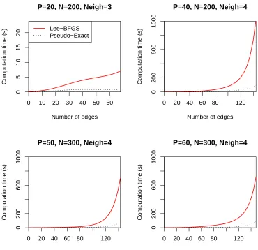
First, we compare the speed of the four methods for the L1-penalized model. We used an an-nealing schedule for Lee, Ganapathi, and Koller (2006a) to improve convergence as suggested in their article. Plots of the speeds of the exact methods can be seen in Figure 4 and the approxi-mate methods are shown in Figure 5. Each plot shows the time the algorithm needed to converge versus the number of edges in the estimated graph. As can be seen, the pseudo-likelihood based exact algorithm described above is considerable faster than the one proposed in Lee, Ganapathi, and Koller (2006a). For the approximate algorithms, we can see that the p logistic regressions in the Wainwright et al. (2006) algorithm take roughly the same amount of time as the pseudo-likelihood algorithm presented above. This is not surprising due to the similarity of the optimization methods and any difference that can be observed in Figure 5 is mostly due to the specific implementations used. Furthermore, we would like to note that we decided to plot the speed against the number of edges in the graph instead of the penalty parameter, as the runtime of the algorithm is very closely related to the actual sparseness of the graph.
0.02 0.05 0.10 0.20
0
10
20
30
40
P=20, N=200, Neigh=3
Penalty parameter
Number of edges in Graph
Exact Wain−Min Wain−Max Pseudo
0.05 0.10 0.20
0
20
60
100
P=40, N=200, Neigh=4
Penalty parameter
Number of edges in Graph
0.05 0.10 0.20
0
20
40
60
80
P=50, N=300, Neigh=4
Penalty parameter
Number of edges in Graph
0.05 0.10 0.20
0
20
40
60
80
P=60, N=300, Neigh=4
Penalty parameter
Number of edges in Graph
Figure 3: Number of edges in the graph vs. penalty parameter for different problem sizes, averaged over 20 simulations.
superior speed of the pseudo-likelihood and Wainwright et al. (2006) algorithm warrants a closer look at the trade-off with respect to accuracy.
5.3 Accuracy Comparisons
0 10 20 30 40 50 60
0
5
10
15
20
P=20, N=200, Neigh=3
Number of edges
Computation time (s)
Lee−BFGS Pseudo−Exact
0 20 40 60 80 120
0
200
600
1000
P=40, N=200, Neigh=4
Number of edges
Computation time (s)
0 20 40 60 80 120
0
200
600
1000
P=50, N=300, Neigh=4
Number of edges
Computation time (s)
0 20 40 60 80 120
0
200
600
1000
P=60, N=300, Neigh=4
Number of edges
Computation time (s)
Figure 4: Computation time of the exact algorithms versus the number of non-zero elements inΘ. Values are averages over 20 simulation runs, along with±2 standard error curves. Also, p is the number of variables in the model, N the number of observations and Neigh is the average number of neighbors per node in the simulated data. Here, Pseudo-Exact refers to the the exact solution algorithm that uses adjusted pseudo-likelihoods as presented in Section 4.
0 10 20 30 40 50 60
0.0
0.4
0.8
1.2
P=20, N=200, Neigh=3
Number of edges
Computation time (s)
Wainwright Pseudo
0 20 40 60 80 120
0.0
1.0
2.0
P=40, N=200, Neigh=4
Number of edges
Computation time (s)
0 50 100 150
0.0
1.0
2.0
3.0
P=50, N=300, Neigh=4
Number of edges
Computation time (s)
0 50 100 150 200 250
0
1
2
3
4
P=60, N=300, Neigh=4
Number of edges
Computation time (s)
Figure 5: Computation time for the approximate algorithms versus the number of non-zero ele-ments inΘ. Values are averages over 20 simulation runs, along with±2 standard error curves. Also, p is the number of variables in the model, N the number of observations and Neigh is the average number of neighbors per node in the simulated data.
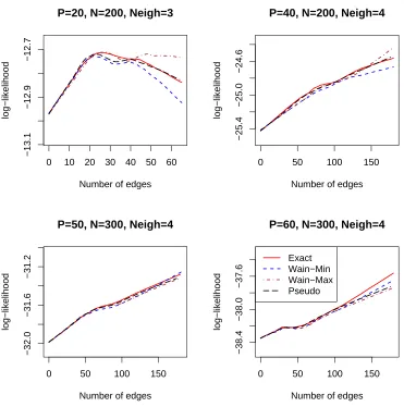
Apart from the accuracy of edge identification, we also consider other statistics. The unpenal-ized log-likelihood is a measure of how well the estimated model fits the observed data (higher values are better). Again, the approximate solutions are all very close to the exact solution (see Figure 7) and the differences are always smaller than 2 standard deviations. In Figure 8, we plot the difference of the log-likelihood with respect to the exact solution. Also in this plot, no clear ”winner” can be identified.
We also use the Kullback-Leibler divergence DKL(P||Q), which is a measure of difference
0.00 0.05 0.10 0.15 0.20 0.25
0.0
0.2
0.4
0.6
0.8
1.0
P=20, N=200, Neigh=3
False positive rate
True positive rate
Exact Wain−Min Wain−Max Pseudo
0.00 0.05 0.10 0.15
0.0
0.2
0.4
0.6
0.8
1.0
P=40, N=200, Neigh=4
False positive rate
True positive rate
0.00 0.04 0.08
0.0
0.2
0.4
0.6
0.8
1.0
P=50, N=300, Neigh=4
False positive rate
True positive rate
0.00 0.02 0.04 0.06
0.0
0.2
0.4
0.6
0.8
1.0
P=60, N=300, Neigh=4
False positive rate
True positive rate
Figure 6: ROC curves: false positive versus true positive rate for edge identification. Values are averages over 20 simulation runs.
probability distribution we use the distribution of the binary Markov network using the true Θ0 -matrix that was used to generate the simulated data. The distributionQin our case is the binary Markov network using the estimated ˆΘ-matrix. We can compute DKL(P||Q)as
DKL(P||Q) =
∑
xP(x)logP(x)
Q(x) =Ψ(Θ0)−Ψ(Θˆ) +
∑
x P(x)tr xxT(Θˆ −Θ
0)
=
=Ψ(Θ0)−Ψ(Θˆ) +tr EP(xxT)(Θˆ −Θ0) .
If the distributionsPandQare identical, then DKL(P||Q) =0. In our simulations, the exact solution
0 10 20 30 40 50 60
−13.1
−12.9
−12.7
P=20, N=200, Neigh=3
Number of edges
log−likelihood
0 50 100 150
−25.4
−25.0
−24.6
P=40, N=200, Neigh=4
Number of edges
log−likelihood
0 50 100 150
−32.0
−31.6
−31.2
P=50, N=300, Neigh=4
Number of edges
log−likelihood
0 50 100 150
−38.4
−38.0
−37.6
P=60, N=300, Neigh=4
Number of edges
log−likelihood
Exact Wain−Min Wain−Max Pseudo
Figure 7: Log-likelihood of the estimated model vs number of edges in the graph for different problem sizes, averaged over 20 simulations.
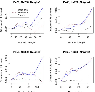
methods match the exact solution very closely and any differences are well within the 2 standard deviation error band. In Figure 10 the differences of the KL-divergence of the approximate to the exact method can be seen. Again, all methods are very close with the pseudo-likelihood approach performing the best in this case.
6. Discussion
0 10 20 30 40 50 60
−0.05
0.05
0.10
P=20, N=200, Neigh=3
Number of edges
Difference of ll to exact
Wain−Min Wain−Max Pseudo
0 50 100 150
−0.10
0.00
0.10
P=40, N=200, Neigh=4
Number of edges
Difference of ll to exact
0 50 100 150
−0.04
−0.02
0.00
0.02
P=50, N=300, Neigh=4
Number of edges
Difference of ll to exact
0 50 100 150
−0.15
−0.05
P=60, N=300, Neigh=4
Number of edges
Difference of ll to exact
Figure 8: Difference of log-likelihood of the estimated model to the exact model vs number of edges in the graph for different problem sizes, averaged over 20 simulations.
we also learned something surprising: several approximate methods exist that are much faster and only slightly less accurate than the exact methods. In addition, when a dense solution is required, the exact methods become infeasible while the approximate methods can still be used. Our imple-mentation of the methods of Wainwright et al. (2006) uses the fast coordinate descent procedure of Friedman, Hastie, and Tibshirani (2008b), a key to its speed. The pseudo-likelihood algorithm also uses similar techniques, which make it very fast as well. We conclude that the Wainwright and pseudo-likelihood methods should be seriously considered for computation in Markov networks.
0 10 20 30 40 50 60
0.18
0.22
0.26
P=20, N=200, Neigh=3
Number of edges
KL−divergence
0 50 100 150
0.48
0.52
0.56
P=40, N=200, Neigh=4
Number of edges
KL−divergence
0 50 100 150
0.50
0.60
0.70
P=50, N=300, Neigh=4
Number of edges
KL−divergence
0 50 100 150
0.65
0.75
0.85
P=60, N=300, Neigh=4
Number of edges
KL−divergence
Exact Wain−Min Wain−Max Pseudo
Figure 9: Kullback-Leibler divergence of the estimated model vs. number of edges in the graph for different problem sizes, averaged over 20 simulations.
also be possible to generalize the graph structure by introducing higher order interaction terms. Apart from these extensions, an interesting possibility for future work would also be to prove the theoretical results of Wainwright et al. (2006) for the pseudo-likelihood model. Furthermore, we believe that both the exact and fast approximate methods can also be applied to the learning of multilayer generative models, such as restricted Boltzmann machines (see Hinton, 2007).
0 10 20 30 40 50 60
0.000
0.010
P=20, N=200, Neigh=3
Number of edges
Difference of KL to exact
Wain−Min Wain−Max Pseudo
0 50 100 150
0.000
0.015
0.030
P=40, N=200, Neigh=4
Number of edges
Difference of KL to exact
0 50 100 150
0.000
0.010
0.020
P=50, N=300, Neigh=4
Number of edges
Difference of KL to exact
0 50 100 150
0.000
0.006
0.012
P=60, N=300, Neigh=4
Number of edges
Difference of KL to exact
Acknowledgments
Hoefling was supported by a Stanford Graduate Fellowship. Tibshirani was partially supported by National Science Foundation Grant DMS-9971405 and National Institutes of Health Contract N01-HV-28183. We would like to thank Trevor Hastie and Jerome Friedman for code implementing the fast L1logistic regression and Daniela Witten for helpful comments on a draft of this article. We also want to thank the editor and two anonymous reviewers for their work and helpful reviews.
Appendix A. Proof of Convergence for Penalized Pseudo-likelihood and Penalized Log-likelihood Algorithms
Lee, Lee, Abbeel, and Ng (2006b) gives a proof of convergence for an algorithm that solves an L1 constrained problem by quadratic approximation of the objective function. Here, we will follow this proof very closely and make few changes to accommodate that we are only using a first order approximation and are working with the Lagrangian form of the L1constrained problem instead of the standard form.
Assume that g(Θ)is a strictly convex function with a global minimum that we want to mini-mize. Furthermore, let fΘ
0(Θ)be a first order approximation of g at Θ0and assume that fΘ0(Θ)
is strictly convex, has a global optimum and is jointly continuous in(Θ0,Θ). Here, by first order approximation atΘ0, we mean that fΘ0−g is twice continuously differentiable with derivative 0 at
Θ0. Assume that our algorithm works as follows: initializeΘ(0);
Set k:=0;
while not converged do
With current estimateΘ(k), define local approximation fΘ(k)(Θ)to g;
Find solutionΘ∗of fΘ(k)(Θ);
Perform backtracking line search on the line fromΘ(k)toΘ∗to findΘ(k+1); Set k:=k+1;
end
ThenΘ(k) converges to the global minimizer of g(Θ). In order to show this, we first need the following lemma:
Lemma 1 LetΘ0 be any point that is not the global optimum. Then there is an open subset SΘ0 and a constant KΘ
0 such that for everyΦ0 in SΘ0 every iteration of the algorithm starting atΦ0
will return a pointΦ1that improves the objective by at least KΘ0, that is, g(Φ1)≤g(Φ0)−KΘ0.
Proof First, let fΘ
0 be an approximation to g atΘ0with global optimumΘ1. Then set
δ= fΘ
0(Θ0)−fΘ0(Θ1)
and we know thatδ>0 as Θ0is not the global optimum. Now, there exists anε>0 such that for
Φ0∈SΘ0:={Θ:||Θ−Θ0||2<ε}the following holds:
and
|fΦ
0(Φ1)−fΘ0(Θ1)| ≤
δ
4
whereΦ1is the global minimum of fΦ0. The existence of thisεfollows from the continuity and convexity of f and g. Then
fΦ
0(Φ1)≤ fΘ0(Θ1) +
δ
4≤ fΘ0(Θ0)−
3δ 4 =
=g(Θ0)− 3δ
4 ≤g(Φ0)−
δ
2.
With step size 0<t<1 in the line search, and using the previous result, it holds that
fΦ
0(Φ0+t(Φ1−Φ0))≤(1−t)fΦ0(Φ0) +t fΦ0(Φ1)≤g(Φ0)−t
δ
2
For the next step observe that the minimizerΦ1 of fΦ0 is a continuous function ofΦ0due to the convexity of f in the second argument and the continuity in both arguments. Then, as SΘ
0 is a
compact set, there exists a compact set TΘ
0 withΦ1(Φ0)∈TΘ0 for allΦ0∈SΘ0. Thus, as fΘ0 is a
first order approximation of g atΘ0, there exists a C such that for allΘ∈TΘ0 g(Θ)≤ fΘ
0(Θ) +C||Θ−Θ0||
2 2. Therefore
g(Φ0+t(Φ1−Φ0))≤g(Φ0)−tδ 2+Ct
2||Φ
1−Φ0||22≤ ≤g(Φ0)−t
δ
2+t 2CD2
where D is the diameter of TΘ
0. Now set t
∗=min1, δ 4CD2
and thus we know that it exists aΦ∗ such that
g(Φ∗)≤g(Φ0)−t∗
δ
2+t ∗2CD2. Setting KΘ
0 =t
∗δ 2−t
∗2CD2>0 now finishes the proof.
Now, using the lemma the rest of the proof is again very similar as in Lee, Lee, Abbeel, and Ng (2006b) and we only repeat it here for completeness.
Theorem 1 The algorithm converges in a finite number of steps.
Proof Pickδ>0 arbitrary. LetΘ∗the global optimum andΘ0the starting point of the algorithm. Then there exists a compact set K such that g(Θ)>g(Θ0) for everyΘ6∈K. Define Pδ={Θ: ||Θ−Θ∗|| ≥δ} ∩K. We will show convergence by showing that the algorithm can only spend a finite number of steps in Pδ. For everyΘin Pδthere exists an open set SΘ. So
Pδ⊆ ∪Θ∈P
As Pδis compact, Heine-Borel guarantees that there is a finite set Qδsuch that
Pδ⊆ ∪Θ∈Q
δSΘ.
Furthermore, as Qδis finite, define
Cδ= min
Θ∈Qδ
KΘ.
As the lemma guarantees that every step of the algorithm inside Pδimproves the objective by at least Cδand a global optimum exists by assumption, the algorithm can at most spend a finite number of steps in Pδ. Therefore, the algorithm has to converge in a finite number of steps.
For the penalized pseudo-likelihood algorithm, by definition of the approximation it is evident that it is a first order approximation. The situation for the penalized log-likelihood algorithm is a little more complicated and it will be shown in the next section of the appendix that the proposed approximation is to first order and therefore satisfies the assumptions of the proof.
Appendix B. First Order Approximation of Log-likelihood
In Section 4, we defined a function fΘ(k) to calculate the next estimateΘ(k+1). The convergence
proof in Appendix A requires that fΘ(k) is a first order approximation of the objective l(Θ|X)−
N||R∗Θ||1. Here, we want to show that this is in fact the case. For this, we need to show that fΘ(k)−l(Θ|X) +N||R∗Θ||1is twice continuously differentiable with derivative 0 atΘ(k).
First, inserting fΘ(k) from Section 4 yields
dΘ(k) =fΘ(k)−l(Θ|X) +N||R∗Θ||1= =1
2 ˜l(Θ|X) +
∑
s>t(θst−θ (k) st )
(ˆp(Θ(k))sTX)t+ (ˆp(Θ(k))Tt X)s−2·N·wst(Θ(k))
+
+
∑
s
(θss−θ(ssk))
∑
kˆ
psk(Θ(k)) + (XTX)ss−2·N·wss(Θ(k))
!! −
−
∑
s≥t
γ(θst−θst(k))2−l(Θ|X)
which has derivative
2∂dΘ(
k)
∂θst =2(XTX)st−(ˆp(Θ)TsX)t−(ˆp(Θ)Tt X)s+ (ˆp(Θ(k))TsX)t+ (ˆp(Θ(k))tTX)s−
−2·N·wst(Θ(k))−4γ(θst−θst(k))−2(XTX)st+2·N·wst(Θ)
for s6=t and 2∂dΘ
(k)
∂θst = (XTX)ss−
∑
kˆ
psk(Θ) +
∑
kˆ
psk(Θ(k)) + (XTX)ss−2·N·wss(Θ(k))−
−4γ(θss−θ(ssk))−2(XTX)ss+2·N·wss(Θ)
References
O. Banerjee, L. El Ghaoui, and A. d’Aspremont. Model selection through sparse maximum likeli-hood estimation. Journal of Machine Learning Research, 9:485–516, 2008.
J. Besag. Statistical analysis of non-lattice data. In Proceedings of the Twenty-First National Con-ference on Artificial Intelligence (AAAI-06), volume 24, pages 179–195, 1975.
D. R. Cox and N. Reid. A note on pseudolikelihood constructed from marginal densities. Biometrika, 91:729–737, 2004.
J. Dahl, L. Vandenberghe, and V. Roychowdhury. Covariance selection for non-chordal graphs via chordal embedding. Optimization Methods and Software, 2008.
J. Friedman, T. Hastie, and R. Tibshirani. Sparse inverse covariance estimation with the graphical lasso. Biostatistics, 9:432–441, 2008a.
J. Friedman, T. Hastie, and R. Tibshirani. Regularization paths for generalized linear models via coordinate descent. Technical Report, Stanford University, 2008b. Submitted.
G. E. Hinton. Learning multiple layers of representation. Trends in Cognitive Sciences, 11:428–434, 2007.
S.-I. Lee, V. Ganapathi, and D. Koller. Efficient structure learning of Markov networks using L1 -regularization. In Advances in Neural Information Processing Systems (NIPS 2006), 2006a.
S.-I. Lee, H. Lee, P. Abbeel, and A.Y. Ng. Efficient L1regularized logistic regression. In Proceed-ings of the Twenty-First National Conference on Artificial Intelligence (AAAI-06), 2006b. B. Lindsay. Composite likelihood methods. In Contemporary Mathemtics, volume 80, pages 221–
239, 1998.
N. Meinshausen and P. B¨uhlmann. High dimensional graphs and variable selection with the lasso. Annals of Statistics, 34:1436–1462, 2006.
S. Perkins, K. Lacker, and j. Theiler. Grafting: Fast, incremental feature selection by gradient descent in function space. Journal of Machine Learning Research, 3:1333–1356, 2003.
M. J. Wainwright, P. Ravikumar, and J. Lafferty. High-dimensional graphical model selection us-ing L1-regularized logistic regression. In Advances in Neural Information Processing Systems, Vancouver, 2006.
M. J. Wainwright, P. Ravikumar, and J. Lafferty. High-dimensional graphical model selection using L1-regularized logistic regression. Technical report, University of California, Berkeley, April 2008.