Multi-Instance Learning with Any Hypothesis Class
Sivan Sabato [email protected]
Microsoft Research New England 1 Memorial Drive
Cambridge, MA
Naftali Tishby [email protected]
School of Computer Science & Engineering The Hebrew University
Jerusalem 91904, Israel
Editor: Nicolas Vayatis
Abstract
In the supervised learning setting termed Multiple-Instance Learning (MIL), the examples are bags of instances, and the bag label is a function of the labels of its instances. Typically, this function is the Boolean OR. The learner observes a sample of bags and the bag labels, but not the instance labels that determine the bag labels. The learner is then required to emit a classification rule for bags based on the sample. MIL has numerous applications, and many heuristic algorithms have been used successfully on this problem, each adapted to specific settings or applications. In this work we provide a unified theoretical analysis for MIL, which holds for any underlying hypothesis class, regardless of a specific application or problem domain. We show that the sample complexity of MIL is only poly-logarithmically dependent on the size of the bag, for any underlying hypothesis class. In addition, we introduce a new PAC-learning algorithm for MIL, which uses a regular supervised learning algorithm as an oracle. We prove that efficient PAC-learning for MIL can be generated from any efficient non-MIL supervised learning algorithm that handles one-sided error. The computational complexity of the resulting algorithm is only polynomially dependent on the bag size.
Keywords: multiple-instance learning, learning theory, sample complexity, PAC learning, super-vised classification
1. Introduction
other than Boolean OR determines bag labels based on instance labels. This function is known to the learner a-priori. We term the more general setting generalized MIL.
It is possible, in principle, to view MIL as a regular supervised classification task, where a bag is a single example, and the instances in a bag are merely part of its internal representation. Such a view, however, means that one must analyze each specific MIL problem separately, and that results and methods that apply to one MIL problem are not transferable to other MIL problems. We propose instead a generic approach to the analysis of MIL, in which the properties of a MIL problem are analyzed as a function of the properties of the matching non-MIL problem. As we show in this work, the connections between the MIL and the non-MIL properties are strong and useful. The generic approach has the advantage that it automatically extends all knowledge and methods that apply to non-MIL problems into knowledge and methods that apply to MIL, without requiring specialized analysis for each specific MIL problem. Our results are thus applicable for diverse hypothesis classes, label relationships between bags and instances, and target losses. Moreover, the generic approach allows a better theoretical understanding of the relationship, in general, between regular learning and multi-instance learning with the same hypothesis class.
The generic approach can also be helpful for the design of algorithms, since it allows deriving generic methods and approaches that hold across different settings. For instance, as we show below, a generic PAC-learning algorithm can be derived for a large class of MIL problems with different hypothesis classes. Other applications can be found in follow-up research of the results we report here, such as a generic bag-construction mechanism (Sabato et al., 2010), and learning when bags have a manifold structure (Babenko et al., 2011). As generic analysis goes, it might be possible to improve upon it in some specific cases. Identifying these cases and providing tighter analysis for them is an important topic for future work. We do show that in some important cases—most notably that of learning separating hyperplanes with classical MIL—our analysis is tight up to constants.
MIL has been used in numerous applications. In Dietterich et al. (1997) the drug design appli-cation motivates this setting. In this appliappli-cation, the goal is to predict which molecules would bind to a specific binding site. Each molecule has several possible conformations (shapes) it can take. If at least one of the conformations binds to the binding site, then the molecule is labeled positive. However, it is not possible to experimentally identify which conformation was the successful one. Thus, a molecule can be thought of as a bag of conformations, where each conformation is an in-stance in the bag representing the molecule. This application employs the hypothesis class of Axis Parallel Rectangles (APRs), and has made APRs the hypothesis class of choice in several theoret-ical works that we mention below. There are many other applications for MIL, including image classification (Maron and Ratan, 1998), web index page recommendation (Zhou et al., 2005) and text categorization (Andrews, 2007).
Previous theoretical analysis of the computational aspects of MIL has been done in two main settings. In the first setting, analyzed for instance in Auer et al. (1998), Blum and Kalai (1998) and Long and Tan (1998), it is assumed that all the instances are drawn i.i.d from a single distribution over instances, so that the instances in each bag are statistically independent. Under this indepen-dence assumption, learning from an i.i.d. sample of bags is as easy as learning from an i.i.d. sample of instances with one-sided label noise. This is stated in the following theorem.
Theorem 1 (Blum and Kalai, 1998) If a hypothesis class is PAC-learnable in polynomial time
The assumption of statistical independence of the instances in each bag is, however, very limiting, as it is irrelevant to many applications.
In the second setting one assumes that bags are drawn from an arbitrary distribution over bags, so that the instances within a bag may be statistically dependent. This is clearly much more useful in practice, since bags usually describe a complex object with internal structure, thus it is implausible to assume even approximate independence of instances in a bag. For the hypothesis class of APRs and an arbitrary distribution over bags, it is shown in Auer et al. (1998) that if there exists a PAC-learning algorithm for MIL with APRs, and this algorithm is polynomial in both the size of the bag and the dimension of the Euclidean space, then it is possible to polynomially PAC-learn DNF formulas, a problem which is solvable only if
R P
=N P
(Pitt and Valiant, 1986). In addition, if it is possible to improperly learn MIL with APRs (that is, to learn a classifier which is not itself an APR), then it is possible to improperly learn DNF formulas, a problem which has not been solved to this date for general distributions. This result implies that it is not possible to PAC-learn MIL on APRs using an algorithm which is efficient in both the bag size and the problem’s dimensionality. It does not, however, preclude the possibility of performing MIL efficiently in other cases.In practice, numerous algorithms have been proposed for MIL, each focusing on a different specialization of this problem. Almost none of these algorithms assume statistical independence of instances in a bag. Moreover, some of the algorithms explicitly exploit presumed dependences between instances in a bag. Dietterich et al. (1997) propose several heuristic algorithms for finding an APR that predicts the label of an instance and of a bag. Diverse Density (Maron and Lozano-P´erez, 1998) and EM-DD (Zhang and Goldman, 2001) employ assumptions on the structure of the bags of instances. DPBoost (Andrews and Hofmann, 2003), mi-SVM and MI-SVM (Andrews et al., 2002), and Multi-Instance Kernels (G¨artner et al., 2002) are approaches for learning MIL using margin-based objectives. Some of these methods work quite well in practice. However, no generalization guarantees have been provided for any of them.
In this work we analyze MIL and generalized MIL in a general framework, independent of a specific application, and provide results that hold for any underlying hypothesis class. We assume a fixed hypothesis class defined over instances. We then investigate the relationship between learning with respect to this hypothesis class in the classical supervised learning setting with no bags, and learning with respect to the same hypothesis class in MIL. We address both sample complexity and computational feasibility.
Our sample complexity analysis shows that for binary hypothesis and thresholded real-valued hypotheses, the distribution-free sample complexity for generalized MIL grows only logarithmically with the maximal bag size. We also provide poly-logarithmic sample complexity bounds for the case of margin learning. We further provide distribution-dependent sample complexity bounds for more general loss functions. These bound are useful when only the average bag size is bounded. The results imply generalization bounds for previously proposed algorithms for MIL. Addressing the computational feasibility of MIL, we provide a new learning algorithm with provable guarantees for a class of bag-labeling functions that includes the Boolean OR, used in classical MIL, as a special case. Given a non-MIL learning algorithm for the desired hypothesis class, which can handle one-sided errors, we improperly learn MIL with the same hypothesis class. The construction is simple to implement, and provides a computationally efficient PAC-learning of MIL, with only a polynomial dependence of the run time on the bag size.
that it is not generally possible to find a low-error classification rule for instances based on a bag sample. As a simple counter example, assume that the label of a bag is the Boolean OR of the labels of its instances, and that every bag includes both a positive instance and a negative instance. In this case all bags are labeled as positive, and it is not possible to distinguish the two types of instances by observing only bag labels.
The structure of the paper is as follows. In Section 2 the problem is formally defined and notation is introduced. In Section 3 the sample complexity of generalized MIL for binary hypotheses is analyzed. We provide a useful lemma bounding covering numbers for MIL in Section 4. In Section 5 we analyze the sample complexity of generalized MIL with real-valued functions for large-margin learning. Distribution-dependent results for binary learning and real-valued learning based on the average bag size are presented in Section 6. In Section 7 we present a PAC-learner for MIL and analyze its properties. We conclude in Section 8. The appendix includes technical proofs that have been omitted from the text. A preliminary version of this work has been published as Sabato and Tishby (2009).
2. Notations and Definitions
For a natural number k, we denote[k],{1, . . . ,k}. For a real number x, we denote[x]+=max{0,x}.
log denotes a base 2 logarithm. For two vectors x,y∈Rn,hx,yidenotes the inner product of x and y. We use the function sign :R→ {−1,+1}where sign(x) =1 if x≥0 and sign(x) =−1 otherwise. For a function f : A→B, we denote by f|Cits restriction to a set C⊆A. For a univariate function
f , denote its first and second derivatives by f′and f′′respectively.
Let
X
be the input space, also called the domain of instances. A bag is a finite ordered set of instances fromX
. Denote the set of allowed sizes for bags in a specific MIL problem by R⊆N. For any set A we denote A(R),∪n∈RAn. Thus the domain of bags with a size in R and instances fromX
isX
(R). A bag of size n is denoted by ¯x= (x[1], . . . ,x[n])where each x[j]∈X
is an instance inthe bag. We denote the number of instances in ¯x by|¯x|. For any univariate function f : A→B, we
may also use its extension to a multivariate function from sequences of elements in A to sequences of elements in B, defined by f(a[1], . . . ,a[k]) = (f(a[1]), . . . ,f(a[k])).
Let I⊆Ran allowed range for hypotheses over instances or bags. For instance, I={−1,+1} for binary hypotheses and I= [−B,B]for real-valued hypotheses with a bounded range.
H
⊆IXis a hypothesis class for instances. Every MIL problem is defined by a fixed bag-labeling function ψ: I(R)→ I that determines the bag labels given the instance labels. Formally, every instance
hypothesis h :
X
→I defines a bag hypothesis, denoted by h :X
(R)→I and defined by∀¯x∈
X
(R), h(¯x),ψ(h(x[1]), . . . ,h(x[r])).The hypothesis class for bags given
H
andψis denotedH
,{h|h∈H
}. Importantly, the identity ofψis known to the learner a-priori, thus eachψdefines a different generalized MIL problem. For instance, in classical MIL, I={−1,+1}andψis the Boolean OR.We assume the labeled bags are drawn from a fixed distribution D over
X
(R)× {−1,+1}, where each pair drawn from D constitutes a bag and its binary label. Given a range I⊆Rof possible label predictions, we define a loss functionℓ:{−1,+1} ×I→R, whereℓ(y,yˆ)is the loss incurred if the true label is y and the predicted label is ˆy. The true loss of a bag-classifier h :X
(R)→I is denoted byℓ(h,D),E(X¯,Y)
∼D[ℓ(Y,h(X¯))]. We say that a sample or a distribution are realizable by
H
if thereThe MIL learner receives a labeled sample of bags{(¯x1,y1), . . . ,(¯xm,ym)} ⊆
X
(R)× {−1,+1}drawn from Dm, and returns a classifier ˆh :
X
(R)→I. The goal of the learner is to return ˆh thathas a low lossℓ(ˆh,D)compared to the minimal loss that can be achieved with the bag hypothesis class, denoted byℓ∗(
H
,D),infh∈Hℓ(h,D). The empirical loss of a classifier for bags on a labeled sample S isℓ(h,S),E(X,Y)
∼S[ℓ(Y,h(X¯))]. For an unlabeled set of bags S={¯xi}i∈[m], we denote the
multi-set of instances in the bags of S by S∪,{xi[j]|i∈[m],j∈[|¯xi|]}. Since this is a multi-set,
any instance which repeats in several bags in S is represented the same amount of time in S∪.
2.1 Classes of Real-Valued bag-functions
In classical MIL the bag function is the Boolean OR over binary labels, that is I={−1,+1}and ψ=OR :{−1,+1}(R)→ {−1,+1}. A natural extension of the Boolean OR to a function over reals is the max function. We further consider two classes of bag functions over reals, each representing a different generalization of the max function, which conserves a different subset of its properties.
The first class we consider is the class of bag-functions that extend monotone Boolean functions. Monotone Boolean functions map Boolean vectors to {−1,+1}, such that the map is monotone-increasing in each of the inputs. The set of monotone Boolean functions is exactly the set of func-tions that can be represented by some composition of AND and OR funcfunc-tions, thus it includes the Boolean OR. The natural extension of monotone Boolean functions to real functions over real vec-tors is achieved by replacing OR with max and AND with min. Formally, we define extensions of monotone Boolean functions as follows.
Definition 2 A function fromRnintoRis an extension of an n-ary monotone Boolean function if it
belongs to the set
M
ndefined inductively as follows, where the input to a function is z∈Rn:(1)∀j∈[n], z7−→z[j]∈
M
n;(2)∀k∈N+, f1, . . . ,fk∈
M
n=⇒z7−→maxj∈[k]{fj(z)} ∈M
n;(3)∀k∈N+, f1, . . . ,fk∈
M
n=⇒z7−→minj∈[k]{fj(z)} ∈M
n.We say that a bag-function ψ:R(R)→R extends monotone Boolean functions if for all n∈R, ψ|Rn ∈
M
n.The class of extensions to Boolean functions thus generalizes the max function in a natural way. The second class of bag functions we consider generalizes the max function by noting that for bounded inputs, the max function can be seen as a variant of the infinity-normkzk∞=max|z[i]|. Another natural bag-function over reals is the average function, defined asψ(z) =1
n∑i∈[n]zi, which
can be seen as a variant of the 1-normkzk1=∑i∈[n]|z[i]|. More generally, we treat the case where
the hypotheses map into I= [−1,1], and consider the class of bag functions inspired by a p-norm, defined as follows.
Definition 3 For p∈[1,∞), the p-norm bag functionψp:[−1,+1](R)→[−1,+1]is defined by:
∀z∈Rn, ψp(z), 1
n n
∑
i=1(z[i] +1)p
!1/p
−1.
Since the inputs ofψpare in[−1,+1], we haveψp(z)≡n−1/p· kz+1kp−1 where n is the length
of z. Note that the average function is simplyψ1, andψ∞≡ kz+1k∞−1≡max. Other values of p fall between these two extremes: Due to the p-norm inequality, which states that for all p∈[1,∞)
and x∈Rn, 1
nkxk1≤n−1/pkxkp≤ kxk∞, we have that for all z∈[−1,+1]n
average≡ψ1(z)≤ψp(z)≤ψ∞(z)≡max.
Many of our results hold when the scale of the output of the bag-function is related to the scale of its inputs. Formally, we consider cases where the output of the bag-function does not change by much unless its inputs change by much. This is formalized in the following definition of a Lipschitz bag function.
Definition 4 A bag functionψ:R(R)→Ris c-Lipschitz with respect to the infinity norm for c>0
if
∀n∈R,∀a,b∈Rn, |ψ(a)−ψ(b)| ≤cka−bk∞.
The average bag-function and the max bag functions are 1-Lipschitz. Moreover, all extensions of monotone Boolean functions are 1-Lipschitz with respect to the infinity norm—this is easy to verify by induction on Definition 2. All p-norm bag functions are also 1-Lipschitz, as the following derivation shows:
|ψp(a)−ψp(b)|=n−1/p· |ka+1kp− kb+1kp| ≤n−1/p· ka−bkp≤ ka−bk∞.
Thus, our results for Lipschitz bag-functions hold in particular for the two bag-function classes we have defined here, and in specifically for the max function.
3. Binary MIL
In this section we consider binary MIL. In binary MIL we let I={−1,+1}, thus we have a binary instance hypothesis class
H
⊆ {−1,+1}X. We further let our loss be the zero-one loss, defined by ℓ0/1(y,yˆ) =1[y6=yˆ]. The distribution-free sample complexity of learning relative to a binary hypothesis class with the zero-one loss is governed by the VC-dimension of the hypothesis class (Vapnik and Chervonenkis, 1971). Thus we bound the VC-dimension ofH
as a function of the maximal possible bag size r=max R, and of the VC-dimension ofH
. We show that the VC-dimension ofH
is at most logarithmic in r, and at most linear in the VC-dimension ofH
, for any bag-labeling functionψ:{−1,+1}(R)→ {−1,+1}. It follows that the sample complexity of MIL grows only logarithmically with the size of the bag. Thus MIL is feasible even for quite large bags. In fact, based on the results we show henceforth, Sabato et al. (2010) have shown that MIL can sometimes be used to accelerate even single-instance learning. We further provide lower bounds that show that the dependence of the upper bound on r and on the VC-dimension ofH
is imperative, for a large class of Boolean bag-labeling functions. We also show a matching lower bound for the VC-dimension of classical MIL with separating hyperplanes.3.1 VC-Dimension Upper Bound
Lemma 5 For any R⊆Nand any bag functionψ:{−1,+1}(R)→ {−1,+1}, and for any hypoth-esis class
H
⊆ {−1,+1}X and a finite set of bags S⊆X
(R),
H
|S≤
H
|S∪.
Proof Let h1,h2∈
H
be bag hypotheses. There exist instance hypotheses g1,g2 ∈H
such thatgi=hi for i=1,2. Assume that h1|S6=h2|S. We show that g1|S∪6=g2|S∪, thus proving the lemma.
From the assumption it follows that g1|S6=g2|S. Thus there exists at least one bag x∈S such that g2(x)6=g2(x). Denote its size by n. We haveψ(g1(x[1]), . . . ,g1(x[n]))6=ψ(g2(x[1]), . . . ,g2(x[n])). Hence there exists a j∈[n]such that g1(x[j])6=g2(x[j]).By the definition of S∪, x[j]∈S∪. There-fore g1|S∪6=g2|S∪.
Theorem 6 Assume that
H
is a hypothesis class with a finite VC-dimension d. Let r∈N andassume that R⊆[r]. Let the bag-labeling functionψ:{−1,+1}(R)→ {−1,+1}be some Boolean function. Denote the VC-dimension of
H
by dr. We havedr≤max{16,2d log(2er)}.
Proof For a set of hypotheses
J
, denote byJ
|A the restriction of each of its members to A, so thatJ
A,{h|A|h∈J
}.Since dr is the VC-dimension ofH
, there exists a set of bags S⊆X
(R)of size drthat is shattered byH
, so that|H
|S|=2dr. By Lemma 5|H
|S| ≤ |
H
|S∪|, therefore 2dr ≤ |H
|S∪|.In addition, R⊆[r] implies |S∪| ≤rdr. By applying Sauer’s lemma (Sauer, 1972; Vapnik and
Chervonenkis, 1971) to
H
we get2dr≤ |
H
|S∪| ≤e|S∪|
d d
≤
erdr
d d
,
Where e is the base of the natural logarithm. It follows that dr≤d(log(er)−log d) +d log dr.To
provide an explicit bound for dr, we bound d log drby dividing to cases:
1. Either d log dr≤12dr, thus dr≤2d(log(er)−log d)≤2d log(er),
2. or 12dr<d log dr. In this case, (a) either dr≤16,
(b) or dr>16. In this case√dr<dr/log dr<2d, thus d log dr=2d log√dr≤2d log 2d.
Substituting in the implicit bound we get dr≤d(log(er)−log d)+2d log 2d≤2d log(2er).
3.2 VC-Dimension Lower Bounds
In this section we show lower bounds for the VC-dimension of binary MIL, indicating that the dependence on d and r in Theorem 6 is tight in two important settings.
We say that a bag-function ψ:{−1,+1}(R)→ {−1,+1} is r-sensitive if there exists a num-ber n∈R and a vector c∈ {−1,+1}n such that for at least r different numbers j
1, . . . ,jr∈[n],
ψ(c[1], . . . ,c[ji], . . . ,c[n])6=ψ(c[1], . . . ,−c[ji], . . . ,c[n]). Many commonly used Boolean functions, such as OR, AND, Parity, and all their variants that stem from negating some of the inputs, are
r-sensitive for every r∈R. Our first lower bound shows ifψis r-sensitive, the bound in Theorem 6 cannot be improved without restricting the set of considered instance hypothesis classes.
Theorem 7 Assume that the bag functionψ:{−1,+1}(R)→ {−1,+1}is r-sensitive for some r∈
N. For any natural d and any instance domain
X
with|X
| ≥rd⌊log(r)⌋, there exists a hypothesis classH
with a VC-dimension at most d, such that the VC dimension ofH
is at least d⌊log(r)⌋.Proof Sinceψ is r-sensitive, there are a vector c∈ {−1,+1}n and a set J⊆n such that|J|=r
and∀j∈J,ψ(c[1], . . . ,c[n])6=ψ(c[1], . . . ,−c[j], . . . ,c[n]). Sinceψmaps all inputs to{−1,+1}, it follows that ∀j∈J,ψ(c[1], . . . ,−c[j], . . . ,c[n]) =−ψ(c[1], . . . ,c[n]). Denote a=ψ(c[1], . . . ,c[n]). Then we have
∀j∈J,y∈ {−1,+1}, ψ(c[1], . . . ,c[j]·y, . . . ,c[n]) =a·y. (1) For simplicity of notation, we henceforth assume w.l.o.g. that n=r and J= [r].
Let S⊆
X
r be a set of d⌊log(r)⌋bags of size r, such that all the instances in all the bags aredistinct elements of
X
. Divide S into d mutually exclusive subsets, each with⌊log(r)⌋bags. Denote bag p in subset t by ¯x(p,t). We define the hypothesis classH
,{h[k1, . . . ,kd]| ∀i∈[d],ki∈[2⌊log(r)⌋]},where h[k1, . . . ,kd]is defined as follows (see illustration in Table 1): For x∈
X
which is not aninstance of any bag in S, h[k1, . . . ,kd] =−1. For x=x(p,t)[j], let b(p,n) be bit p in the binary
representation of the number n, and define
h[k1, . . . ,kd](x(p,t)[j]) = (
c[j]·a(2b(p,j−1)−1) j=kt,
c[j] j6=kt.
We now show that S is shattered by
H
, indicating that the VC-dimension ofH
is at least|S|=d⌊log(r)⌋. To complete the proof, we further show that the VC-dimension of
H
is no more than d.First, we show that S is shattered by
H
: Let{y(p,t)}p∈⌊log(r)⌋,t∈[d]be some labeling over{−1,+1}for the bags in S. For each t∈[d]let
kt,1+ ⌊log(r)⌋
∑
p=1y(p,t)+1 2 ·2
p−1.
Then by Equation (1), for all p∈[⌊log(r)⌋]and t∈[d],
h[k1, . . . ,kd](¯x(p,t)) =ψ(c[1], . . . ,c[kt]·a(2b(p,kt−1)−1), . . . ,c[r])
t p Instance label h(x(p,t)[r]) Bag label h(¯xi)
1 − − − + − − − − +
1 2 − − − + − − − − +
3 − − − − − − − − −
1 − − − − − − − + +
2 2 − − − − − − − + +
3 − − − − − − − + +
1 − − − − − − − − −
3 2 − + − − − − − − +
3 − − − − − − − − −
Table 1: An example of the hypotheses h=h[4,8,3], withψ=OR (so that c is the all−1 vector),
r=8, and d=3. Each line represents a bag in S, each column represents an instance in the bag.
Thus h[k1, . . . ,kd]labels S according to{y(p,t)}.
Second, we show that the VC-dimension of
H
is no more than d. Let A⊆X
of size d+1. If there is an element in A which is not an instance in S then this element is labeled−1 by all h∈H
, therefore A is not shattered. Otherwise, all elements in A are instances in bags in S. Since there are d subsets of S, there exist two elements in A which are instances of bags in the same subsett. Denote these instances by x(p1,t)[j1]and x(p2,t)[j2]. Consider all the possible labelings of the two elements by hypotheses in
H
. If A is shattered, there must be four possible labelings for these elements. However, by the definition of h[k1, . . . ,kd]it is easy to see that if j1= j2= j then there are at most two possible labelings by hypotheses inH
, and if j16= j2 then there are at most three possible labelings. Thus A is not shattered byH
, hence the VC-dimension ofH
is no more than d.Theorem 10 below provides a lower bound for the VC-dimension of MIL for the important case where the bag-function is the Boolean OR and the hypothesis class is the class of separating hyperplanes inRn. For w∈Rn, the function h
w:Rn→ {−1,+1}is defined by hw(x) =sign(hw,xi). The hypothesis class of linear classifiers is
W
n,{hw|w∈Rn}. Let r∈N. We denote the VC-dimension ofW
n for R={r} andψ=OR by dr,n. We prove a lower bound for dr,n using twolemmas: Lemma 8 provides a lower bound for dr,3, and Lemma 9 links dr,nfor small n with dr,nfor
large n. The resulting general lower bound, which holds for r=max R, is then stated in Theorem 10.
Lemma 8 Let dr,nbe the VC-dimension of
W
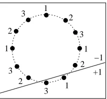
nas defined above. Then dr,3≥ ⌊log(2r)⌋.Proof Denote L,⌊log(2r)⌋. We will construct a set S of L bags of size r that is shattered by
W
3. The construction is illustrated in Figure 1.Let n= (n1, . . . ,nK)be a sequence of indices from[L], created by concatenating all the subsets of
[L]in some arbitrary order, so that K=L2L−1, and every index appears 2L−1≤r times in n. Define
a set A={ak|k∈[K]} ⊆R3 where ak,(cos(2πk/K),sin(2πk/K),1)∈R3, so that a1, . . . ,aK are
3 2 2
1
3 3
1 2
2 1
−1
+1 1
3
Figure 1: An illustration of the constructed shattered set, with r=4 and L=log 4+1=3. Each dot corresponds to an instance. The numbers next to the instances denote the bag to which an instance belongs, and match the sequence N defined in the proof. In this illustration bags 1 and 3 are labeled as positive by the bag-hypothesis represented by the solid line.
We now show that S is shattered by
W
3: Let(y1, . . . ,yL)be some binary labeling of L bags, andlet Y ={i|yi= +1}. By the definition of n, there exist j1,j2 such that Y ={nk| j1≤k≤ j2}. Clearly, there exists a hyperplane w∈R3that separates the vectors{ak|j1≤k≤ j2}from the rest of the vectors in A. Thus sign(hw,aki) = +1 if and only if j1≤k≤ j2. It follows that hw(¯xi) = +1
if and only if there is a k∈ {j1, . . . ,j2}such that akis an instance in ¯xi, that is such that nk=i. This
condition holds if and only if i∈Y , hence hwclassifies S according to the given labeling. It follows that S is shattered by
W
3, therefore dr,3≥ |S|=⌊log(2r)⌋.Lemma 9 Let k,n,r be natural number such that k≤n. Then dr,n≥ ⌊n/k⌋dr,k.
Proof For a vector x∈Rk and a number t ∈ {0, . . . ,⌊n/k⌋} define the vector s(x,t),(0, . . . ,0,
x[1], . . . ,x[k],0, . . . ,0) ∈ Rn, where x[1] is at coordinate kt+1. Similarly, for a bag ¯xi =
(xi[1], . . . ,xi[r])∈(Rk)r, define the bag s(¯xi,t),(s(xi[1],t), . . . ,s(xi[r],t))∈(Rn)r.
Let Sk={¯xi}i∈[dr,k]⊆(R
k)rbe a set of bags with instances inRkthat is shattered by
W
k. Define Sn, a set of bags with instances inRn: Sn,{s(¯xi,t)]}i∈[dr,k],t∈[⌊n/k⌋]⊆(R
n)r. Then S
n is shattered
by
W
n: Let {y(i,t)}i∈[dr,k],t∈[⌊n/k⌋] be some labeling for Sn. Sk is shattered byW
k, hence there areseparators w1, . . . ,w⌊n/k⌋∈Rk such that∀i∈[dr,k],t∈ ⌊n/k⌋, hwt(¯xi) =y(i,t).
Set w,∑⌊t=n/0k⌋s(wt,t). Thenhw,s(x,t)i=hwt,xi. Therefore
hw(s(¯xi,t)) =OR(sign(hw,s(xi[1],t)i), . . . ,sign(hw,s(xi[r],t)i))
=OR(sign(hwt,xi[1]i), . . . ,sign(hwt,xi[r]i)) =hwt(¯xi) =y(i,t). Snis thus shattered, hence dr,n≥ |Sn|=⌊n/k⌋dr,k.
The desired theorem is an immediate consequence of the two lemmas above, by noting that when-ever r∈R, the VC-dimension of
W
nis at least dr,n.Theorem 10 Let
W
nbe the class of separating hyperplanes inRnas defined above. Assume that thebag function isψ=OR and the set of allowed bag sizes is R. Let r=max R. Then the VC-dimension
3.3 Pseudo-dimension for Thresholded Functions
In this section we consider binary hypothesis classes that are generated from real-valued functions using thresholds. Let
F
⊆RX be a set of real valued functions. The binary hypothesis class of thresholded functions generated byF
is TF ={(x,z)7→sign(f(x)−z)|f∈F
,z∈R}, where x∈X
and z∈R. The sample complexity of learning with TF and the zero-one loss is governed by the pseudo-dimension of
F
, which is equal to the VC-dimension of TF (Pollard, 1984). In this section we consider a bag-labeling function ψ:R(R)→R, and bound the pseudo-dimension ofF
, thus providing an upper bound on the sample complexity of binary MIL with TF. The following bound holds for bag-labeling functions that extend monotone Boolean functions, defined in Definition 2.Theorem 11 Let
F
⊆RX be a function class with pseudo-dimension d . Let R⊆[r], and assumethatψ:R(R)→Rextends monotone Boolean functions. Let drbe the pseudo-dimension of
F
. Thendr≤max{16,2d log(2er)}.
Proof First, by Definition 2, we have that for anyψwhich extends monotone Boolean functions, any n∈R and any y∈Rn,
sign(ψ(y[1], . . . ,y[n])−z) =sign(ψ(y[1]−z, . . . ,y[n]−z))
=ψ(sign(y[1]−z, . . . ,y[n]−z)). (2)
This can be seen by noting that each of the equalities holds for each of the operations allowed by
M
nfor each n, thus by induction they hold for all functions inM
nand all combinations of them. For a real-valued function f let tf :X
×R→ {−1,+1}be defined by tf(y,z) =sign(f(y)−z).We have TF ={tf | f ∈
F
}, and TF ={tf | f ∈F
}. In addition, for all f ∈F
, z∈R, n∈R and¯x∈
X
n, we havetf(¯x,z) =sign(f(¯x)−z) =sign(ψ(f(x[1]), . . . ,f(x[n]))−z)
=ψ(sign(f(x[1])−z, . . . ,f(x[n])−z)) (3)
=ψ(tf(x[1],z), . . . ,tf(x[n],z)) =tf(¯x,z),
where the equality on line (3) follows from Equation (2). Therefore
TF ={tf | f∈
F
}={tf | f ∈F
}={h|h∈TF}=TF.The VC-dimension of TF is equal to the pseudo-dimension of
F
, which is d. Thus, by Theorem 6 and the equality above, the VC-dimension of TF is bounded by max{16,2d log(2er)}. The proof is completed by noting that dr, the pseudo-dimension ofF
, is exactly the VC-dimension of TF.4. Covering Numbers Bounds for MIL
Covering numbers are a useful measure of the complexity of a function class, since they allow bounding the sample complexity of a class in various settings, based on uniform convergence guar-antees (see, e.g., Anthony and Bartlett, 1999). In this section we provide a lemma that relates the covering numbers of bag hypothesis classes with those of the underlying instance hypothesis class. We will use this lemma in subsequent sections to derive sample complexity upper bounds for addi-tional settings of MIL. Let
F
⊆RAbe a set of real-valued functions over some domain A. Aγ-cover ofF
with respect to a normk·k◦defined on functions is a set of functionsC
⊆RAsuch that for anyf ∈
F
there exists a g∈C
such thatkf−gk◦≤γ.The covering number for givenγ>0,F
and◦, denoted byN
(γ,F
,◦), is the size of the smallest suchγ-covering forF
.Let S⊆A be a finite set. We consider coverings with respect to the Lp(S) norm for p≥1, defined by
kfkLp(S), 1
|S|s
∑
∈S|f(s)| p!1/p
.
For p=∞, L∞(S)is defined bykfkL∞(S),maxs∈S|f(S)|. The covering number of
F
for a samplesize m with respect to the Lpnorm is
N
m(γ,F
,p), sup S⊆A:|S|=mN
(γ,F
,Lp(S)).A small covering number for a function class implies faster uniform convergence rates, hence smaller sample complexity for learning. The following lemma bounds the covering number of bag hypothesis-classes whenever the bag function is Lipschitz with respect to the infinity norm (see Definition 4). Recall that all extensions of monotone Boolean functions (Definition 2) and all p-norm bag-functions (Definition 3) are 1-Lipschitz, thus the following lemma holds for them with
a=1.
Lemma 12 Let R⊆Nand suppose the bag functionψ:R(R)→Ris a-Lipschitz with respect to the
infinity norm, for some a>0. Let S⊆
X
(R)be a finite set of bags, and let r be the average size of a bag in S. For anyγ>0, p∈[1,∞], and hypothesis classH
⊆RX,N
(γ,H
,Lp(S))≤N
( γar1/p,
H
,Lp(S∪)).
Proof First, note that by the Lipschitz condition on ψ, for any bag ¯x of size n and hypotheses
h,g∈
H
,|h(¯x)−g(¯x)|=|ψ(h(x[1]), . . . ,h(x[n]))−ψ(g(x[1]), . . .,g(x[n]))| ≤a max
Then by Equation (4)
kh−gkLp(S)= 1
|S|¯x
∑
∈S|h(¯x)−g(¯x)| p!1/p
≤ a
p
|S|¯x
∑
∈Smaxx∈¯x |h(x)−g(x)|p !1/p
≤ a
p
|S|¯x
∑
∈Sx∑
∈¯x|h(x)−g(x)| p!1/p
= a
|S|1/p
∑
x∈S∪|h(x)−g(x)|p
!1/p
=a
|S∪|
|S| 1/p
1
|S∪|x
∑
∈S∪|h(x)−g(x)|p !1/p
=ar1/pkh−gkLp(S∪)≤ar 1/p·γ.
It follows that
C
is a(ar1/pγ)-covering forH
. For p=∞we havekh−gkL∞(S)=max
¯x∈S |h(¯x)−g(¯x)| ≤a max¯x∈S maxx∈¯x |h(x)−g(x)| =a max
x∈S∪|h(x)−g(x)|=akh−gkL∞(S∪)≤aγ=a·r
1/p
·γ.
Thus in both cases,
C
is a ar1/pγ-covering forH
, and its size isN
(γ,H
,Lp(S∪)). ThusN
(ar1/pγ,H
,Lp(S∪))≤N
(γ,H
,Lp(S∪)). We get the statement of the lemma by substitutingγwith γar1/p.
As an immediate corollary, we have the following bound for covering numbers of a given sample size.
Corollary 13 Let r∈N, and let R⊆[r]. Suppose the bag functionψ:R(R)→Ris a-Lipschitz with
respect to the infinity norm for some a>0. Letγ>0,p∈[1,∞], and
H
∈RX. For any m≥0,N
m(γ,H
,p)≤N
rm( γa·r1/p,
H
,p).5. Margin Learning for MIL: Fat-Shattering Dimension
of MIL as a function of the fat-shattering dimension of the underlying hypothesis class, and of the maximal allowed bag size. The bound holds for any Lipschitz bag-function. Letγ>0 be the desired margin. For a hypothesis class H, denote itsγ-fat-shattering dimension by Fat(γ,H)
Theorem 14 Let r∈Nand assume R⊆[r]. Let B,a>0. Let
H
⊆[0,B]X be a real-valuedhypoth-esis class and assume that the bag functionψ:[0,B](R)→[0,aB]is a-lipschitz with respect to the infinity norm. Then for allγ∈(0,aB]
Fat(γ,
H
)≤max33,24Fat( γ
64a,
H
)log 2
6·2048·B2a2
γ2 ·Fat( γ
64a,
H
)·r. (5)
This theorem shows that for margin learning as well, the dependence of the bag size on the sample complexity is poly-logarithmic. In the proof of the theorem we use the following two results, which link the covering number of a function class with its fat-shattering dimension.
Theorem 15 (Bartlett et al., 1997) Let F be a set of real-valued functions and letγ>0. For m≥
Fat(16γ,F),
eFat(16γ,F)/8≤
N
m(γ,F,∞).The following theorem is due to Anthony and Bartlett (1999) (Theorem 12.8), following Alon et al. (1993).
Theorem 16 Let F be a set of real-valued functions with range in[0,B]. Letγ>0. For all m≥1,
N
m(γ,F,∞)<24B2m γ2
Fat(γ4,F)log(4eBm/γ)
. (6)
Theorem 12.8 in Anthony and Bartlett (1999) deals with the case m≥Fat(γ4,F). Here we only require m≥1, since if m≤Fat(4γ)then the trivial upper bound
N
m(γ,H
,∞)≤(B/γ)m≤(B/γ)Fat(γ
4)
implies Equation (6).
Proof [of Theorem 14] From Theorem 15 and Lemma 12 it follows that for m≥Fat(16γ,
H
), Fat(16γ,H
)≤ 8log elog
N
m(γ,H
,∞)≤6 logN
rm(γ/a,H
,∞). (7) By Theorem 16, for all m≥1, if Fat(γ/4)≥1 then∀γ≤ B
2e, log
N
m(γ,H
,∞)≤1+Fat( γ4,
H
)log( 4eBmγ )log
4B2m
γ2
≤Fat(γ
4,
H
)log( 8eBmγ )log
4B2m
γ2
(8)
≤Fat(γ
4,
H
)log2(4B2m
γ2 ). (9) The inequality in line (8) holds since we have added 1 to the second factor, and the value of the other factors is at least 1. The last inequality follows since ifγ≤ 2eB, we have 8eB/γ≤4B2/γ2. Equa-tion (9) also holds if Fat(γ/4)<1, since this implies Fat(γ/4) =0 and
N
m(γ,H
,∞) =1. Combining Equation (7) and Equation (9), we get that if m≥Fat(16γ,H
)then∀γ≤aB2e, Fat(16γ,
H
)≤6Fat( γ4a,
H
)log2(4B2a2rm
Set m=⌈Fat(16γ,
H
)⌉ ≤Fat(16γ,H
) +1. If Fat(16γ,H
)≥1, we have that m≥Fat(16γ,H
)and also m≤2Fat(16γ,H
). Thus Equation (10) holds, and∀γ≤aB2e, Fat(16γ,
H
)≤6Fat( γ4a,
H
)log2(4B2a2
γ2 ·r·(Fat(16γ,
H
) +1)) ≤6Fat( γ4a,
H
)log2(8B2a2
γ2 ·r·Fat(16γ,
H
)).Now, it is easy to see that if Fat(16γ,
H
)<1, this inequality also holds. Therefore it holds in general. Substitutingγwithγ/16, we have that∀γ≤8aB
e , Fat(γ,
H
)≤6Fat(γ
64a,
H
)log2(2048B2a2
γ2 ·r·Fat(γ,
H
)). (11) Note that the condition onγholds, in particular, for allγ≤aB.To derive the desired Equation (5) from Equation (11), let β =6Fat(γ/64a,
H
) and η=2048B2a2/γ2. Denote F =Fat(γ,
H
). Then Equation (11) can be restated as F ≤βlog2(ηrF). It follows that√F/log(ηrF)≤pβ, Thus
√
F
log(ηrF)log
√η rF
log(ηrF)
≤pβlog(pβηr).
Therefore √
F
log(ηrF)(log(ηrF)/2−log(log(ηrF)))≤
p
βlog(βηr)/2,
hence
(1−2 log(log(ηrF)) log(ηrF) )
√
F≤pβlog(βηr).
Now, it is easy to verify that log(log(x))/log(x)≤1
4 for all x≥33·2048. Assume F≥33 and γ≤aB. Then
ηrF=2048B2a2rF/γ2≥2048F≥33·2048.
Therefore log(log(ηrF))/log(ηrF) ≤ 14, which implies 12√F ≤ pβlog(βηr). Thus F ≤ 4βlog2(βηr). Substituting the parameters with their values, we get the desired bound, stated in Equation (5).
6. Sample Complexity by Average Bag Size: Rademacher Complexity
The upper bounds we have shown so far provide distribution-free sample complexity bounds, which depend only on the maximal possible bag size. In this section we show that even if the bag size is unbounded, we can still have a sample complexity guarantee, if the average bag size for the input distribution is bounded. For this analysis we use the notion of Rademacher complexity (Bartlett and Mendelson, 2002). Let A be some domain. The empirical Rademacher complexity of a class of functions
F
⊆RA×{−1,+1}with respect to a sample S={(xi,yi)}i∈[m]⊆A× {−1,+1}isR
(F
,S), 1mEσ[|supf∈Fi∈
∑
[m]whereσ= (σ1, . . . ,σm)are m independent uniform{±1}-valued variables. The average Rademacher
complexity of
F
with respect to a distribution D over A× {−1,+1}and a sample size m isR
m(F
,D),ES∼Dm[R
(F
,S)].The worst-case Rademacher complexity over samples of size m is
R
msup(F
) = supS⊆Am
R
(F
,S).This quantity can be tied to the fat-shattering dimension via the following result:
Theorem 17 (See, for example, Mendelson, 2002, Theorem 4.11) Let m ≥ 1 and γ ≥ 0.
If
R
msup(F
)≤γthen theγ-fat-shattering dimension ofF
is at most m.Let I⊆R. Assume a hypothesis class H ⊆IA and a loss functionℓ:{−1,+1} ×I→R. For a hypothesis h∈H, we denote by hℓthe function defined by hℓ(x,y) =ℓ(y,h(x)). Given H andℓ, we
define the function class Hℓ,{hℓ|h∈H} ⊆RA×{−1,+1}.
Rademacher complexities can be used to derive sample complexity bounds (Bartlett and Mendel-son, 2002): Assume the range of the loss function is[0,1]. For anyδ∈(0,1), with probability of 1−δover the draw of samples S⊆A× {−1,+1}of size m drawn from D, every h∈H satisfies
ℓ(h,D)≤ℓ(h,S) +2
R
m(Hℓ,D) +r
8 ln(2/δ)
m . (12)
Thus, an upper bound on the Rademacher complexity implies an upper bound on the average loss of a classifier learned from a random sample.
6.1 Binary MIL
Our first result complements the distribution-free sample complexity bounds that were provided for binary MIL in Section 3. The average (or expected) bag size under a distribution D over
X
(R)×{−1,+1}isE
(X¯,Y)∼D[|X¯|]. Our sample complexity bound for binary MIL depends on the average bag size and the VC dimension of the instance hypothesis class. Recall that the zero-one loss is defined byℓ0/1(y,yˆ) =1[y6=yˆ]. For a sample of labeled examples S={(xi,yi)}i∈[m], we use SX to
denote the examples of S, that is SX ={xi}i∈[m].
Theorem 18 Let
H
⊆ {−1,+1}X be a binary hypothesis class with VC-dimension d. Let R⊆Nand assume a bag function ψ:{−1,+1}(R)→ {−1,+1}. Let r be the average bag size under distribution D over labeled bags. Then
R
(H
ℓ0/1,D)≤17 rd ln(4er)
m .
Proof Let S be a labeled bag-sample of size m. Dudley’s entropy integral (Dudley, 1967) states that
R
(H
ℓ0/1,S)≤√12m
Z ∞
0
q
ln
N
(γ,H
ℓ0/1,L2(S))dγ (13) =√12m
Z 1 0
q
The second equality holds since for anyγ>1,
N
(γ,H
ℓ0/1,L2(S)) =1, thus the expression in the integral is zero.If
C
is aγ-cover forH
with respect to the norm L2(SX), thenC
ℓ0/1 is aγ/2-cover forH
ℓ0/1 withrespect to the norm L2(S). This can be seen as follows: Let hℓ0/1∈
H
ℓ0/1 for some h∈H
. Let f∈C
such thatkf−hkL2(SX)≤γ. We have
kfℓ0/1−hℓ0/1kL2(S)=
1
m(x,
∑
y)∈S|fℓ0/1(x,y)−hℓ0/1(x,y)|2
!1/2
= 1
m(x,
∑
y)∈S
|ℓ0/1(y,f(x))−ℓ0/1(y,h(x))|2
!1/2
= 1
mx
∑
∈SX (1
2|f(x)−h(x)|) 2
!1/2
=1
2kf−hkL2(SX)≤γ/2.
Therefore
C
ℓ0/1 is aγ/2-cover for L2(S). It follows that we can bound theγ-covering number ofH
ℓ0/1 by:N
(γ,H
ℓ0/1,L2(S))≤N
(2γ,H
,L2(SX)). (14) Let r(S)be the average bag size in the sample S, that is r(S) =|S∪|/|S|. By Lemma 12,N
(γ,H
,L2(SX))≤N
(γ/p
r(S),
H
,L2(S∪X)). (15)From Equation (13), Equation (14) and Equation (15) we conclude that
R
(H
ℓ0/1,S)≤ √12m
Z 1 0
q
ln
N
(2γ/pr(S),H
,L2(S∪X))dγ.By Dudley (1978), for any
H
with VC-dimension d, and anyγ>0,ln
N
(γ,H
,L2(S∪X))≤2d ln 4e γ2 . ThereforeR
(H
ℓ0/1,S)≤√12m Z 1 0 s 2d ln
er(S) γ2 dγ ≤17 r d m Z 1 0 p
ln(er(S))dγ+
Z 1 0
q
ln(1/γ2)dγ
=17 s
d(ln(er(S)) +pπ/2)
m ≤17
r
d ln(4er(S))
m .
The functionpln(x)is concave for x≥1. Therefore we may take the expectation of both sides of this inequality and apply Jensen’s inequality, to get
R
m(H
ℓ0/1,D) =ES∼Dm[R
(H
ℓ0/1,S)]≤ES∼Dm"
17 r
d ln(4er(S))
m #
≤17 r
d ln(4e·ES∼Dm[r(S)])
m =17
r
d ln(4er)
We conclude that even when the bag size is not bounded, the sample complexity of binary MIL with a specific distribution depends only logarithmically on the average bag size in this distribution, and linearly on the VC-dimension of the underlying instance hypothesis class.
6.2 Real-Valued Hypothesis Classes
In our second result we wish to bound the sample complexity of MIL when using other loss functions that accept real valued predictions. This bound will depend on the average bag size, and on the Rademacher complexity of the instance hypothesis class.
We consider the case where both the bag function and the loss function are Lipschitz. For the bag function, recall that all extensions of monotone Boolean functions are Lipschitz with respect to the infinity norm. For the loss functionℓ:{−1,+1} ×R→R, we require that it is Lipschitz in its second argument, that is, that there is a constant a>0 such that for all y∈ {−1,+1}and
y1,y2∈R,|ℓ(y,y1)−ℓ(y,y2)| ≤a|y1−y2|. This property is satisfied by many popular losses. For instance, consider the hinge-loss, which is the loss minimized by soft-margin SVM. It is defined as ℓhl(y,yˆ) = [1−y ˆy]+, and is 1-Lipschitz in its second argument.
The following lemma provides a bound on the empirical Rademacher complexity of MIL, as a function of the average bag size in the sample and of the behavior of the worst-case Rademacher complexity over instances. We will subsequently use this bound to bound the average Rademacher complexity of MIL with respect to a distribution. We consider losses with the range[0,1]. To avoid degenerate cases, we consider only losses such that there exists at least one labeled bag(¯x,y)⊆
X
(R)× {−1,+1}and hypotheses h,g∈H
such that hℓ(¯x,y) =0 and gℓ(¯x,y) =1. We say that such
a loss has a full range.
Lemma 19 Let
H
⊆[0,B]X be a hypothesis class. Let R⊆N, and let the bag functionψ:R(R)→Rbe a1-Lipschitz with respect to the infinity norm. Assume a loss functionℓ:{−1,+1} ×R→[0,1],
which is a2-Lipschitz in its second argument. Further assume thatℓhas a full range. Suppose there
is a continuous decreasing function f :(0,1]→Rsuch that
∀γ∈(0,1], f(γ)∈N=⇒
R
fsup(γ)(H
)≤γ.Let S be a labeled bag-sample of size m, with an average bag size r. Then for allε∈(0,1],
R
(H
ℓ,S)≤4ε+√10mlog
4ea21a22B2rm
ε2 1+ Z 1
ε
r f( γ
4a1a2 )dγ
.
Proof A refinement of Dudley’s entropy integral (Srebro et al., 2010, Lemma A.3) states that for allε∈(0,1], for all real function classes
F
with range[0,1]and for all sets S,R
(F
,S)≤4ε+√10m
Z 1
ε
q
ln
N
(γ,F
,L2(S))dγ. (16) Since the range ofℓis[0,1], this holds forF
=H
ℓ. In addition, for any set S, the L2(S) norm is bounded from above by the L∞(S)norm. ThereforeN
(γ,F
,L2(S))≤N
(γ,F
,L∞(S)). Thus, by Equation (16) we haveR
(H
ℓ,S)≤4ε+√10m
Z 1
ε
q
![Table 1: An example of the hypotheses h = h[4,8,3], with ψ = OR (so that c is the all −1 vector),r = 8, and d = 3](https://thumb-us.123doks.com/thumbv2/123dok_us/9819918.1967893/9.612.165.448.89.232/table-example-hypotheses-h-h-ps-c-vector.webp)