Feature Extraction by Non-Parametric Mutual Information
Maximization
Kari Torkkola [email protected]
Motorola Labs
7700 South River Parkway, MD ML28 Tempe AZ 85284, USA
Editors: Isabelle Guyon and Andr´e Elisseeff
Abstract
We present a method for learning discriminative feature transforms using as criterion the mutual information between class labels and transformed features. Instead of a commonly used mutual in-formation measure based on Kullback-Leibler divergence, we use a quadratic divergence measure, which allows us to make an efficient non-parametric implementation and requires no prior assump-tions about class densities. In addition to linear transforms, we also discuss nonlinear transforms that are implemented as radial basis function networks. Extensions to reduce the computational complexity are also presented, and a comparison to greedy feature selection is made.
Keywords: Mutual information, Renyi entropy, Quadratic divergence measures, Parzen
estima-tion, Feature transform, Feature extracestima-tion, Non-parametric estimation
1. Introduction
Reducing the dimensionality of the raw input variable space is an important step in pattern recog-nition tasks often dictated by practical feasibility. Dimensionality reduction is also essential in exploratory data analysis, where the purpose is to map data onto a low-dimensional space for im-proved visualization. We are interested in methods that reveal or enhance the class structure of the data. This is an important step in the process of selecting or designing appropriate classifiers for a given domain. Usually this is done by using domain knowledge, heuristics, or traditions in the field. But optimally, we would like to use class discrimination as the criterion.
There are two major categories of methods of dimensionality reduction. Feature selection meth-ods keep only useful features and discards others. Feature transform methmeth-ods construct new fea-tures out of the original variables.1 In pattern recognition, optimal feature selection coupled with a particular classifier can be done by training and evaluating the classifier using all combinations of available features. However, this wrapper strategy leads to a combinatorial computational problem and it does not lend itself to learning feature transforms, because all possible transforms cannot be enumerated and compared. In contrast, the filter strategy is to discover features, subset of features or feature transforms by evaluating some criterion. Filter based greedy algorithms using the sequen-tial selection of the feature having the best criterion value are computationally more efficient than wrappers. However, in application to feature selection this strategy has also its limitations, as it fails to find a feature set that would jointly maximize the criterion (Koller and Sahami, 1996).
For this very reason, finding a transform to lower dimensions might be easier than selecting features, given an appropriate criterion that measures the joint “importance” of a set of features. If the criterion is differentiable with respect to the parameters of the transform, and if the transform is smooth, then it is possible to learn the transform by optimizing the criterion. In contrast, feature selection is not a smooth process, since switching from a feature to another is a discrete event, and thus cannot be learned by a similar numerical optimization process.2 A further motivation for trans-forms is the ability to extract distributed relevant information across several original features, which produces a more compact representation than selection. However, feature selection is preferable to transforms if it is essential to retain some of the original features. In addition, when the number of irrelevant features exceeds the number of relevant features by orders of magnitude, learning a transform reliably may require excessive amounts of training data. We return to this issue later.
One well known linear transform for dimensionality reduction is principal component analysis or PCA (Devijver and Kittler, 1982). The transform is derived from eigenvectors corresponding to the largest eigenvalues of the covariance matrix for data of all classes. PCA seeks to optimally rep-resent the data in terms of minimal mean-square-error between the reprep-resentation and the original data. Thus PCA has little to do with discriminative features optimal for classification. However, it may be very useful in reducing noise in the data by separating signal and noise subspaces. Kernel methods have recently provided means to implement PCA in a nonlinear fashion in the form of kernel-PCA (Scholkopf et al., 1998).
Linear discriminant analysis3 (LDA) produces a transform that is optimally discriminative for certain cases (Fukunaga, 1990). LDA finds eigenvectors of T=S−w1Sb, where Sb is the between-class covariance matrix, and Swis the sum of within-class covariance matrices. Matrix S−w1captures the compactness of each class, and Sb represents the separation of the class means. Eigenvectors corresponding to the largest eigenvalues of T form columns of the transform matrix W, and new discriminative features y are derived from the original features x by y=WTx. Since LDA only
makes use of second-order statistical information, the covariances, it is optimal for data where each class has a unimodal Gaussian density with well separated means. Furthermore, the maximum rank of Sb is Nc−1, where Ncis the number of different classes. Thus LDA cannot produce more than
Nc−1 features. Although extensions have been proposed for the latter problem (see Okada and Tomita, 1985), the first one remains.
Independent component analysis (ICA) has also been proposed as a tool to find “interesting” projections of the data (Girolami et al., 1998, Yang and Moody, 2000). Girolami et al. (1998) maximize negentropy (divergence to a Gaussian density function) to find a subspace on which the data has the least Gaussian projection. The criterion corresponds to finding a projection of data that looks maximally clustered. This appears to be a very useful tool for revealing non-Gaussian structures in the data. However, like PCA, the method is completely unsupervised with regard to the class labels of the data, and it is not able to enhance class separability.
An optimal criterion for classification would naturally reflect the Bayes error rate in the trans-formed space, which can be written as
E(Y) =
y
p(y)
1−max
i (p(ci|y))
dy ,
2. Weston et al. (2001) present an approach for this using approximate integer programming combined with Support Vector Machines.
where y denotes the feature vector in the transformed space and ci denotes the class label. This criterion requires models of posterior probability density functions of classes, and numerical inte-gration of those, which is difficult in practice given only a training data set. It is possible to use approximations of the error rate based on Bhattacharyya bound or on an interclass divergence cri-terion (Devijver and Kittler, 1982, Guorong et al., 1996, Saon and Padmanabhan, 2001). These approximations make use of class-conditional density functions, and they must be accompanied by a parametric estimation of the densities followed by numerical optimization of the approxima-tion. Gaussian assumption usually needs to be made about the class-conditional densities to make optimization tractable.4
As mentioned, LDA assumes all classes to be Gaussian with a single shared covariance matrix. Heteroscedastic Discriminant Analysis (HDA) extends this by allowing each of the classes have their own covariances with the expense of resorting to numerical multivariate optimization to find the transform (Kumar and Andreou, 1998). Thus HDA resembles methods that assume parametric densities and optimize divergence measures of those.
What this paper attempts to show is that mutual information (MI) between the class labels and the transformed data acts as a more general criterion that overcomes many limitations of the methods discussed above. MI accounts for higher-order statistics, not just for second order. In addition, it can also be used as the basis for non-linear transforms. MI also bounds the optimal Bayes error rate (Fano, 1961, Hellman and Raviv, 1970). The reasons why mutual information is not in wider use currently (except between two scalar variables) lie in computational difficulties. The probability density functions of the variables are required, and MI involves numerical integration of functions of those, which leads to a high computational complexity.
Evaluating MI between two scalar variables is feasible through histograms. This approach has found use in feature selection rather than in feature transform (Battiti, 1994, Bonnlander and Weigend, 1994, Yang and Moody, 2000). As with any criterion, greedy sequential feature selection using MI is not optimal since it is the joint MI between features and class labels that should be maximized. Yang and Moody (2000) visualize data by selecting those two features of all N2 com-binations that maximize the joint MI of the two features and labels. This is barely feasible for two features but not for more. Bollacker and Ghosh (1996) proceed sequentially to find a linear trans-form. They find a single direction that maximizes the MI between the classes and that direction. They then continue in a subspace orthogonal to the previously found directions.
While histogram-based MI estimation works with two or even three variables, it fails in higher dimensions. This failure is due to the sparsity of (any amount of) data in high-dimensional spaces for histogram-based estimation. As a heuristic solution, Bollacker and Ghosh (1996) also present a method, in which a matrix is filled with approximations of the joint mutual information between the labels and each pair of variables. This matrix bears a resemblance to a covariance matrix. Eigenvectors of this matrix are claimed to provide directions of high MI.
Principe et al. (2000) have recently presented how using Renyi’s formulation rather than Shan-non’s leads to non-parametric entropy estimators when coupled with Parzen density estimation. Based on this, they also introduced mutual information measures for continuous variables, albeit somewhat heuristically. In this paper, we first describe the non-parametric Renyi entropy formu-lation. We discuss how the same approach can be justifiably extended to divergence measures, and we then show a formulation to mutual information between continuous variables and discrete
class labels. We use the criterion to learn linear dimension reducing feature transformations with discriminative ability, and we demonstrate the results with some well-known data sets both in visu-alization and in pattern recognition applications. Furthermore, we apply the method to non-linear discriminative transforms that are implemented as radial basis function networks. We also discuss two approaches to make the method applicable to large databases. Finally, we compare the method to feature selection on artificial data sets of high dimensionality to explore some limits of both approaches.
2. Mutual Information
We recapitulate the expressions for mutual information according to Shannon and Kullback and Leibler, and we introduce some bounds that tie the Bayes error rate to mutual information. We use P to denote a probability. Lower-case p denotes a probability density.
2.1 Shannon’s Definition
Assume a random variable Y , yi∈Rd representing feature vectors, and a discrete-valued random variable C representing the class labels, with samples as pairs{yi, ci}.
Drawing one sample of Y at random, the entropy or uncertainty of the class label, making use of Shannon’s definition, is expressed in terms of class prior probabilities
H(C) =−
∑
c
P(c)log(P(c)) . (1)
After having observed a feature vector y, the uncertainty of the class identity is now the condi-tional entropy
H(C|Y) =−
y
p(y)
∑
c
p(c|y)log(p(c|y))
dy .
The amount by which the class uncertainty is reduced, after having observed the feature vector
y, is called the mutual information, I(C,Y) =H(C)−H(C|Y), which can be written as
I(C,Y) =
∑
c
y
p(c,y)log p(c,y)
P(c)p(y)dy (2)
after applying the identities p(c,y) =p(c|y)p(y)and P(c) =yp(c,y)dy.
Mutual information measures dependence between variables, in this case between C and Y . It equals zero when p(c,y) =P(c)p(y), that is, when the joint density of C and Y can be factored as a product of marginal densities, which is the condition for independence. Mutual information can also be seen as the Kullback-Leibler divergence measure between p(c,y)and P(c)p(y). In general,
for two densities f(y)and g(y), this is written as
K(f,g) =
y
f(y)log f(y)
g(y)dy . (3)
to make use of alternative divergence measures that can be estimated from data in a non-parametric fashion without having to make any assumptions about the class densities.
2.2 Bounds Relating Bayes Error Rate to Mutual Information
Since Bayes error is the ultimate criterion for any procedure related to discrimination, any proxy criterion such as mutual information should be related to Bayes error.
An upper bound on the Bayes error, E(Y)≤12H(C|Y) = 21(H(C)−I(C,Y)), was obtained by Hellman and Raviv (1970). A lower bound on the error also involving mutual information is given by Fano’s inequality (Fano, 1961). Both bounds are minimized when either the mutual information between C and Y is maximized or when H(C|Y)is minimized. This will serve as a justification of using I(C,Y)as a proxy to Bayes error.5
2.3 Objective of Learning Feature Transforms
We can now state the objective of learning feature transforms. Given a set of training data {xi,
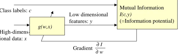
ci} as samples of a continuous-valued random variable X , xi ∈RD, and class labels as samples of a discrete-valued random variable C, ci∈ {1,2,...,Nc},i∈ {1,...,N}, the objective is to find a transformation g (or its parameter vector w) to yi∈Rd,d <D, such that yi =g(w,xi)maximizes
I(C,Y), the mutual information (MI) between transformed data Y and class labels C. The procedure is depicted in Figure 1. To achieve this, I(C,Y)needs to be estimated as a function of the data set, I({ci,yi}), in a differentiable form. Once that is done, gradient ascent can be performed on I(C,Y) as follows (denoting the learning rate byη)
wt+1=wt+η
∂I
∂w=wt+η N
∑
i=1
∂I
∂yi
∂yi
∂w . (4)
Following sections outline how to calculate this non-parametric estimate I({ci,yi}).
Class labels: c
High-dimens-ional data: x
g(w,x)
Mutual Information I(c,y)
(=Information potential)
Gradient Low dimensional features: y
w I
∂ ∂
Figure 1: Learning feature transforms by maximizing the mutual information between class labels and transformed features.
3. Renyi Entropy Reduces to Pairwise Interactions
We recapitulate the results of Principe et al. (2000) in using Renyi entropy combined with Parzen window density estimation. We emphasize that we will not be using Renyi entropy directly. The
purpose of this section is to show how measures involving quadratic forms of densities can be easily estimated directly from samples in a non-parametric fashion. This serves also as a motivation to find a similar measure for mutual information.
3.1 Renyi Entropy
Shannon derived the entropy measure H (Equation 1) from his three axioms that such a measure should fulfill (Shannon, 1948). However, Kapur (1994) argues that when the aim is not to compute an accurate value of the entropy of a particular distribution, but rather to find a distribution that maximizes or minimizes the entropy given some constraints, then Shannon’s third axiom of additiv-ity/recursivity is not necessary. This leads to a large number of alternative entropy measures, each of which produces the same distribution as the result of optimization. The choice of an appropri-ate measure can then be made, for example, by the convenience of use (Kapur, 1994, Kapur and Kesavan, 1992).
One such entropy measure is Renyi entropy (Renyi, 1961, Kapur, 1994). In fact, this is a para-metric family of measures which includes Shannon entropy as one particular case. For a discrete variable C, and for a continuous variable Y , Renyi entropy of orderαis defined as
HRα(C) = 1
1−αlog
∑
c p(c)α; H
Rα(Y) = 1 1−αlog
y
p(y)αdy , (5)
whereα>0,α=1, and limα→1HRα=H. We will be concerned with quadratic measures (α=2) for reasons that become clear in the following subsection.
3.2 Parzen Density Estimation
Entropy measures of continuous variables are based on probability density functions of the variables. One non-parametric method to estimate the densities is the Parzen window method (Parzen, 1962). The method involves placing a kernel function on top of each sample and evaluating the density as a sum of the kernels. It turns out that Renyi’s quadratic measure, when combined with Parzen density estimation method using Gaussian kernels, provides significant computational savings.
The Gaussian kernel in d-dimensional space is defined as
G(y,Σ) = 1
(2π)d2|Σ|12
exp
−1 2y
TΣ−1y
.
Now, for two kernels, the following holds
y
G(y−ai,Σ1)G(y−aj,Σ2)dy=G(ai−aj,Σ1+Σ2). (6) Thus, the convolution of two Gaussians centered at ai and aj is a Gaussian centered at ai−aj with covariance equal to the sum of the original covariances. This property facilitates evaluating Renyi’s quadratic entropy measure, which is a function of the square of the density function. Assume now that the density of Y is estimated as a sum of spherical Gaussians each centered at a sample yi (Parzen density estimator),
p(y) = 1
N
N
∑
i=1
The symbol I denotes a unit matrix. Then it follows that the quadratic Renyi entropy in (5) equals
HR2(Y) = −log
y
p(y)2dy
= −log 1
N2
y
N
∑
k=1 N
∑
j=1
G(y−yk,σI)G(y−yj,σI)
dy
= −log 1
N2 N
∑
k=1 N
∑
j=1
G(yk−yj,2σI). (8)
Thus, Renyi quadratic entropy can be estimated as a sum of local interactions, as defined by the kernel, over all pairs of samples. Because of symmetry, only half of these need to be evaluated in practice.
4. Quadratic Mutual Information
This section develops expressions for “quadratic mutual information” based on non-parametric mea-sures similar to Renyi quadratic entropy.
4.1 Quadratic Divergence Measures
As seen, the entropy of a multivariate density function is readily computable in a non-parametric fashion from a sample data set as interactions between pairs of samples. This concept needs to be extended now to mutual information between variables. To apply (6), mutual information should either be expressed as a function of the densities of the variables squared, or in some other form that can be expressed as convolutions of kernel functions.
As discussed in Section 2.1, MI can be viewed as KL divergence between the joint density and the product of the marginal densities of the variables. We view now alternative divergence measures for this purpose.
Kapur (1994) argues that if the aim is not to calculate an absolute value of the divergence, but rather to find a distribution that minimizes/maximizes the divergence, the axioms used in deriving the measure can be relaxed and yet the result of the optimization is the same distribution (Kapur, 1994, p. 178). Kapur (1994) presents a large number of such measures for two discrete distributions P and Q, one of which is the following (Kapur, 1994, p. 178)
D(P,Q) = 1
α(α−1) n
∑
i=1
piα−αpiqiα−1+ (α−1)qαi
, α=0,α=1. (9)
Selectingα=2, ignoring a constant, and extending the measure in (9) to continuous densities gives simply
D(f,g) =
x(
f(x)−g(x))2dx, (10) which is also suggested in Kapur and Kesavan (1992, p. 153). It is clear that the measure is always positive, and when f(x) =g(x)for all x, it evaluates to zero.
(see Topsøe, 2000, and references therein), several further divergence measures can be written, one of which is the variational distance
V(f,g) =
x|
f(x)−g(x)|dx.
Pinsker’s inequality gives a lower bound on K(f,g)≥12V(f,g)2 (Topsøe, 2000). Since f(x)and g(x)are probability density functions, both are between zero and one, and|f(x)−g(x)| ≥(f(x)−
g(x))2, resulting in V(f,g)≥D(f,g). Thus, maximizing D(f,g) is equivalent to maximizing a lower bound to K(f,g).
Since mutual information is expressed as the divergence between the joint density and the prod-uct of the marginals, we can insert them into (10), leading to a quadratic mutual information measure between two continuous variables Y1and Y2(denoted by IT henceforth):
IT(Y1,Y2) =
(p(y1,y2)−p(y1)p(y2))2dy1dy2 . (11)
4.2 Quadratic Mutual Information in the Discrete Case
It is now straightforward to extend the quadratic mutual information expression to discrete variables (class labels).
Assume that we have data as samples of a continuous valued random variable X in RD, and for each sample xi we have a corresponding class label ci∈ {1,2,...,Nc}. We write now expressions for quadratic mutual information between the transformed data y=g(w; x)and corresponding class labels c. The purpose is to find such a transform, or such parameters w for the transform, that results in maximum MI between Y and C. At this stage, no assumptions about the transform g need to be made.
With continuous-valued Y and discrete C, the quadratic mutual information is as follows:
IT(C,Y) =
∑
c
y
p(c,y)2dy+
∑
c
y
P(c)2p(y)2dy−2
∑
c
y
p(c,y)P(c)p(y)dy . (12)
Let us make the following definitions of the quantities appearing in (12):
VIN ≡
∑
c
y
p(c,y)2dy VALL ≡
∑
c
y
P(c)2p(y)2dy VBTW ≡
∑
c
y
p(c,y)P(c)p(y)dy . (13)
With these,
IT(C,Y) =VIN+VALL−2VBTW . (14)
The gradient of I per sample∂∂yI
i that is needed in (4) will be
∂IT
∂yi =
∂VIN
∂yi +
∂VALL
∂yi −
2∂VBTW
∂yi .
4.3 Information Potentials
Now we develop expressions for the Parzen density estimates of p(y) and p(c,y), and we insert
those into (14).
Assume that we have Jpsamples for each class cp. Then, the class prior probabilities are P(cp) =
Jp/N, with∑Npc=1Jp=N.
We use two different notations for the samples of data Y in the output space. A sample is written with a single subscript yi when its class is irrelevant; index 1≤i≤N. If the class is relevant, we write yp j, with the class index 1≤p≤Nc, and the within-class index 1≤ j≤Jp.
The density of each class cp, as a Parzen estimate using a symmetric kernel with width σ, is written as
p(y|cp) = 1 Jp
Jp
∑
j=1
G(y−yp j,σ2I) . Since the joint density is written as p(c,y) =p(y|c)P(c), we have
p(cp,y) = 1 N
Jp
∑
j=1
G(y−yp j,σ2I), p=1,...,Nc . (16) The density of all data is p(y) =∑cp(c,y). Thus we have
p(y) = 1
N
Nc
∑
p=1 Jp
∑
j=1
G(y−yp j,σ2I) = 1 N
N
∑
i=1
G(y−yi,σ2I) . (17) Using a set of samples in the transformed space{yi}, we insert (16) and (17) into (13). Making use of (6) and (8), we get
VIN({ci,yi}) =
∑
c
y
p(c,y)2dy= 1 N2
Nc
∑
p=1 Jp
∑
k=1 Jp
∑
l=1
G(ypk−ypl,2σ2I) (18)
VALL({ci,yi}) =
∑
c
y
P(c)2p(y)2dy= 1 N2
Nc
∑
p=1
Jp
N
2 N
∑
k=1 N
∑
l=1
G(yk−yl,2σ2I) (19)
VBT W({ci,yi}) =
∑
c
y
p(c,y)P(c)p(y)dy= 1 N2
Nc
∑
p=1 Jp
N
Jp
∑
j=1 N
∑
k=1
G(yp j−yk,2σ2I) . (20) Despite the three summations above, these are only double sums over the samples (because of class-based indexing). These kinds of quantities can be called “information potentials” in analogy to physical particles (Principe et al., 2000). Given the fact that class information is now taken into account, there is an interesting interpretation of the pairwise interactions between samples, or “information particles”:
• VIN can be seen as interactions between pairs of samples inside each class, summed over all classes.
• VALLconsists of interactions between all pairs of samples, regardless of class, weighted by the sum of squared class priors.
4.4 Information Forces
Derivatives of these potentials with respect to samples represent “information forces”, i.e., directions and magnitudes where the “particles” would like to move (actually, to have the transform move them) in the output space in order to maximize the objective function. To this effect, the chain rule can then be simply applied to change the parameters w of the transform g.
First, we need the derivative of the potential (i.e., the force between two samples), which is given as
∂ ∂yi
G(yi−yj,2σ2I) =G(yi−yj,2σ2I)(
yj−yi) 2σ2 . With this, we get
∂ ∂yci
VIN= 1 N2σ2
Jc
∑
k=1
G(yck−yci,2σ2I)(yck−yci) . (21) This represents a sum of forces that other “particles” in class c exert to particle yci (direction is towards yci). For the derivative of VALL, we get
∂ ∂yci
VALL= 1 N2σ2
Nc
∑
p=1
Jp
N
2 N
∑
k=1
G(yk−yi,2σ2I)(yk−yi) . (22)
This represents a sum of forces that other “particles”, regardless of class, exert to particle yci. Note that this particle is also denoted as yiwhen the class c is irrelevant. Direction is again towards
yi. The derivative of VBTW is
∂ ∂yci
VBTW = 1 N2σ2
Nc
∑
p=1 Jp+Jc
2N Jp
∑
j=1
G(yp j−yci,2σ2I)(yp j−yci) . (23)
This component appears in negative form in (15). Its effect is away from yci, and it represents the repulsion of classes away from each other.
Inserting these derivatives into the gradients of IT (15) and into (4) results in a gradient ascent algorithm to maximize the MI.
5. Linear Feature Transforms
This section presents an example of the transform-dependent factor∂yi/∂w in (4).
5.1 Matrix Parametrization
To find a linear, dimension-reducing transform, we search for a subspace Rd, d<D, such that the mutual information between class labels, and the data projected onto this subspace, is maximized. Thus,
W=argmax
W (
I({ci,yi})); yi=WTxi , (24)
The simplest way to take the constraint into account is to update W using any appropriate unconstrained optimization technique, and then to project W back to the constraint set. In this case, the projection step is accomplished by orthonormalizing W after each update.
In addition to gradient ascent, any optimization methods that make use of the curvature of the objective function, such as Quasi-Newton or Conjugate Gradients, can be used here. Levenberg-Marquardt also works well, even though the objective function does not strictly fulfill the assump-tions.
Another possible parametrization of the transform matrix, as Givens rotations, has been outlined by Torkkola and Campbell (2000).
5.2 Visualization of Class Separation
We present visualization experiments with synthesized data, and with some publicly available datasets. In these examples we learn a linear projection from a high-dimensional feature space onto a plane for visualization purposes, especially to visualize class separability. For an actual pat-tern recognition application, a projection onto a higher dimensional space would be preferred (see Section 6.2).
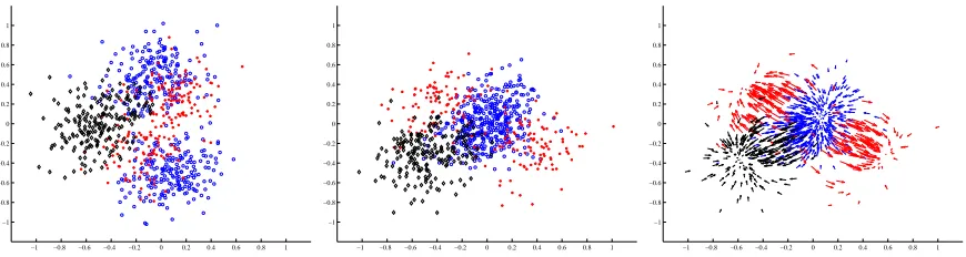
The first example is synthetic with non-Gaussian densities. It is designed to have a local opti-mum, in addition to a global one. The purpose of this example is to illustrate how LDA, assuming Gaussian classes, fails to find the global optimum. The dataset is three-dimensional, and has three classes. Class one has 400 samples from a bimodal Gaussian distribution (blue circles), with cen-ters at (1,0,0) and (-1,0,0). Class two has 200 samples (red asterisks), also drawn from a bimodal Gaussian distribution, with centers at (0,1,0) and (0,-1,0).
Optimal projection would, of course, face the configuration. To disturb, we added a third class, 200 samples of a single Gaussian at (0,0.7,1), in front of the configuration (black diamonds). Since we have three classes, LDA is able to produce a two-dimensional projection, which is depicted in the left side of Figure 2. This projection views the data along the class two axis, and it is a local maximum of the MI. A classifier based on this projection would have difficulties separating class two (red asterisks) from the other classes.
LDA was used as the initial state to learn the MMI-projection. The result is presented in the middle part of Figure 2. In about five iterations of Levenberg-Marquardt optimization, with a
rela-−1 −0.8 −0.6 −0.4 −0.2 0 0.2 0.4 0.6 0.8 1 −1
−0.8 −0.6 −0.4 −0.2 0 0.2 0.4 0.6 0.8 1
−1 −0.8 −0.6 −0.4 −0.2 0 0.2 0.4 0.6 0.8 1 −1
−0.8 −0.6 −0.4 −0.2 0 0.2 0.4 0.6 0.8 1
−1 −0.8 −0.6 −0.4 −0.2 0 0.2 0.4 0.6 0.8 1 −1
−0.8 −0.6 −0.4 −0.2 0 0.2 0.4 0.6 0.8 1
tively wide Parzen kernel, the method converged to the global optimum, which now exhibits much better separation for the second class (red asterisks). The actual mutual information, using (14), increased from 1.02.10−4to 1.28.10−4.
In this example, as well as in general, it is useful to have a kernel width that approximately gives each sample an influence over every other sample. A simple rule that seems to work well is to take the distance of the two farthest points in the output space, and use a kernel width σof about half of that. Figure 2 depicts the information forces in the final state, that is, the directions where each sample would move in the output space were it free to do so. These forces are propagated back to the transform, and the parameters of the transform are changed such that the samples will move in the desired directions in the output space.
The forces become more local as the kernel width is narrowed down. This suggests a determin-istic annealing procedure where one would begin with a wide kernel and narrow it down towards the end of the optimization (Rose et al., 1990). A wide kernel forces larger clusters of data in different classes to separate first. As the width shrinks, the adaptation will focus on the finer details of the class distributions. This kind of a procedure serves two purposes, first, helping to escape from the local maxima induced by the data, and second, fine-tuning the parameters of the transform, if the transform has enough degrees of freedom. This procedure helped to escape from the local optimum of the initial LDA projection. A working (but heuristic) choice for the final kernel width could be half of the average within-class distance in the output space.
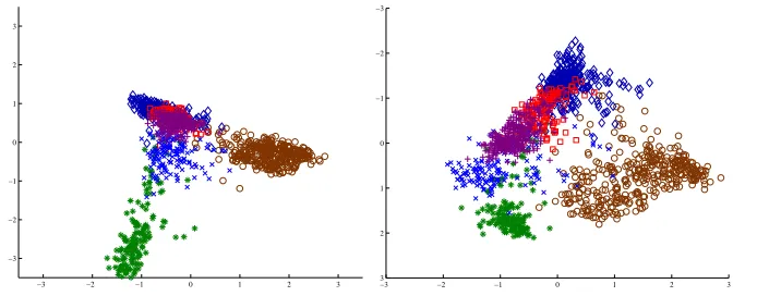
A second example illustrates a projection from 36-dimensional feature space onto two. This is the Landsat satellite image database from UCI Machine Learning Repository. The data has six classes. LDA- and MMI-projections are depicted in Figure 3. LDA separates two of the classes very well but places the other four almost on top of each other. The criterion of LDA is a combination of both intra-class compactness and inter-class separation. This has been achieved: all classes are represented as quite compact clusters — unfortunately they are on top of each other. Two of the classes and a third cluster comprising of the four remaining classes are well separated.
MMI has produced a projection that attempts to separate all classes. The four classes that LDA was not able to separate appear to lie on a single continuum and blend into each other. MMI, not being constrained by the assumption of making the class densities look Gaussian, has found a projection orthogonal to that continuum while still keeping the other two classes well separated, but not necessarily as compact.
−3 −2 −1 0 1 2 3
−3 −2 −1 0 1 2 3
−3
−2
−1
0
1
2
3
−3 −2 −1 0 1 2 3
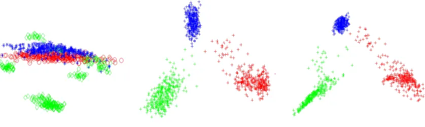
Finally, Figure 4 illustrates the differences and similarities between PCA, LDA and MMI pro-jections. PCA obviously pays no attention to class separation, LDA attempts to represent the classes as compact Gaussian clusters, while MMI has no such restrictions. Note also that if the kernel width is kept large, MMI produces a projection that is almost exactly the LDA projection. This has the ef-fect of smearing out any finer details in class densities and makes the adaptation algorithm perceive each class as a single Gaussian with a large variance.
Figure 4: Three classes in 12 dimensions projected onto a two-dimensional subspace using PCA (left), LDA or MMI with a wide kernel (middle), and MMI using a narrow kernel (right). This is the “Pipeline flow” database.
6. Learning Nonlinear Feature Transforms
While linear transforms are certainly useful in visualization and in pattern recognition applications (see Section 6.2), there are cases where nonlinear feature transforms might be more appropriate. We now discuss implementations of such transforms using a particular type of universal approximator network, Radial Basis Function (RBF) network. Bishop (1995) gives a nice overview of these networks. Another type of universal approximator network, Multilayer Perceptron, can also be used in this context (Torkkola, 2001b). The only difference in learning linear transforms will now be the latter factor in (4),∂yi/∂w.
6.1 Radial Basis Function Networks
For an RBF, the task of computing∂yi/∂w, the derivative of the output with respect to the parameters of the network, is the standard gradient calculation. Since this is presented in many textbooks, for example, by Bishop (1995), we do not repeat it here.
Data set Dim. Classes Training set size Test set size
Letter 16 26 16000 4000
Landsat 36 6 4435 2000
Phoneme 20 20 1962 1961
Pipeline Flow 12 3 1000 1000
Pima 8 2 500 200
Table 1: Characteristics of the data sets used in classification experiments.
A normal design procedure for RBF networks is unsupervised training of the basis functions using EM followed by supervised training of the linear output weights (Bishop, 1995). We exper-imented by training only the linear part using the MMI criterion, keeping the basis functions fixed after the EM algorithm. This resulted in no loss or minimal loss of accuracy compared to full su-pervised training of all network parameters using MMI. Since the computation involved in the latter is not insignificant, all classification experiments reported in this paper involving RBF networks are performed with the former configuration.
Furthermore, direct connections from the input to the output were added, which improved per-formance. This is also included in all reported experiments. An illustration of an RBF network learning to transform three-dimensional features into two is available.6
6.2 Classification Experiments with Linear and Non-Linear Transforms and Feature Selection
Classification experiments were performed using five data sets that are very different in terms of dimensionality, number of classes, and the amount of data. The sets and some of their characteristics are presented in Table 1. The Phoneme set is available with the LVQ PAK,7and the Pipeline Flow set is available from the Aston University.8 The rest of the data sets are from the UCI Machine Learning Repository.
Two classifiers were used. The first one is Learning Vector Quantization (LVQ) as implemented in package LVQ PAK (Kohonen et al., 1992). An important parameter of this classifier is the num-ber of code vectors, which determine the decision borders between classes. These were chosen approximately according to the number of training examples for each database: Letter — 500, Landsat and Phoneme — 200, Pipeline Flow — 25, and Pima — 15 code vectors. Each error figure presented is an average of ten LVQ classifiers trained with different random example presentation orders.
A Support Vector Machine (SVM) implementation, called SVMTorch, was used as a second classifier (Collobert and Bengio, 2001). A Gaussian kernel was used in all experiments. For both classifiers, the evaluation procedure consists of learning the dimension-reducing transform from the training set, applying the transform to both training and test sets, training a classifier using the transformed training set, and finally, evaluating the classifier using the transformed test set. Results comparing the linear transforms (PCA, LDA and MMI) to a nonlinear transform (RBF trained using MMI criterion) are presented in Tables 2 – 6 in terms of classification error rates on the test sets.
6. See http://members.cox.net/torkkola/mmi.html and compare the 2nd video clip (linear transform, 3d→2d) to an RBF-transform starting from random parameters (5th video clip).
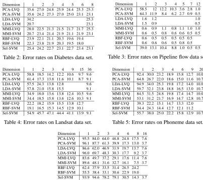
Dimension 1 2 3 4 5 6 8 PCA-LVQ 35.6 27.0 24.8 25.9 24.4 25.3 25.3 PCA-SVM 35.6 24.2 27.3 27.0 25.0 23.1 23.1
LDA-LVQ 34.2 25.3
LDA-SVM 20.7 23.1
MMI-LVQ 28.0 22.5 21.3 21.5 21.7 21.7 25.3 MMI-SVM 20.7 23.4 21.4 21.9 21.1 21.9 23.1 RBF-LVQ 23.9 22.1 21.1 20.3 19.6 19.4 RBF-SVM 22.3 23.8 21.9 20.3 19.5 18.0 Sel-SVM 25.4 24.2 22.7 23.1 22.7 23.4 23.1
Table 2: Error rates on Diabetes data set.
Dimension 1 2 3 4 5 7 12
PCA-LVQ 58.5 12 12.2 10.3 3.6 2.8 1.0 PCA-SVM 64.3 11.9 8.4 6.2 2.7 0.9 0.5
LDA-LVQ 1.6 1.2 1.0
LDA-SVM 1.5 0.9 0.5
MMI-LVQ 0.6 0.9 1.1 0.8 1.1 1.0 1.0 MMI-SVM 0.6 0.5 0.8 0.6 0.6 0.5 0.5 RBF-LVQ 0.6 0.5 0.5 0.5 0.5 0.5 RBF-SVM 0.6 0.6 0.6 0.5 0.8 0.5 Sel-SVM 39.0 13.1 10.4 8.8 1.0 0.5 0.5 Table 3: Error rates on Pipeline flow data set.
Dimension 1 2 3 4 9 15 36
PCA-LVQ 58.8 18.5 14.2 12.2 10.6 9.7 9.6 PCA-SVM 61.4 17.3 13.8 11.6 10.1 8.7 9.1 LDA-LVQ 57.5 24.3 13.8 12.8 9.6 LDA-SVM 57.8 21.0 15.8 15.5 9.1 MMI-LVQ 34.9 18.0 13.6 13.8 12.4 10.5 9.6 MMI-SVM 34.4 18.5 15.8 13.6 12.6 10.3 9.1 RBF-LVQ 22.2 18.2 15.9 15.5 13.8 12.7 RBF-SVM 19.1 16.5 15.3 14.5 12.9 10.1 Sel-SVM 54.9 45.7 47.1 44.4 41.1 13.9 9.1
Table 4: Error rates on Landsat data set.
Dimension 1 2 3 4 6 9 20
PCA-LVQ 92.4 30.0 23.2 18.9 15.8 12.7 10.0 PCA-SVM 64.8 26.7 22.0 18.6 15.0 11.6 10.7 LDA-LVQ 94.9 34.0 25.3 19.8 17.2 14.0 10.0 LDA-SVM 59.7 32.1 23.8 18.8 16.5 13.0 10.7 MMI-LVQ 84.5 31.5 24.8 19.8 17.4 14.7 10.0 MMI-SVM 53.1 31.2 21.7 16.9 14.7 12.8 10.7 RBF-LVQ 39.3 22.2 15.1 14.7 13.3 12.0 RBF-SVM 34.4 24.3 14.4 12.7 12.1 11.2 Sel-SVM 55.7 38.0 25.0 22.2 15.8 12.9 10.7 Table 5: Error rates on Phoneme data set.
Dimension 1 2 3 4 6 8 16
PCA-LVQ 95.5 84.0 64.0 46.8 24.8 17.5 7.6 PCA-SVM 96.1 87.7 61.3 39.9 17.3 13.0 3.7 LDA-LVQ 86.6 62.0 46.9 31.9 19.7 13.7 7.6 LDA-SVM 96.0 69.7 48.3 30.3 17.7 9.2 3.7 MMI-LVQ 83.6 49.7 37.2 29.1 17.6 11.4 7.6 MMI-SVM 89.6 48.1 31.6 32.7 16.1 7.5 3.7 RBF-LVQ 62.4 37.9 33.5 31.4 26.5 24.2 RBF-SVM 55.5 38.4 33.1 30.6 22.9 19.0 Sel-SVM 93.9 94.6 78.2 79.1 30.5 14.3 3.7
Table 6: Error rates on Letter data set.
MMI transforms were initialized by LDA and by five different random parameter choices. After optimization, the transform with the largest MI was chosen as the result. However, using a shrinking kernel, with the choices mentioned in Section 5.2, had the effect of all initializations converging to the same solution in all but a few cases.
The diversity of the data sets is reflected in the relation between error rates obtained using PCA and LDA. LDA is better when the data fits the assumptions of LDA (Letter, Pipeline, Pima). PCA turned out to outperform LDA in many projections with Landsat and Phoneme sets. We hypothesized that major classes in these two data sets lie at the “edges” or “corners” of the feature space. Though PCA is only concerned with finding maximum directions of the total data covariance, it is actually finding directions that separate class means in these cases. We tested the hypothesis by using the class mean covariance Sbas the criterion (this is the latter part of the LDA criterion). The resulting projections were almost exactly the same as those that PCA produces, confirming the hypothesis.
Nonlinear transforms appear to be particularly useful in transformations to low dimensions, especially in cases where the class borders have complex structures (Letter, Phoneme). In view of these results, RBF networks appear to offer excellent capabilities as feature transforms to low dimensions, and in some cases, even to higher dimensions (Phoneme and Pima data sets). Results using MLP networks were inferior to RBF networks, and they are not included.
In general, the two classifiers behave in very similar fashion. SVM appears to outperform LVQ in more complex tasks with a large number of classes.
In addition to transforms, feature selection results are presented using the SVM classifier. Orig-inal features were ranked using MMI between a single feature and the class labels as the criterion according to (12). A number of best-ranked features were then selected.
Greedy selection is clearly inferior to transforms in cases such as the Landsat data set, where many correlated features are present (such as pixels of images), and thus, relevant information is distributed among many features. The error rate hardly decreases at all between selection of 2-9 features. This is evidently due to the same hidden variable, appearing as multiple features, being repeatedly selected.
The phoneme data set represents a different end of the spectrum regarding feature selection. Features in this set consist of cepstral coefficients that are nearly uncorrelated with each other. Error rates using selection are thus nearly as low as error rates of linear transforms (although nonlinear transforms do much better). For greedy feature selection, it pays to de-correlate the features before selection (or perhaps to apply ICA) to avoid this problem. Section 8 further discusses this case.
A problem plaguing nonlinear transforms appears to be the relative degradation of performance as the dimension of the output (transformed) space increases. This could be attributable to one of two reasons. First, Parzen density estimation does suffer from increasing dimensionality, especially when the number of samples remains constant. This is the familiar “curse of dimensionality”. There simply are not enough samples (regardless of the number) to reliably construct a kernel density estimate in higher dimensional spaces. A related issue is that the relative volume of the “sphere of influence” of a sample, as determined by the kernel width, decreases exponentially as the dimension increases. This fact complicates the selection of an appropriate kernel width for a given output dimension.
Second, generalization may be an issue with flexible nonlinear transforms when coupled with small amounts of training data. A remedy would be enforcing “stiffer” transforms via regularization, for example, by using weight decay.
7. Reducing Computation
In essence, we are trying to learn a transform that minimizes the class density overlap in the out-put space while trying to drive each class into a singularity. Since kernel density estimate results in a sum of kernels over samples, any kind of a divergence measure between two densities necessarily requires O(N2)operations. The only alternatives to reduce this complexity are either to reduce N, or to form simpler density estimates.
A straightforward way to achieve the former is random sampling. We discuss this approach, and we present the resulting practical algorithm in pseudocode form in Appendix A.
The latter alternative can be accomplished by means of a semi-parametric density estimator, such as a Gaussian Mixture Model (GMM). A GMM is learned in the low-dimensional output space for each class. Instead of evaluating interactions between samples, evaluating interactions between mixture components suffices. This approach also requires a GMM in the high-dimensional input space in order to realize learning of the transform between the two spaces. Appendix B discusses how this can be done without having to operate in the high-dimensional input space.
8. Some Limitations of Feature Transform and Feature Selection Methods
This section attempts to answer the following questions. Does a high dimensionality of the original feature space pose difficulties to the proposed method? Under what circumstances would selection methods be preferable to transform methods, and vice versa? We explore the issues experimentally by artificial data sets, in which several parameters are varied:
1. the number of classes Nc(3, 10, 30),
2. the amount of training data N (200, 1000, 5000 samples),
3. the way information is hidden in noise (concatenation of noise, or embedding in noise), 4. the dimension of the noise feature space D (0, 100, 1000, 10000).
A further purpose is also to demonstrate that, in a computational sense, none of these variables is a limitation to the methodology discussed in this paper.
In this experiment, the information-bearing data is intrinsically two dimensional, consisting of spherical Gaussian clusters equispaced on a unit circle, with each cluster representing a different class. All classes have the same variance, 0.3 times the distance between clusters. The test set had 5000 samples in every case.
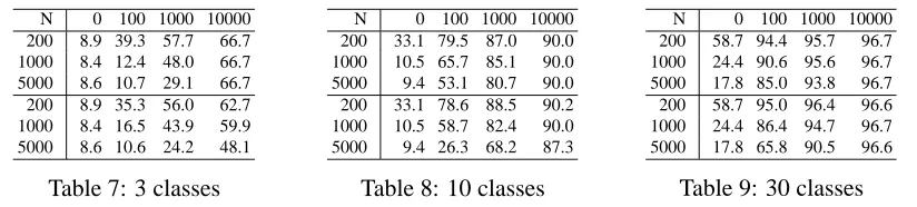
8.1 Concatenating Noise to Data
In the first experiment, D extra features consisting of independent Gaussian noise are concatenated to the feature set. The task for feature selection is to pick the two best features. As in Section 6.2, mutual information between the labels and the feature according to (12) was used as the criterion. Likewise, for feature transforms, the task was to find the best linear transform from the 2+D di-mensional space onto a two-didi-mensional space using the same criterion. The GMM-MMI approach of Appendix B was used in learning the transform. Results are presented in Tables 7 - 9 using SVM as the classifier.
This task is, in fact, an ideal case for feature selection, which did not fail once in picking the correct two features. Error rates using selection are thus equal to those with no noise concatenated (under column “0”). Thus, the tables only present feature transform results.
N 0 100 1000 10000 200 8.9 39.3 57.7 66.7 1000 8.4 12.4 48.0 66.7 5000 8.6 10.7 29.1 66.7 200 8.9 35.3 56.0 62.7 1000 8.4 16.5 43.9 59.9 5000 8.6 10.6 24.2 48.1
Table 7: 3 classes
N 0 100 1000 10000 200 33.1 79.5 87.0 90.0 1000 10.5 65.7 85.1 90.0 5000 9.4 53.1 80.7 90.0 200 33.1 78.6 88.5 90.2 1000 10.5 58.7 82.4 90.0 5000 9.4 26.3 68.2 87.3
Table 8: 10 classes
N 0 100 1000 10000 200 58.7 94.4 95.7 96.7 1000 24.4 90.6 95.6 96.7 5000 17.8 85.0 93.8 96.7 200 58.7 95.0 96.4 96.6 1000 24.4 86.4 94.7 96.7 5000 17.8 65.8 90.5 96.6
Table 9: 30 classes Tables 7 - 9: Noise features concatenated to data. Top halves: error rates with data and noise in high dimensions, bottom halves: data and noise transformed down to two features. Each row represents a different number of training samples, each column a different number of noise features concatenated to data.
using SVMs in the resulting two-dimensional space. In many cases the transform is able to improve the error rate substantially. However, this experiment underlines one inherent problem with feature transform methods that selection methods avoid. When the number of features that are irrelevant, is orders of magnitude larger than the number of useful features, transform methods produce a combination of many noise components as a result (together with the information). Being able to estimate the transform with enough statistical accuracy to ignore all irrelevant features requires more training items than provided in this experiment. However, sparse data may be different in this respect.
Each of the columns approaches the Bayes error rate as the number of training samples in-creases. It is evident that learning and applying the transform before training the classifier makes more efficient use of the data than training the classifier directly with all features. This can be seen in faster decrease of the error rate, in the lower half of the tables, as training sample size increases.
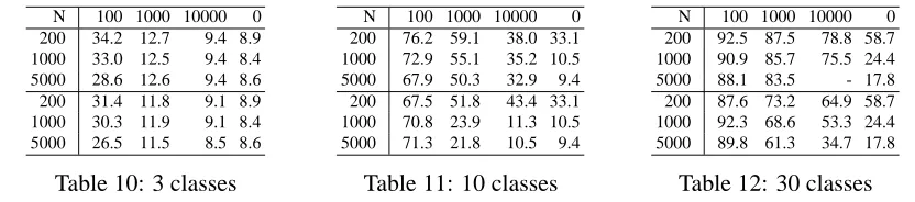
8.2 Embedding Data in Noise
The second experiment embeds data into a high dimensional space by generating a random D×2 matrix E, in which each individual element is drawn from a zero-mean Gaussian distribution with variance of one. Embedded data XE =EX+N, where X is the original data matrix, and each element of N is normally distributed with seven times the variance of EX. Each of the 100, 1000, or 10000 generated features now carries a little bit of information about the original features, hidden under additive noise. This represents the worst possible case for feature selection. Indeed, in every experiment, feature selection produced error rates close to random guessing. Tables 10 - 12 display the results with feature transforms to two-dimensions only.
In this case, the more available features, the more information there is about the discrimination task. This is reflected by the decrease in error rates as the dimensionality of the embedding data increases. Column “0” displays error rates using the original two-dimensional data.
Any transform can only retain or decrease the information contained in the original features. Thus, in principle, error rates should increase after the transform (moving from top halves to bottom halves). However, since there are sometimes large drops in the error rate, it appears to be useful to make the relevant information explicit to the classifier.
N 100 1000 10000 0 200 34.2 12.7 9.4 8.9 1000 33.0 12.5 9.4 8.4 5000 28.6 12.6 9.4 8.6 200 31.4 11.8 9.1 8.9 1000 30.3 11.9 9.1 8.4 5000 26.5 11.5 8.5 8.6
Table 10: 3 classes
N 100 1000 10000 0 200 76.2 59.1 38.0 33.1 1000 72.9 55.1 35.2 10.5 5000 67.9 50.3 32.9 9.4 200 67.5 51.8 43.4 33.1 1000 70.8 23.9 11.3 10.5 5000 71.3 21.8 10.5 9.4
Table 11: 10 classes
N 100 1000 10000 0 200 92.5 87.5 78.8 58.7 1000 90.9 85.7 75.5 24.4 5000 88.1 83.5 - 17.8 200 87.6 73.2 64.9 58.7 1000 92.3 68.6 53.3 24.4 5000 89.8 61.3 34.7 17.8
Table 12: 30 classes Tables 10 - 12: Data embedded in a high dimensional space with additive noise. Top halves: error rates with high-dimensional data, bottom halves: data + noise transformed down to two features. Each row represents a different number of training samples, each column a different dimension of the embedded feature space.
cases may fall between the two extremes presented in Sections 8.1 and 8.2, as demonstrated in results with the Landsat and Phoneme data sets in Section 6.2. Thus, a good strategy might be first to discard a number of irrelevant features followed by a transformation of the remaining features.
Another point clearly demonstrated by experiments in this section is the sheer impracticality of training support vector machines with large amounts of dense high-dimensional data. The 30 class case with 10000 features and 5000 training samples tended to produce a support vector set of size 12GB, and take 24 hours of 1GHz machine CPU time.9 On the other hand, learning the GMM-MMI feature transform from 10000 dimensions to two took only 2 minutes in the same case, followed by SVM training of about the same duration, with the result of even decreasing the error rate.
9. Previous Work
Linear feature transforms based on some kind of a class overlap measure have been discussed at length by Devijver and Kittler (1982). Most of these measures, including the Shannon mutual information, are nearly impossible to evaluate in the general multi-class case without resorting to modeling classes as single Gaussians. Even then, there is no analytical solution (unless all class covariances are assumed equal) — one has to resort to numerical optimization. Some examples of successful applications of such measures have been presented, for example, by Guorong et al. (1996) and Saon and Padmanabhan (2001).
However, there is one exception that allows for non-parametric density estimates — a measure introduced by Patrick and Fisher II (1969) for class separability:
JD=
y[
p(y|c1)P(c1)−p(y|c2)P(c2)]2dy
1
2
.
This is, in fact, the same measure as (10). Previous work using this measure (Patrick and Fisher II, 1969, Hillion et al., 1988, Aladjem, 1998) has concentrated on feature selection, binary classification case, and on finding a single discriminant direction. In contrast, we are simultaneously computing a number of features that jointly maximize the MI-measure, and in a way that is usable with large data sets.
Principe et al. (2000) started from the Renyi entropy estimate, and heuristically derived mea-sures for MI having quadratic forms similar to Renyi entropy. First, they considered some known
inequalities for L2 distance measure between vectors in RD, and they then wrote analogous expres-sions for the divergence between two densities. Using the Cauchy-Schwartz inequality
xy ≥xTy⇔logx 2y2 (xTy)2 ≥0 , they write
KC(f,g) =log
f(x)2dxg(x)2dx ( f(x)g(x)dx)2 . The difference of vectors inequality
(x−y)T(x−y)≥0⇔ x2+y2−2xTy≥0 gives the expression
KT(f,g) =
f(x)2dx+
g(x)2dx−2
f(x)g(x)dx .
Both measures are always positive, and when f(x) =g(x)both measures evaluate to zero. However, KC is not a convex function while KT is, which is a desirable property of a divergence function (Kapur, 1994).
The measure KT is essentially the same divergence measure we use in this paper (Equation 10). However, in this work we formulate the problem between discrete and continuous variables, and we use the measure specifically to learn feature transforms. Principe et al. (2000) used the measure to maximize the MI between two continuous variables.
The Renyi entropy difference,
∆0HRα(Y1,Y2) = HRα(Y1,Y2)−HRα(Y1)−HRα(Y2)
= 1
1−αlog
p(y1,y2)αdy1dy2
p(y1)αdy1
p(y2)αdy2
,
bears some resemblance to KC. This measure is briefly mentioned in the context of image registra-tion by Hero et al. (2001). The measure has a further property of converging to the Shannon mutual information asα→1, by the merit of each individual component of the sum converging to their Shannon equivalents. Using α=2 would allow the same non-parametric treatment as Equation (11). Differences between these measures for the purposes of learning feature transforms have not been explored yet.
10. Conclusion
We have presented a method for feature extraction using as criterion an approximation of the mutual information between features and class labels. This approximation is inspired by the quadratic Renyi entropy. It is differentiable, and it can be numerically optimized to learn parameters of an arbitrary smooth feature transform. The two main advantages of the method are that:
2. Computationally, the method is usable with training datasets of the order of thousands or tens of thousands of samples. We also discussed two methods that extend this to larger databases, one based on a stochastic gradient approximation, the other on replacing the non-parametric Parzen density estimation by a semi-parametric method using Gaussian mixture models.
In static pattern recognition tasks, such feature transforms are clearly useful, as they appear to be able to extract more discriminatory information from the source features than, for example, the Fisher discriminants (LDA), as shown by experiments.
Judging from the experiments, the method appears to work extremely well only in transforms to low dimensions (10). Our conjecture is that the Parzen density estimation sets an upper limit to a usable output dimension. To at least partly overcome the limitation of the curse of the dimension-ality, it is possible to use the suggested method first to find a low-dimensional (2-8) discriminative subspace, then project the data into the space orthogonal to that subspace, and repeat the process until a desired number of features has been obtained.
Further work would include both theoretical and experimental evaluation of different divergence measures for mutual information maximization and minimization.
The method is also readily applicable to regression problems, by replacing the discrete class label by a continuous variable. In fact, this was the original formulation of Principe et al. (2000).
Appendix A: Reducing Computation by Random Sampling
Rather than computing the full gradient, as in the previous formulation, it is straightforward to devise a stochastic gradient algorithm.
The principle is as follows. Take a random sample of two transformed data points y1 and y2. These two points serve as a sample of the whole database. Using the Parzen estimate, compute the information potential and the information force between those two samples only. Make a small ad-justment to the parameters of the transform in the direction of the gradient. Details of the derivation have been presented by Torkkola (2002).
This two-sample stochastic gradient and the full gradient involving all interactions between all samples are really two ends of a single spectrum. In practice, if the full gradient is out of reach for computational reasons, it is more desirable to take as large a random number of sample pairs as computationally possible. This gradient should be now much closer to the true gradient rather than a gradient computed from just a small number of pairwise interactions. The sums in IT(C,Y) in Equations (14,18,19, 20) and in the gradient equations (15,21,23,22) now become single sums over the drawn sample pair set.
We summarize the resulting algorithm in Table 13. This represents the final practical form of the method based on Parzen density estimation. Another practical form is discussed in Appendix B. For example, for a data set consisting of 1000 samples, the full gradient evaluation consists of 106interactions to be evaluated for each iteration of the optimization. Instead, evaluating just 1000 randomly chosen pairwise interactions each iteration results in almost exactly the same convergence behavior, i.e., the gradient directions at each step are very close to the full gradient directions. Evaluating a mere 30 random interactions at each iteration results in somewhat more stochastic-looking convergence10, though the final solution is the same for each case. For any of the data sets
Initialize W0randomly (or by LDA) Y=W0X
σ=σ0(Y)(for example, maximum distance between samples / 2) repeat
repeat
draw M sample pairs{yi1,yi2}i,i=1,...,M,from Y at random (or use all of Y) Di=yi1−yi2, for all i
Gi=Gaussian(Di,σ), for all i
I=sum of Giaccording to (14,18,19,20) but using single sums
∂I/∂Wk=sum of GiDiaccording to (15,21,23,22) but using single sums Wk+1=orthonormalize(Wk+η∂I/∂Wk)
k=k+1
Y=WkX until I does not increase decreaseσ
untilσ<σf(Y)(for example, average distance within classes / 2) Table 13: Algorithm pseudocode.
used in classification experiments, the run time of a MATLAB-implementation is less than a minute when 4000 sample pairs are used in each iteration.
Appendix B: Reducing Computation by Gaussian Mixture Model Mappings
The second method for reducing the computation is to construct simpler class density estimates. In terms of complexity and flexibility, semi-parametric density estimates lie between the fully non-parametric Parzen estimator and a fully non-parametric estimate, such as a Gaussian.
Using Gaussian Mixture Models (GMM) as such a semi-parametric method retains two ad-vantages of the Parzen approach. First, GMMs are able to represent arbitrary class densities, and second, a GMM is a sum of Gaussians just as the Parzen density estimate is. Thus, Equations (6) and (8) can be applied to evaluate IT as a function of the mixture components instead of Parzen kernel functions. Quadratic Renyi entropy (8) and the terms in the quadratic mutual information measures IT (18—20) reduce to evaluating the interactions between mixture components.
For optimization in (4), we need to represent IT as a function of W as follows. A GMM for training data can be constructed in the low-dimensional output space. Note that to transform the data into the output space at this point, a random or an informed guess needs to be used as the transform.
The same samples are used to construct a GMM in the high dimensional input space using the same exact assignments, or weights of samples to mixture components as the output space GMMs. Running the EM-algorithm in the input space is now unnecessary since we know which samples belong to which mixture components. A similar strategy has been used to learn GMMs in high dimensional spaces (Dasgupta, 2000).
output space GMM, which is a linear transform of the input space GMM by W. Thus we can easily evaluate∂IT/∂W.
A great advantage of this strategy is that once the GMMs have been created, the actual training data needs not be accessed at all during optimization. A further advantage is the elimination of the need to operate in the high-dimensional input space, not even for estimating GMMs in the beginning of the procedure. Derivation of the adaptation algorithm and experiments have been presented by Torkkola (2001a). Illustrative video clips are placed on the web (see footnote 10).
References
M.E. Aladjem. Nonparametric discriminant analysis via recursive optimization of Patrick-Fisher distance. IEEE Transactions on SMC, 28(2):292–299, April 1998.
A. Antos, L. Devroye, and L. Gyorfi. Lower bounds for bayes error estimation. IEEE Transactions on PAMI, 21(7):643–645, July 1999.
R. Battiti. Using mutual information for selecting features in supervised neural net learning. Neural Networks, 5(4):537–550, July 1994.
C. M. Bishop. Neural Networks for Pattern Recognition. Oxford University Press, Oxford, New York, 1995. K.D. Bollacker and J. Ghosh. Linear feature extractors based on mutual information. In Proc. 13th ICPR,
pages 720–724, August 25-29 1996.
B.V. Bonnlander and A.S. Weigend. Selecting input variables using mutual information and nonparametric density estimation. In Proc. 1994 International Symposium on Artificial Neural Networks, pages 42–50, Tainan, Taiwan, 1994.
R. Collobert and S. Bengio. SVMTorch: Support Vector Machines for Large-Scale Regression Problems. Journal of Machine Learning Research, 1:143–160, 2001.
S. Dasgupta. Experiments with random projection. In Proc. 16th Conf. on Uncertainty in Artificial Intelli-gence, pages 143–151, Stanford, CA, June30 - July 3 2000.
P.A. Devijver and J. Kittler. Pattern recognition: A statistical approach. Prentice Hall, London, 1982. R.M. Fano. Transmission of Information: A Statistical theory of Communications. Wiley, New York, 1961. K. Fukunaga. Introduction to statistical pattern recognition (2nd edition). Academic Press, New York, 1990. M. Girolami, A. Cichocki, and S-I. Amari. A common neural network model for unsupervised exploratory data analysis and independent component analysis. IEEE Transactions on Neural Networks, 9(6):1495 – 1501, November 1998.
X. Guorong, C. Peiqi, and W. Minhui. Bhattacharyya distance feature selection. In Proc. 13th ICPR, vol-ume 2, pages 195 – 199. IEEE, 25-29 Aug. 1996.
M.E. Hellman and J. Raviv. Probability of error, equivocation and the chernoff bound. IEEE Transactions on Information Theory, 16:368–372, 1970.
A.O. Hero, B. Ma, O. Michel, and J. Gorman. Alpha-divergence for classification, indexing and retrieval. Technical Report CSPL-328, University of Michigan Ann Arbor, Communications and Signal Processing Laboratory, May 2001.
A. Hillion, P. Masson, and C. Roux. A non-parametric approach to linear feature extraction; Application to classification of binary synthetic textures. In Proc. 9th ICPR, pages 1036–1039, Rome, Italy, November 14-17 1988.
J.N. Kapur. Measures of information and their applications. Wiley, New Delhi, India, 1994.
J.N. Kapur and H.K. Kesavan. Entropy optimization principles with applications. Academic Press, San Diego, London, 1992.
T. Kohonen, J. Kangas, J. Laaksonen, and K. Torkkola. LVQ PAK: A program package for the correct appli-cation of Learning Vector Quantization algorithms. In Proc. IJCNN, volume I, pages 725–730, Piscataway, NJ, 1992. IEEE.