Conditional Likelihood Maximisation: A Unifying Framework for Information Theoretic Feature Selection

Conditional Likelihood Maximisation: A Unifying Framework for

Information Theoretic Feature Selection

Gavin Brown [email protected]

Adam Pocock [email protected]

Ming-Jie Zhao [email protected]

Mikel Luj´an [email protected]

School of Computer Science University of Manchester Manchester M13 9PL, UK

Editor: Isabelle Guyon

Abstract

We present a unifying framework for information theoretic feature selection, bringing almost two decades of research on heuristic filter criteria under a single theoretical interpretation. This is in response to the question: “what are the implicit statistical assumptions of feature selection criteria

based on mutual information?”. To answer this, we adopt a different strategy than is usual in the

feature selection literature—instead of trying to define a criterion, we derive one, directly from a clearly specified objective function: the conditional likelihood of the training labels. While many hand-designed heuristic criteria try to optimize a definition of feature ‘relevancy’ and ‘redundancy’, our approach leads to a probabilistic framework which naturally incorporates these concepts. As a result we can unify the numerous criteria published over the last two decades, and show them to be low-order approximations to the exact (but intractable) optimisation problem. The primary contribution is to show that common heuristics for information based feature selection (including

Markov Blanket algorithms as a special case) are approximate iterative maximisers of the con-ditional likelihood. A large empirical study provides strong evidence to favour certain classes of

criteria, in particular those that balance the relative size of the relevancy/redundancy terms. Overall we conclude that the JMI criterion (Yang and Moody, 1999; Meyer et al., 2008) provides the best tradeoff in terms of accuracy, stability, and flexibility with small data samples.

Keywords: feature selection, mutual information, conditional likelihood

1. Introduction

High dimensional data sets are a significant challenge for Machine Learning. Some of the most practically relevant and high-impact applications, such as gene expression data, may easily have more than 10,000 features. Many of these features may be completely irrelevant to the task at hand, or redundant in the context of others. Learning in this situation raises important issues, for example, over-fitting to irrelevant aspects of the data, and the computational burden of processing many similar features that provide redundant information. It is therefore an important research direction to automatically identify meaningful smaller subsets of these variables, that is, feature selection.

meth-ods search the space of feature subsets, using the training/validation accuracy of a particular classi-fier as the measure of utility for a candidate subset. This may deliver significant advantages in gen-eralisation, though has the disadvantage of a considerable computational expense, and may produce subsets that are overly specific to the classifier used. As a result, any change in the learning model is likely to render the feature set suboptimal. Embedded methods (Guyon et al., 2006, Chapter 3) ex-ploit the structure of specific classes of learning models to guide the feature selection process. While the defining component of a wrapper method is simply the search procedure, the defining compo-nent of an embedded method is a criterion derived through fundamental knowledge of a specific class of functions. An example is the method introduced by Weston et al. (2001), selecting features to minimize a generalisation bound that holds for Support Vector Machines. These methods are less computationally expensive, and less prone to overfitting than wrappers, but still use quite strict model structure assumptions. In contrast, filter methods (Duch, 2006) separate the classification and feature selection components, and define a heuristic scoring criterion to act as a proxy measure of the classification accuracy. Filters evaluate statistics of the data independently of any particular classifier, thereby extracting features that are generic, having incorporated few assumptions.

Each of these three approaches has its advantages and disadvantages, the primary distinguish-ing factors bedistinguish-ing speed of computation, and the chance of overfittdistinguish-ing. In general, in terms of speed, filters are faster than embedded methods which are in turn faster than wrappers. In terms of overfit-ting, wrappers have higher learning capacity so are more likely to overfit than embedded methods, which in turn are more likely to overfit than filter methods. All of this of course changes with ex-tremes of data/feature availability—for example, embedded methods will likely outperform filter methods in generalisation error as the number of datapoints increases, and wrappers become more computationally unfeasible as the number of features increases. A primary advantage of filters is that they are relatively cheap in terms of computational expense, and are generally more amenable to a theoretical analysis of their design. Such theoretical analysis is the focus of this article.

The defining component of a filter method is the relevance index (also known as a selec-tion/scoring criterion), quantifying the ‘utility’ of including a particular feature in the set. Nu-merous hand-designed heuristics have been suggested (Duch, 2006), all attempting to maximise feature ‘relevancy’ and minimise ‘redundancy’. However, few of these are motivated from a solid theoretical foundation. It is preferable to start from a more principled perspective—the desired approach is outlined eloquently by Guyon:

“It is important to start with a clean mathematical statement of the problem addressed [...] It should be made clear how optimally the chosen approach addresses the problem stated. Finally, the eventual approximations made by the algorithm to solve the optimi-sation problem stated should be explained. An interesting topic of research would be to ‘retrofit’ successful heuristic algorithms in a theoretical framework.” (Guyon et al., 2006, pg. 21)

2. Background

In this section we give a brief introduction to information theoretic concepts, followed by a summary of how they have been used to tackle the feature selection problem.

2.1 Entropy and Mutual Information

The fundamental unit of information is the entropy of a random variable, discussed in several stan-dard texts, most prominently (Cover and Thomas, 1991). The entropy, denoted H(X), quantifies the uncertainty present in the distribution of X . It is defined as,

H(X) =−

∑

x∈X

p(x)log p(x),

where the lower case x denotes a possible value that the variable X can adopt from the alphabet

X

N, the fraction of observations taking on value x from the total N. We provide more discussion on this issue in Section 3.3. If the distribution is highly biased toward one particular event x∈

X

H(X|Y) =−

∑

y∈Y

p(y)

∑

x∈X

p(x|y)log p(x|y).

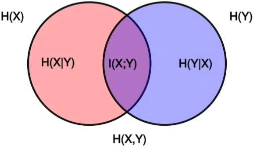
This can be thought of as the amount of uncertainty remaining in X after we learn the outcome of Y . We can now define the Mutual Information (Shannon, 1948) between X and Y , that is, the amount of information shared by X and Y , as follows:

I(X ;Y) = H(X)−H(X|Y)

=

∑

x∈Xy

∑

p(xy)log p(xy) p(x)p(y).

This is the difference of two entropies—the uncertainty before Y is known, H(X), and the uncer-tainty after Y is known, H(X|Y). This can also be interpreted as the amount of uncertainty in X which is removed by knowing Y , thus following the intuitive meaning of mutual information as the amount of information that one variable provides about another. It should be noted that the Mutual Information is symmetric, that is, I(X ;Y) =I(Y ; X), and is zero if and only if the variables are sta-tistically independent, that is p(xy) =p(x)p(y). The relation between these quantities can be seen in Figure 1. The Mutual Information can also be conditioned—the conditional information is,

I(X ;Y|Z) = H(X|Z)−H(X|Y Z)

=

∑

z∈Z

p(z)

∑

x∈Xy

∑

p(xy|z)log p(xy|z) p(x|z)p(y|z).

1. The base of the logarithm is arbitrary, but decides the ‘units’ of the entropy. When using base 2, the units are ‘bits’, when using base e, the units are ‘nats.’

Figure 1: Illustration of various information theoretic quantities.

This can be thought of as the information still shared between X and Y after the value of a third variable, Z, is revealed. The conditional mutual information will emerge as a particularly important property in understanding the results of this work.

This section has briefly covered the principles of information theory; in the following section we discuss motivations for using it to solve the feature selection problem.

2.2 Filter Criteria Based on Mutual Information

Filter methods are defined by a criterion J, also referred to as a ‘relevance index’ or ‘scoring’ criterion (Duch, 2006), which is intended to measure how potentially useful a feature or feature subset may be when used in a classifier. An intuitive J would be some measure of correlation between the feature and the class label—the intuition being that a stronger correlation between these should imply a greater predictive ability when using the feature. For a class label Y , the mutual information score for a feature Xk is

Jmim(Xk) =I(Xk;Y). (1)

been proposed that attempt to pursue this ‘relevancy-redundancy’ goal. For example, Battiti (1994) presents the Mutual Information Feature Selection (MIFS) criterion:

Jmi f s(Xk) =I(Xk;Y)−β

∑

I(Xk; Xj),

where S is the set of currently selected features. This includes the I(Xk;Y)term to ensure feature relevance, but introduces a penalty to enforce low correlations with features already selected in S. Note that this assumes we are selecting features sequentially, iteratively constructing our final feature subset. For a survey of other search methods than simple sequential selection, the reader is referred to Duch (2006); however it should be noted that all theoretical results presented in this paper will be generally applicable to any search procedure, and based solely on properties of the criteria themselves. The βin the MIFS criterion is a configurable parameter, which must be set experimentally. Using β=0 would be equivalent to Jmim(Xk), selecting features independently, while a larger value will place more emphasis on reducing inter-feature dependencies. In experi-ments, Battiti found thatβ=1 is often optimal, though with no strong theory to explain why. The MIFS criterion focuses on reducing redundancy; an alternative approach was proposed by Yang and Moody (1999), and also later by Meyer et al. (2008) using the Joint Mutual Information (JMI), to focus on increasing complementary information between features. The JMI score for feature Xkis

Jjmi(Xk) =

∑

I(XkXj;Y).

This is the information between the targets and a joint random variable XkXj, defined by pair-ing the candidate Xk with each feature previously selected. The idea is if the candidate feature is ‘complementary’ with existing features, we should include it.

The MIFS and JMI schemes were the first of many criteria that attempted to manage the relevance-redundancy tradeoff with various heuristic terms, however it is clear they have very dif-ferent motivations. The criteria identified in the literature 1992-2011 are listed in Table 1. The practice in this research problem has been to hand-design criteria, piecing criteria together as a jig-saw of information theoretic terms—the overall aim to manage the relevance-redundancy trade-off, with each new criterion motivated from a different direction. Several questions arise here: Which criterion should we believe? What do they assume about the data? Are there other useful criteria, as yet undiscovered? In the following section we offer a novel perspective on this problem.

3. A Novel Approach

In the following sections we formulate the feature selection task as a conditional likelihood problem. We will demonstrate that precise links can be drawn between the well-accepted statistical framework of likelihood functions, and the current feature selection heuristics of mutual information criteria.

3.1 A Conditional Likelihood Problem

Criterion Full name Authors

MIM Mutual Information Maximisation Lewis (1992)

MIFS Mutual Information Feature Selection Battiti (1994)

KS Koller-Sahami metric Koller and Sahami (1996)

JMI Joint Mutual Information Yang and Moody (1999)

MIFS-U MIFS-‘Uniform’ Kwak and Choi (2002)

IF Informative Fragments Vidal-Naquet and Ullman (2003)

FCBF Fast Correlation Based Filter Yu and Liu (2004)

AMIFS Adaptive MIFS Tesmer and Estevez (2004)

CMIM Conditional Mutual Info Maximisation Fleuret (2004)

MRMR Max-Relevance Min-Redundancy Peng et al. (2005)

ICAP Interaction Capping Jakulin (2005)

CIFE Conditional Infomax Feature Extraction Lin and Tang (2006)

DISR Double Input Symmetrical Relevance Meyer and Bontempi (2006)

MINRED Minimum Redundancy Duch (2006)

IGFS Interaction Gain Feature Selection El Akadi et al. (2008)

SOA Second Order Approximation Guo and Nixon (2009)

CMIFS Conditional MIFS Cheng et al. (2011)

Table 1: Various information-based criteria from the literature. Sections 3 and 4 will show how these can all be interpreted in a single theoretical framework.

irrelevant. Our modeling task is therefore two-fold: firstly to identify the features that play a func-tional role, and secondly to use these features to perform predictions. In this work we concentrate on the first stage, that of selecting the relevant features.

We adopt a d-dimensional binary vectorθ: a 1 indicating the feature is selected, a 0 indicating it is discarded. Notation x_θindicates the vector of selected features, that is, the full vector x projected onto the dimensions specified byθ. Notation x_eθis the complement, that is, the unselected features. The full feature vector can therefore be expressed as x={xθ,x_eθ}. As mentioned, we assume the process p is defined by a subset of the features, so for some unknown optimal vectorθ∗, we have that p(y|x) =p(y|x_θ∗). We approximate p using a hypothetical predictive model q, with two layers

of parameters: θrepresenting which features are selected, and τrepresenting parameters used to predict y. Our problem statement is to identify the minimal subset of features such that we maximize the conditional likelihood of the training labels, with respect to these parameters. For i.i.d. data

D

L

D

N

∏

i=1

q(yi|xi_θ,τ).

The (scaled) conditional log-likelihood is

ℓ= 1

N N

∑

i=1

log q(yi|xi_θ,τ). (2)

become popular in so-called discriminative modelling applications, where we are interested only in the classification performance; for example Grossman and Domingos (2004) used it to learn Bayesian Network classifiers. We will expand upon this link to discriminative models in Section 9.3. Maximising conditional likelihood corresponds to minimising KL-divergence between the true and predicted class posterior probabilities—for classification, we often only require the correct class, and not precise estimates of the posteriors, hence Equation (2) is a proxy lower bound for classification accuracy.

We now introduce the quantity p(y|x_θ): this is the true distribution of the class labels given the selected features x_θ. It is important to note the distinction from p(y|x), the true distribution given all features. Multiplying and dividing q by p(y|xθ), we can re-write the above as,

ℓ = 1

N N

∑

i=1

logq(y i_|xi

θ,τ)

p(yi_|xi

θ)

+ 1 N

N

∑

i=1

log p(yi|xi_θ). (3)

The second term in (3) can be similarly expanded, introducing the probability p(y|x):

ℓ = 1

N N

∑

i=1

logq(y i_|xi

θ,τ)

p(yi_|xi

θ)

+ 1 N

N

∑

i=1

logp(y i_|xi

θ)

p(yi_|xi₎ + 1 N

N

∑

i=1

log p(yi|xi).

These are finite sample approximations, drawing datapoints i.i.d. with respect to the distribution p(xy). We use Exy{·}to denote statistical expectation, and for convenience we negate the above, turning our maximisation problem into a minimisation. This gives us,

−ℓ ≈ Exy

n

log p(y|xθ) q(y|x_θ,τ)

o +Exy

n

log p(y|x) p(y|x_θ)

o −Exy

n

log p(y|x)o. (4)

These three terms have interesting properties which together define the feature selection prob-lem. It is particularly interesting to note that the second term is precisely that introduced by Koller and Sahami (1996) in their definitions of optimal feature selection. In their work, the term was adopted ad-hoc as a sensible objective to follow—here we have shown it to be a direct and nat-ural consequence of adopting the conditional likelihood as an objective function. Remembering

x={x_θ,x_eθ}, this second term can be developed:

∆KS = Exy

n

log p(y|x) p(y|x_θ)

o

=

∑

xy

p(xy)logp(y|xθxeθ) p(y|x_θ)

=

∑

xy

p(xy)logp(y|xθxeθ) p(y|x_θ)

p(x_eθ|x_θ) p(x_eθ|x_θ)

=

∑

xy

p(xy)log p(xeθy|xθ) p(x_eθ|xθ)p(y|xθ)

= I(X_eθ;Y|Xθ). (5)

quantity, the conditional entropy H(Y|X). In summary, we see that our objective function can be decomposed into three distinct terms, each with its own interpretation:

lim

N→∞−ℓ = Exy

n

log p(y|xθ) q(y|x_θ,τ)

o

+I(X_eθ;Y|X_θ) +H(Y|X). (6)

The first term is a likelihood ratio between the true and the predicted class distributions given the selected features, averaged over the input space. The size of this term will depend on how well the model q can approximate p, given the supplied features.3 Whenθtakes on the true valueθ∗(or consists of a superset ofθ∗) this becomes a KL-divergence p||q. The second term is I(X_eθ;Y|X_θ), the conditional mutual information between the class label and the unselected features, given the selected features. The size of this term depends solely on the choice of features, and will decrease as the selected feature set X_θ explains more about Y , until eventually becoming zero when the remaining features X_eθ contain no additional information about Y in the context of Xθ. It can be noted that due to the chain rule, we have

I(X ;Y) =I(X_θ;Y) +I(X_eθ;Y|X_θ),

hence minimizing I(X_eθ;Y|X_θ)is equivalent to maximising I(X_θ;Y). The final term is H(Y|X), the conditional entropy of the labels given all features. This term quantifies the uncertainty still remain-ing in the label even when we know all possible features; it is an irreducible constant, independent of all parameters, and in fact forms a bound on the Bayes error (Fano, 1961).

These three terms make explicit the effect of the feature selection parametersθ, separating them from the effect of the parametersτ in the model that uses those features. If we somehow had the optimal feature subsetθ∗, which perfectly captured the underlying process p, then I(X_eθ;Y|Xθ)would be zero. The remaining (reducible) error is then down to the KL divergence p||q, expressing how well the predictive model q can make use of the provided features. Of course, different models q will have different predictive ability: a good feature subset will not necessarily be put to good use if the model is too simple to express the underlying function. This perspective was also considered by Tsamardinos and Aliferis (2003), and earlier by Kohavi and John (1997)—the above results place these in the context of a precise objective function, the conditional likelihood. For the remainder of the paper we will use the same assumption as that made implicitly by all filter selection methods. For completeness, here we make the assumption explicit:

Definition 1 : Filter assumption

Given an objective function for a classifier, we can address the problems of optimizing the feature set and optimizing the classifier in two stages: first picking good features, then building the classifier to use them.

This implies that the second term in (6) can be optimized independently of the first. In this section we have formulated the feature selection task as a conditional likelihood problem. In the following, we consider how this problem statement relates to the existing literature, and discuss how to solve it in practice: including how to optimize the feature selection parameters, and the estimation of the necessary distributions.

3.2 Optimizing the Feature Selection Parameters

Under the filter assumption in Definition 1, Equation (6) demonstrates that the optima of the condi-tional likelihood coincide with that of the condicondi-tional mutual information:

arg max

θ

L

D

There may of course be multiple global optima, in addition to the trivial minimum of selecting all features. With this in mind, we can introduce a minimality constraint on the size of the feature set, and define our problem:

θ∗_{=arg min} θ′

{|θ′|:θ′=arg min

θ I(Xθ˜;Y|Xθ)}. (8)

This is the smallest feature set X_θ, such that the mutual information I(X_eθ;Y|X_θ) is minimal, and thus the conditional likelihood is maximal. It should be remembered that the likelihood is only our proxy for classification error, and the minimal feature set in terms of classification could be smaller than that which optimises likelihood. In the following paragraphs, we consider how this problem is implicitly tackled by methods already in the literature.

A common heuristic approach is a sequential search considering features one-by-one for ad-dition/removal; this is used for example in Markov Blanket learning algorithms such as IAMB (Tsamardinos et al., 2003). We will now demonstrate that this sequential search heuristic is in fact equivalent to a greedy iterative optimisation of Equation (8). To understand this we must time-index the feature sets. Notation X_θt/X_e

θt indicates the selected and unselected feature sets at timestep t—

with a slight abuse of notation treating these interchangeably as sets and random variables.

Definition 2 : Forward Selection Step with Mutual Information

The forward selection step adds the feature with the maximum mutual information in the context of the currently selected set X_θt. The operations performed are:

Xk = arg max Xk∈Xeθt

I(Xk;Y|Xθt),

X_θt+1 ← Xθt∪X_k,

X_eθt+1 ← X_eθt\Xk.

A subtle (but important) implementation point for this selection heuristic is that it should not add another feature if∀Xk, I(Xk;Y|Xθ) =0. This ensures we will not unnecessarily increase the size of the feature set.

Theorem 3 The forward selection mutual information heuristic adds the feature that generates the largest possible increase in the conditional likelihood—a greedy iterative maximisation.

Proof With the definitions above and the chain rule of mutual information, we have that:

I(X_eθt+1;Y|Xθt+1) =I(X_eθt;Y|Xθt)−I(Xk;Y|Xθt).

The feature Xk that maximises I(Xk;Y|Xθt) is the same that minimizes I(X_e

θt+1;Y|Xθt+1); therefore

Definition 4 : Backward Elimination Step with Mutual Information

In a backward step, a feature is removed—the utility of a feature Xk is considered as its mutual information with the target, conditioned on all other elements of the selected set without Xk. The operations performed are:

Xk = arg min Xk∈Xθt

I(Xk;Y|{Xθt\X_k}).

X_θt+1 ← Xθt\X_k

X_eθt+1 ← Xeθt∪Xk

Theorem 5 The backward elimination mutual information heuristic removes the feature that causes the minimum possible decrease in the conditional likelihood.

Proof With these definitions and the chain rule of mutual information, we have that:

I(X_eθt+1;Y|Xθt+1) =I(X_θet;Y|Xθt) +I(Xk;Y|Xθt+1).

The feature Xk that minimizes I(Xk;Y|X_θt+1)is that which keeps I(X_eθt+1;Y|Xθt+1) as close as

possi-ble to I(X_eθt;Y|Xθt); therefore the backward elimination step removes a feature while attempting to

maintain the likelihood as close as possible to its current value.

To strictly achieve our optimization goal, a backward step should only remove a feature if I(Xk;Y|{Xθt\X_k}) =0. In practice, working with real data, there will likely be estimation errors

(see the following section) and thus very rarely the strict zero will be observed. This brings us to an interesting corollary regarding IAMB (Tsamardinos and Aliferis, 2003).

Corollary 6 Since the IAMB algorithm uses precisely these forward/backward selection heuristics, it is a greedy iterative maximisation of the conditional likelihood. In IAMB, a backward elimination step is only accepted if I(Xk;Y|{Xθt\X_k})≈0, and otherwise the procedure terminates.

3.3 Estimation of the Mutual Information Terms

In considering the forward/backward heuristics, we must take account of the fact that we do not have perfect knowledge of the mutual information. This is because we have implicitly assumed we have access to the true distributions p(xy), p(y|x_θ), etc. In practice we have to estimate these from data. The problem calculating mutual information reduces to that of entropy estimation, and is fundamental in statistics (Paninski, 2003). The mutual information is defined as the expected logarithm of a ratio:

I(X ;Y) =Exy

n

log p(xy) p(x)p(y)

o

.

We can estimate this, since the Strong Law of Large Numbers assures us that the sample estimate using ˆp converges almost surely to the expected value—for a dataset of N i.i.d. observations(xi_,yi_),

I(X ;Y)≈_Iˆ_{(X ;Y) =} 1 N

N

∑

i=1

log pˆ(x i_yi₎

ˆ

p(xi_)pˆ(yi₎.

In order to calculate this we need the estimated distributions ˆp(xy), ˆp(x), and ˆp(y). The computation of entropies for continuous or ordinal data is highly non-trivial, and requires an assumed model of the underlying distributions—to simplify experiments throughout this article, we use discrete data, and estimate distributions with histogram estimators using fixed-width bins. The probability of any particular event p(X =x)is estimated by maximum likelihood, the frequency of occurrence of the event X =x divided by the total number of events (i.e., datapoints). For more information on alternative entropy estimation procedures, we refer the reader to Paninski (2003).

At this point we must note that the approximation above holds only if N is large relative to the dimension of the distributions over x and y. For example if x,y are binary, N ≈100 should be more than sufficient to get reliable estimates; however if x,y are multinomial, this will likely be insufficient. In the context of the sequential selection heuristics we have discussed, we are approximating I(Xk;Y|Xθ)as,

I(Xk;Y|Xθ)≈Iˆ(Xk;Y|Xθ) = 1 N

N

∑

i=1

log pˆ(x i kyi|xiθ) ˆ

p(xi_k|xi_θ)pˆ(yi_|xi

θ)

. (9)

As the dimension of the variable Xθ grows (i.e., as we add more features) then the necessary probability distributions become more high dimensional, and hence our estimate of the mutual information becomes less reliable. This in turn causes increasingly poor judgements for the in-clusion/exclusion of features. For precisely this reason, the research community have developed various low-dimensional approximations to (9). In the following sections, we will investigate the implicit statistical assumptions and empirical effects of these approximations.

In the remainder of this paper, we use I(X ;Y)to denote the ideal case of being able to compute the mutual information, though in practice on real data we use the finite sample estimate ˆI(X ;Y).

3.4 Summary

4. Retrofitting Successful Heuristics

In the previous section, starting from a clearly defined conditional likelihood problem, we derived a greedy optimization process which assesses features based on a simple scoring criterion on the utility of including a feature Xk∈Xe_θ. The score for a feature Xk is,

Jcmi(Xk) =I(Xk;Y|S), (10)

where cmi stands for conditional mutual information, and for notational brevity we now use S=Xθ

for the currently selected set. An important question is, how does (10) relate to existing heuristics in the literature, such as MIFS? We will see that MIFS, and certain other criteria, can be phrased cleanly as linear combinations of Shannon entropy terms, while some are non-linear combinations, involving max or min operations.

4.1 Criteria as Linear Combinations of Shannon Information Terms

Repeating the MIFS criterion for clarity,

Jmi f s(Xk) =I(Xk;Y)−β

∑

I(Xk; Xj). (11)

We can see that we first need to rearrange (10) into the form of a simple relevancy term between Xk and Y , plus some additional terms, before we can compare it to MIFS. Using the identity I(A; B|C)−

I(A; B) =I(A;C|B)−I(A;C), we can re-express (10) as,

Jcmi(Xk) =I(Xk;Y|S) =I(Xk;Y)−I(Xk; S) +I(Xk; S|Y). (12)

It is interesting to see terms in this expression corresponding to the concepts of ‘relevancy’ and ‘redundancy’, that is, I(Xk;Y) and I(Xk; S). The score will be increased if the relevancy of Xk is large and the redundancy with existing features is small. This is in accordance with a common view in the feature selection literature, observing that we wish to avoid redundant variables. However, we can also see an important additional term I(Xk; S|Y), which is not traditionally accounted for in the feature selection literature—we call this the conditional redundancy. This term has the opposite sign to the redundancy I(Xk; S), hence Jcmiwill be increased when this is large, that is, a strong class-conditional dependence of Xk with the existing set S. Thus, we come to the important conclusion that the inclusion of correlated features can be useful, provided the correlation within classes is stronger than the overall correlation. We note that this is a similar observation to that of Guyon et al. (2006), that “correlation does not imply redundancy”—Equation (12) effectively embodies this statement in information theoretic terms.

The sum of the last two terms in (12) represents the three-way interaction between the existing feature set S, the target Y , and the candidate feature Xk being considered for inclusion in S. To further understand this, we can note the following property:

I(XkS;Y) =I(S;Y) +I(Xk;Y|S) =I(S;Y) +I(Xk;Y)−I(Xk; S) +I(Xk; S|Y).

S combine well and provide more information together than by the sum of their parts, I(S;Y), and I(Xk;Y).

The important point to take away from this expression is that the terms are in a trade-off—we do not require a feature with low redundancy for its own sake, but instead require a feature that best trades off the three terms so as to maximise the score overall. Much like the bias-variance dilemma, attempting to decrease one term is likely to increase another.

The relation of (10) and (11) can be seen with assumptions on the underlying distribution p(xy). Writing the latter two terms of (12) as entropies:

Jcmi(Xk) = I(Xk;Y)

−H(S) +H(S|Xk)

+H(S|Y)−H(S|XkY). (13)

To develop this further, we require an assumption.

Assumption 1 For all unselected features Xk∈Xeθ, assume the following,

p(x_θ|xk) =

∏

p(xj|xk)

p(x_θ|xky) =

∏

p(xj|xky).

This states that the selected features X_θare independent and class-conditionally independent given the unselected feature Xkunder consideration.

Using this, Equation (13) becomes,

J_cmi′ (Xk) = I(Xk;Y)

−H(S) +

∑

j∈S

H(Xj|Xk)

+H(S|Y)−

∑

j∈S

H(Xj|XkY).

where the prime on J indicates we are making assumptions on the distribution. Now, if we introduce

∑j∈SH(Xj)−∑j∈SH(Xj), and∑j∈SH(Xj|Y)−∑j∈SH(Xj|Y), we recover mutual information terms, between the candidate feature and each member of the set S, plus some additional terms,

J_cmi′ (Xk) = I(Xk;Y)

−

∑

j∈S

I(Xj; Xk) +

∑

H(Xj)−H(S)

+

∑

j∈S

I(Xj; Xk|Y)−

∑

H(Xj|Y) +H(S|Y). (14)

Several of the terms in (14) are constant with respect to Xk—as such, removing them will have no effect on the choice of feature. Removing these terms, we have an equivalent criterion,

J_cmi′ (Xk) =I(Xk;Y)−

∑

I(Xj; Xk) +

∑

This has in fact already appeared in the literature as a filter criterion, originally proposed by Lin and Tang (2006), as Conditional Infomax Feature Extraction (CIFE), though it has been repeatedly rediscovered by other authors (El Akadi et al., 2008; Guo and Nixon, 2009). It is particularly interesting as it represents a sort of ‘root’ criterion, from which several others can be derived. For example, the link to MIFS can be seen with one further assumption, that the features are pairwise class-conditionally independent.

Assumption 2 For all features i,j, assume p(xixj|y) =p(xi|y)p(xj|y). This states that the features are pairwise class-conditionally independent.

With this assumption, the term ∑I(Xj; Xk|Y) will be zero, and (15) becomes (11), the MIFS criterion, withβ=1. Theβparameter in MIFS can be interpreted as encoding a strength of belief in another assumption, that of unconditional independence.

Assumption 3 For all features i,j, assume p(xixj) =p(xi)p(xj). This states that the features are pairwise independent.

Aβclose to zero implies very strong belief in the independence statement, indicating that any measured association I(Xj; Xk)is in fact spurious, possibly due to noise in the data. Aβvalue closer to 1 implies a lesser belief, that any measured dependency I(Xj; Xk)should be incorporated into the feature score exactly as observed. Since MIM is produced by settingβ=0, we can see that MIM also adopts Assumption 3. The same line of reasoning can be applied to a very similar criterion proposed by Peng et al. (2005), the Minimum-Redundancy Maximum-Relevance criterion,

Jmrmr(Xk) =I(Xk;Y)− 1

|S|

∑

Since mRMR omits the conditional redundancy term entirely, it is implicitly using Assumption 2. The β coefficient has been set inversely proportional to the size of the current feature set. If we have a large set S, thenβwill be extremely small. The interpretation is then that as the set S grows, mRMR adopts a stronger belief in Assumption 3. In the original paper, (Peng et al., 2005, Section 2.3) it was claimed that mRMR is equivalent to (10). In this section, through making explicit the intrinsic assumptions of the criterion, we have clearly illustrated that this claim is incorrect.

Balagani and Phoha (2010) present an analysis of the three criteria mRMR, MIFS and CIFE, arriving at similar results to our own: that these criteria make highly restrictive assumptions on the underlying data distributions. Though the conclusions are similar, our approach includes their results as a special case, and makes explicit the link to a likelihood function.

The relation of the MIFS/mRMR to Equation (15) is relatively straightforward. It is more chal-lenging to consider how closely other criteria might be re-expressed in this form. Yang and Moody (1999) propose using Joint Mutual Information (JMI),

Jjmi(Xk) =

∑

I(XkXj;Y). (16)

Using some relatively simple manipulations (see appendix) this can be re-written as,

Jjmi(Xk) =I(Xk;Y)− 1

|S|

∑

I(Xk; Xj)−I(Xk; Xj|Y)

i

This criterion (17) returns exactly the same set of features as the JMI criterion (16); however in this form, we can see the relation to our proposed framework. The JMI criterion, like mRMR, has a stronger belief in the pairwise independence assumptions as the feature set S grows. Similarities can of course be observed between JMI, MIFS and mRMR—the differences being the scaling factor and the conditional term—and their subsequent relation to Equation (15). It is in fact possible to identify numerous criteria from the literature that can all be re-written into a common form, corresponding to variations upon (15). A space of potential criteria can be imagined, where we parameterize criterion (15) as so:

J_cmi′ =I(Xk;Y)−β

∑

I(Xj; Xk) +γ

∑

I(Xj; Xk|Y). (18)

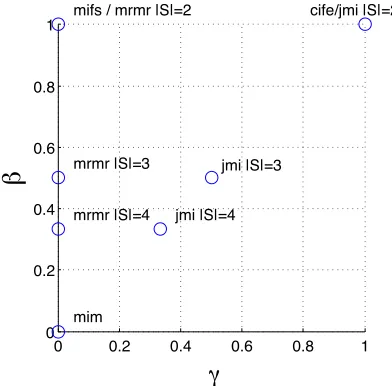
Figure 2 shows how the criteria we have discussed so far can all be fitted inside this unit square corresponding toβ/γparameters. MIFS sits on the left hand axis of the square—with γ=0 and

β∈[0,1]. The MIM criterion, Equation (1), which simply assesses each feature individually without any regard of others, sits at the bottom left, withγ=0,β=0. The top right of the square corresponds toγ=1,β=1, which is the CIFE criterion (Lin and Tang, 2006), also suggested by El Akadi et al. (2008) and Guo and Nixon (2009). A very similar criterion, using an assumption to approximate the terms, was proposed by Cheng et al. (2011).

The JMI and mRMR criteria are unique in that they move linearly within the space as the feature set S grows. As the size of the set S increases they move closer towards the origin and the MIM criterion. The particularly interesting point about this property is that the relative magnitude of the relevancy term to the redundancy terms stays approximately constant as S grows, whereas with MIFS, the redundancy term will in general be|S|times bigger than the relevancy term. The conse-quences of this will be explored in the experimental section of this paper. Any criterion expressible in the unit square has made independence Assumption 1. In addition, any criteria that sit at points other thanβ=1,γ=1 have adopted varying degrees of belief in Assumptions 2 and 3.

A further interesting point about this square is simply that it is sparsely populated. An obvious unexplored region is the bottom right, the corner corresponding to β=0,γ=1; though there is no clear intuitive justification for this point, for completeness in the experimental section we will evaluate it, as the conditional redundancy or ‘condred’ criterion. In previous work (Brown, 2009) we explored this unit square, though derived from an expansion of the mutual information function rather than directly from the conditional likelihood. While this resulted in an identical expression to (18), the probabilistic framework we present here is far more expressive, allowing exact specifi-cation of the underlying assumptions.

The unit square of Figure 2 describes linear criteria, named as so since they are linear combi-nations of the relevance/redundancy terms. There exist other criteria that follow a similar form, but involving other operations, making them non-linear.

4.2 Criteria as Non-Linear Combinations of Shannon Information Terms

Fleuret (2004) proposed the Conditional Mutual Information Maximization criterion,

Jcmim(Xk) =min Xj∈S

h

I(Xk;Y|Xj)

i

.

This can be re-written,

Jcmim(Xk) =I(Xk;Y)−max Xj∈S

h

I(Xk; Xj)−I(Xk; Xj|Y)

i

Figure 2: The full space of linear filter criteria, describing several examples from Table 1. Note that all criteria in this space adopt Assumption 1. Additionally, theγandβaxes represent the criteria belief in Assumptions 2 and 3, respectively. The left hand axis is where the mRMR and MIFS algorithms sit. The bottom left corner, MIM, is the assumption of completely independent features, using just marginal mutual information. Note that some criteria are equivalent at particular sizes of the current feature set|S|.

The proof is again available in the appendix. Due to the max operator, the probabilistic interpretation is a little less straightforward. It is clear however that CMIM adopts Assumption 1, since it evaluates only pairwise feature statistics.

Vidal-Naquet and Ullman (2003) propose another criterion used in Computer Vision, which we refer to as Informative Fragments,

Ji f(Xk) =min Xj∈S

h

I(XkXj;Y)−I(Xj;Y)

i

.

The authors motivate this criterion by noting that it measures the gain of combining a new feature Xk with each existing feature Xj, over simply using Xj by itself. The Xj with the least ‘gain’ from being paired with Xk is taken as the score for Xk. Interestingly, using the chain rule I(XkXj;Y) = I(Xj;Y) +I(Xk;Y|Xj), therefore IF is equivalent to CMIM, that is, Ji f(Xk) =Jcmim(Xk), making the same assumptions. Jakulin (2005) proposed the criterion,

Jicap(Xk) =I(Xk;Y)−

∑

max

h

0,{I(Xk; Xj)−I(Xk; Xj|Y)}

i

.

Again, this adopts Assumption 1, using the same redundancy and conditional redundancy terms, yet the exact probabilistic interpretation is unclear.

Symmetrical Relevance (Meyer and Bontempi, 2006), a modification of the JMI criterion:

Jdisr(Xk) =

∑

I(XkXj;Y) H(XkXjY)

.

The inclusion of this normalisation term breaks the strong theoretical link to a likelihood function, but again for completeness we will include this in our empirical investigations. While the criteria in the unit square can have their probabilistic assumptions made explicit, the nonlinearity in the CMIM, ICAP and DISR criteria make such an interpretation far more difficult.

4.3 Summary of Theoretical Findings

In this section we have shown that numerous criteria published over the past two decades of research can be ‘retro-fitted’ into the framework we have proposed—the criteria are approximations to (10), each making different assumptions on the underlying distributions. Since in the previous section we saw that accepting the top ranked feature according to (10) provides the maximum possible increase in the likelihood, we see now that the criteria are approximate maximisers of the likelihood. Whether or not they indeed provide the maximum increase at each step will depend on how well the implicit assumptions on the data can be trusted. Also, it should be remembered that even if we used (10), it is not guaranteed to find the global optimum of the likelihood, since (a) it is a greedy search, and (b) finite data will mean distributions cannot be accurately modelled. In this case, we have reached the limit of what a theoretical analysis can tell us about the criteria, and we must close the remaining ‘gaps’ in our understanding with an experimental study.

5. Experiments

In this section we empirically evaluate some of the criteria in the literature against one another. Note that we are not pursuing an exhaustive analysis, attempting to identify the ‘winning’ criterion that provides best performance overall4—rather, we primarily observe how the theoretical properties of criteria relate to the similarity of the returned feature sets. While these properties are interest-ing, we of course must acknowledge that classification performance is the ultimate evaluation of a criterion—hence we also include here classification results on UCI data sets and in Section 6 on the well-known benchmark NIPS Feature Selection Challenge.

In the following sections, we ask the questions: “how stable is a criterion to small changes in the training data set?”, “how similar are the criteria to each other?”, “how do the different criteria behave in limited and extreme small-sample situations?”, and finally, “what is the relation between stability and accuracy?”.

To address these questions, we use the 15 data sets detailed in Table 2. These are chosen to have a wide variety of example-feature ratios, and a range of multi-class problems. The features within each data set have a variety of characteristics—some binary/discrete, and some continuous. Con-tinuous features were discretized, using an equal-width strategy into 5 bins, while features already with a categorical range were left untouched. The ‘ratio’ statistic quoted in the final column is an indicator of the difficulty of the feature selection for each data set. This uses the number of data-points (N), the median arity of the features (m), and the number of classes (c)—the ratio quoted in

the table for each data set is_mcN, hence a smaller value indicates a more challenging feature selection problem.

A key point of this work is to understand the statistical assumptions on the data imposed by the feature selection criteria—if our classification model were to make even more assumptions, this is likely to obscure the experimental observations relating performance to theoretical properties. For this reason, in all experiments we use a simple nearest neighbour classifier (k=3), this is chosen as it makes few (if any) assumptions about the data, and we avoid the need for parameter tuning. For the feature selection search procedure, the filter criteria are applied using a simple forward selection, to select a fixed number of features, specified in each experiment, before being used with the classifier.

Data Features Examples Classes Ratio

breast 30 569 2 57

congress 16 435 2 72

heart 13 270 2 34

ionosphere 34 351 2 35

krvskp 36 3196 2 799

landsat 36 6435 6 214

lungcancer 56 32 3 4

parkinsons 22 195 2 20

semeion 256 1593 10 80

sonar 60 208 2 21

soybeansmall 35 47 4 6

spect 22 267 2 67

splice 60 3175 3 265

waveform 40 5000 3 333

wine 13 178 3 12

Table 2: Data sets used in experiments. The final column indicates the difficulty of the data in feature selection, a smaller value indicating a more challenging problem.

5.1 How Stable are the Criteria to Small Changes in the Data?

for this, Kuncheva (2007) presents a consistency index, based on the hypergeometric distribution with a correction for chance.

Definition 7 The consistency for two subsets A,B⊂X , such that |A|=|B|=k, and r=|A∩B|, where 0<k<|X|=n, is

C(A,B) = rn−k 2 k(n−k).

The consistency takes values in the range [−1,+1], with a positive value indicating similar sets, a zero value indicating a purely random relation, and a negative value indicating a strong anti-correlation between the features sets.

One problem with the consistency index is that it does not take feature redundancy into account. That is, two procedures could select features which have different array indices, so are identified as ‘different’, but in fact are so highly correlated that they are effectively identical. A method to deal with this situation was proposed by Yu et al. (2008). This method constructs a weighted complete bipartite graph, where the two node sets correspond to two different feature sets, and weights are assigned to the arcs are the normalized mutual information between the features at the nodes, also sometimes referred to as the symmetrical uncertainty. The weight between node i in set A, and node

j in set B, is

w(A(i),B(j)) = I(XA(i); XB(j)) H(XA(i)) +H(XB(j))

.

The Hungarian algorithm is then applied to identify the maximum weighted matching between the two node sets, and the overall similarity between sets A and B is the final matching cost. This is the information consistency of the two sets. For more details, we refer to Yu et al. (2008).

We now compare these two measures on the criteria from the previous sections. For each data set, we take a bootstrap sample and select a set of features using each feature selection criterion. The (information) stability of a single criterion is quantified as the average pairwise (information) consistency across 50 bootstraps from the training data.

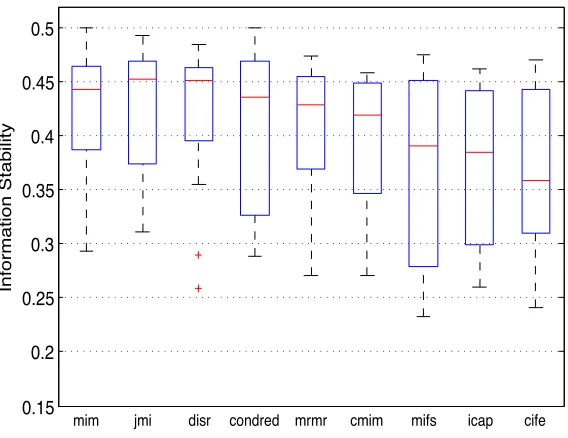
Figure 3 shows Kuncheva’s stability measure on average over 15 data sets, selecting feature sets of size 10; note that the criteria have been displayed ordered left-to-right by their median value of stability over the 15 data sets. The marginal mutual information, MIM, is as expected the most stable, given that it has the lowest dimensional distribution to approximate. The next most stable is JMI which includes the relevancy/redundancy terms, but averages over the current feature set; this averaging process might therefore be interpreted empirically as a form of ‘smoothing’, enabling the criteria overall to be resistant to poor estimation of probability distributions. It can be noted that the far right of Figure 3 consists of the MIFS, ICAP and CIFE criteria, all of which do not attempt to average the redundancy terms.

Figure 3: Kuncheva’s Stability Index across 15 data sets. The box indicates the upper/lower quar-tiles, the horizontal line within each shows the median value, while the dotted crossbars indicate the maximum/minimum values. For convenience of interpretation, criteria on the x-axis are ordered by their median value.

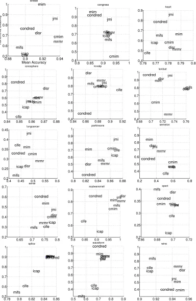
(a) Kuncheva’s Consistency Index. (b) Yu et al’s Information Stability Index.

Figure 5: Relations between feature sets generated by different criteria, on average over 15 data sets. 2-D visualisation generated by classical multi-dimensional scaling.

5.2 How Similar are the Criteria?

Two criteria can be directly compared with the same methodology: by measuring the consistency and information consistency between selected feature subsets on a common set of data. We calculate the mean consistencies between two feature sets of size 10, repeatedly selected over 50 bootstraps from the original data. This is then arranged in a similarity matrix, and we use classical multi-dimensional scaling to visualise this as a 2-d map, shown in Figures 5a and 5b. Note again that while the indices may return different absolute values (one is a normalized mean of a hypergeometric distribution and the other is a pairwise sum of mutual information terms) they show very similar relative ‘distances’ between criteria.

5.3 How do Criteria Behave in Limited and Extreme Small-sample Situations?

To assess how criteria behave in data poor situations, we vary the number of datapoints supplied to perform the feature selection. The procedure was to randomly select 140 datapoints, then use the remaining data as a hold-out set. From this 140, the number provided to each criterion was increased in steps of 10, from a minimal set of size 20. To allow a reasonable testing set size, we limited this assessment to only data sets with at least 200 datapoints total; this gives us 11 data sets from the 15, omitting lungcancer, parkinsons, soybeansmall, and wine. For each data set we select 10 features and apply the 3-nn classifier, recording the rank-order of the criteria in terms of their generalisation error. This process was repeated and averaged over 50 trials, giving the results in Figure 6.

To aid interpretation we label MIM with a simple point marker, MIFS, CIFE, CondRed, and ICAP with a circle, and the remaining criteria (DISR, JMI, mRMR and CMIM) with a star. The criteria labelled with a star balance the relative magnitude of the relevancy and redundancy terms, those with a circle do not attempt to balance them, and MIM contains no redundancy term. There is a clear separation between those criteria with a star outperforming those with a circle, and MIM varying in performance between the two groups as we allow more training datapoints.

Notice that the highest ranked criteria coincide with those in the cluster at the top left of Figures 5a and 5b. We suggest that the relative difference in performance is due to the same reason noted in Section 5.2, that the redundancy term grows with the size of the selected feature set. In this case, the redundancy term eventually grows to outweigh the relevancy by a large degree, and the new features are selected solely on the basis of redundancy, ignoring the relevance, thus leading to poor classification performance.

20 40 60 80 100 120 140

1 2 3 4 5 6 7 8 9

Training points

Rank

mim mifs condred cife icap mrmr jmi disr cmim

Data Features Examples Classes

Colon 2000 62 2

Leukemia 7070 72 2

Lung 325 73 7

Lymph 4026 96 9

NCI9 9712 60 9

Table 3: Data sets from Peng et al. (2005), used in experiments.

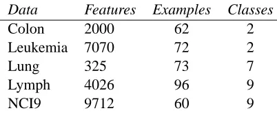
5.4 Extreme Small-Sample Experiments

In the previous sections we discussed two theoretical properties of information-based feature se-lection criteria: whether it balances the relative magnitude of relevancy against redundancy, and whether it includes a class-conditional redundancy term. Empirically on the UCI data sets, we see that the balancing is far more important than the inclusion of the conditional redundancy term—for example, MRMR succeeds in many cases, while MIFS performs poorly. Now, we consider whether same property may hold in extreme small-sample situations, when the number of examples is so low that reliable estimation of distributions becomes extremely difficult. We use data sourced from Peng et al. (2005), detailed in Table 3. Results are shown in Figure 7, selecting 50 features from each data set and plotting leave-one-out classification error. It should of course be remembered that on such small data sets, making just one additional datapoint error can result in seemingly large changes in accuracy. For example, the difference between the best and worst criteria on Leukemia was just 3 datapoints. In contrast to the UCI results, the picture is less clear. On Colon, the criteria all perform similarly; this is the least complex of all the data sets, having the smallest number of classes with a (relatively) small number of features. As we move through the data sets with in-creasing numbers of features/classes, we see that MIFS, CONDRED, CIFE and ICAP start to break away, performing poorly compared to the others. Again, we note that these do not attempt to bal-ance relevancy/redundancy. This difference is clearest on the NCI9 data, the most complex with 9 classes and 9712 features. However, as we may expect with such high dimensional and challenging problems, there are some exceptions—the Colon data as mentioned, and also the Lung data where ICAP/MIFS perform well.

5.5 What is the Relation Between Stability and Accuracy?

An important question is whether we can find a good balance between the stability of a criterion and the classification accuracy. This was considered by Gulgezen et al. (2009), who studied the sta-bility/accuracy trade-off for the MRMR criterion. In the following, we consider this trade-off in the context of Pareto-optimality, across the 9 criteria, and the 15 data sets from Table 2. Experimental protocol was to take 50 bootstraps from the data set, each time calculating the out-of-bag error using the 3-nn. The stability measure was Kuncheva’s stability index calculated from the 50 feature sets, and the accuracy was the mean out-of-bag accuracy across the 50 bootstraps. The experiments were also repeated using the Information Stability measure, revealing almost identical results. Results using Kuncheva’s stability index are shown in Figure 8.

0 5 10 15 20 25 30 35 40 45 50 0 5 10 15 20 25 30 35 40 45 Colon

Number of features selected

LOO number of mistakes

mim mifs condred cife icap mrmr jmi disr cmim

0 5 10 15 20 25 30 35 40 45 50 0

5 10 15

Leukemia

Number of features selected

LOO number of mistakes

0 5 10 15 20 25 30 35 40 45 50 0 5 10 15 20 25 30 35 40 45 50 Lung

Number of features selected

LOO number of mistakes

0 5 10 15 20 25 30 35 40 45 50 0 5 10 15 20 25 30 35 40 45 50 Lymphoma

Number of features selected

LOO number of mistakes

0 5 10 15 20 25 30 35 40 45 50 20 25 30 35 40 45 50 55 NCI9

Number of features selected

LOO number of mistakes

Accuracy/Stability(Yu) Accuracy/Stability(Kuncheva) Accuracy

JMI (1.6) JMI (1.5) JMI (2.6)

DISR (2.3) DISR (2.2) MRMR (3.6)

MIM (2.4) MIM (2.3) DISR (3.7)

MRMR (2.5) MRMR (2.5) CMIM (4.5)

CMIM (3.3) CONDRED (3.2) ICAP (5.3)

ICAP (3.6) CMIM (3.4) MIM (5.4)

CONDRED (3.7) ICAP (4.3) CIFE (5.9)

CIFE (4.3) CIFE (4.8) MIFS (6.5)

MIFS (4.5) MIFS (4.9) CONDRED (7.4)

Table 4: Column 1: Non-dominated Rank of different criteria for the trade-off of accuracy/stability. Criteria with a higher rank (closer to 1.0) provide a better tradeoff than those with a lower rank. Column 2: As column 1 but using Kuncheva’s Stability Index. Column 3: Average ranks for accuracy alone.

that appear further to the top-right of the space dominate those toward the bottom left—in such a situation there is no reason to choose those at the bottom left, since they are dominated on both objectives by other criteria.

A summary (for both stability and information stability) is provided in the first two columns of Table 4, showing the non-dominated rank of the different criteria. This is computed per data set as the number of other criteria which dominate a given criterion, in the Pareto-optimal sense, then averaged over the 15 data sets. We can see that these rankings are similar to the results earlier, with MIFS, ICAP, CIFE and CondRed performing poorly. We note that JMI, (which both balances the relevancy and redundancy terms and includes the conditional redundancy) outperforms all other criteria.

JMI

MRMR

ICAP DISR

CMIM

CIFE

MIFS

CONDRED MIM

99% Confidence 95% Confidence 90% Confidence

5.6 Summary of Empirical Findings

From experiments in this section, we conclude that the balance of relevancy/redundancy terms is extremely important, while the inclusion of a class conditional term seems to matter less. We find that some criteria are inherently more stable than others, and that the trade-off between accuracy (using a simple k-nn classifier) and stability of the feature sets differs between criteria. The best overall trade-off for accuracy/stability was found in the JMI and MRMR criteria. In the following section we re-assess these findings, in the context of two problems posed for the NIPS Feature Selection Challenge.

6. Performance on the NIPS Feature Selection Challenge

In this section we investigate performance of the criteria on data sets taken from the NIPS Feature Selection Challenge (Guyon, 2003).

6.1 Experimental Protocols

We present results using GISETTE (a handwriting recognition task), and MADELON (an artificially generated data set).

Data Features Examples (Tr/Val) Classes

GISETTE 5000 6000/1000 2

MADELON 500 2000/600 2

Table 5: Data sets from the NIPS challenge, used in experiments.

To apply the mutual information criteria, we estimate the necessary distributions using his-togram estimators: features were discretized independently into 10 equal width bins, with bin boundaries determined from training data. After the feature selection process the original (undis-cretised) data sets were used to classify the validation data. Each criterion was used to generate a ranking for the top 200 features in each data set. We show results using the full top 200 for GISETTE, but only the top 20 for MADELON as after this point all criteria demonstrated severe overfitting. We use the Balanced Error Rate, for fair comparison with previously published work on the NIPS data sets. We accept that this does not necessarily share the same optima as the classifi-cation error (to which the conditional likelihood relates), and leave investigations of this to future work.

Validation data results are presented in Figure 10 (GISETTE) and Figure 11 (MADELON). The minimum of the validation error was used to select the best performing feature set size, the training data alone used to classify the testing data, and finally test labels were submitted to the challenge website. Test results are provided in Table 6 for GISETTE, and Table 7 for MADELON.5

Unlike in Section 5, the data sets we have used from the NIPS Feature Selection Challenge have a greater number of datapoints (GISETTE has 6000 training examples, MADELON has 2000) and thus we can present results using a direct implementation of Equation (10) as a criterion. We refer to this criterion as CMI, as it is using the conditional mutual information to score features. Unfortunately there are still estimation errors in this calculation when selecting a large number of

0 20 40 60 80 100 120 140 160 180 200 0

0.05 0.1 0.15 0.2 0.25 0.3 0.35 0.4 0.45 0.5

Number of Features

Validation Error

cmi mim mifs cife icap mrmr jmi disr cmim

Figure 10: Validation Error curve using GISETTE.

0 2 4 6 8 10 12 14 16 18 20

0 0.05 0.1 0.15 0.2 0.25 0.3 0.35 0.4 0.45 0.5

Number of Features

Validation Error

cmi mim mifs cife icap mrmr jmi disr cmim

features, even given the large number of datapoints and so the criterion fails to select features after a certain point, as each feature appears equally irrelevant. In GISETTE, CMI selected 13 features, and so the top 10 features were used and thus one result is shown. In MADELON, CMI selected 7 features and so 7 results are shown.

6.2 Results on Test Data

In Table 6 there are several distinctions between the criteria, the most striking of which is the failure of MIFS to select an informative feature set. The importance of balancing the magnitude of the relevancy and the redundancy can be seen whilst looking at the other criteria in this test. Those criteria which balance the magnitudes, (CMIM, JMI, & mRMR) perform better than those which do not (ICAP,CIFE). The DISR criterion forms an outlier here as it performs poorly when compared to JMI. The only difference between these two criteria is the normalization in DISR—as such, this is the likely cause of the observed poor performance, the introduction of more variance by estimating the normalization H(XkXjY).

We can also see how important the low dimensional approximation is, as even with 6000 training examples CMI cannot estimate the required joint distribution to avoid selecting probes, despite being a direct iterative maximisation of the conditional likelihood in the limit of datapoints.

Criterion BER AUC Features (%) Probes (%)

MIM 4.18 95.82 4.00 0.00

MIFS 42.00 58.00 4.00 58.50

CIFE 6.85 93.15 2.00 0.00

ICAP 4.17 95.83 1.60 0.00

CMIM 2.86 97.14 2.80 0.00

CMI 8.06 91.94 0.20 20.00

mRMR 2.94 97.06 3.20 0.00

JMI 3.51 96.49 4.00 0.00

DISR 8.03 91.97 4.00 0.00

Winning Challenge Entry 1.35 98.71 18.3 0.0

Table 6: NIPS FS Challenge Results: GISETTE.

The MADELON results (Table 7) show a particularly interesting point—the top performers (in terms of BER) are JMI and CIFE. Both these criteria include the class-conditional redundancy term, but CIFE does not balance the influence of relevancy against redundancy. In this case, it appears the ‘balancing’ issue, so important in our previous experiments seems to have little importance— instead, the presence of the conditional redundancy term is the differentiating factor between criteria (note the poor performance of MIFS/MRMR). This is perhaps not surprising given the nature of the MADELON data, constructed precisely to require features to be evaluated jointly.

It is interesting to note that the challenge organisers benchmarked a 3-NN using the optimal feature set, achieving a 10% test error (Guyon, 2003). Many of the criteria managed to select feature sets which achieved a similar error rate using a 3-NN, and it is likely that a more sophisticated classifier is required to further improve performance.