Communication-Efficient Algorithms for Statistical Optimization
Yuchen Zhang [email protected]
John C. Duchi [email protected]
Department of Electrical Engineering and Computer Sciences University of California, Berkeley
Berkeley, CA 94720 USA
Martin J. Wainwright [email protected]
Department of Statistics
University of California, Berkeley Berkeley, CA 94720 USA
Editor: Francis Bach
Abstract
We analyze two communication-efficient algorithms for distributed optimization in statistical set-tings involving large-scale data sets. The first algorithm is a standard averaging method that distributes the N data samples evenly to m machines, performs separate minimization on each subset, and then averages the estimates. We provide a sharp analysis of this average mixture algorithm, showing that under a reasonable set of conditions, the combined parameter achieves mean-squared error (MSE) that decays asO(N−1+ (N/m)−2). Whenever m≤√N, this guaran-tee matches the best possible rate achievable by a centralized algorithm having access to all N samples. The second algorithm is a novel method, based on an appropriate form of bootstrap subsampling. Requiring only a single round of communication, it has mean-squared error that decays as O(N−1+ (N/m)−3), and so is more robust to the amount of parallelization. In ad-dition, we show that a stochastic gradient-based method attains mean-squared error decaying as O(N−1+ (N/m)−3/2), easing computation at the expense of a potentially slower MSE rate. We also provide an experimental evaluation of our methods, investigating their performance both on simulated data and on a large-scale regression problem from the internet search domain. In particu-lar, we show that our methods can be used to efficiently solve an advertisement prediction problem from the Chinese SoSo Search Engine, which involves logistic regression with N≈2.4×10⁸ sam-ples and d≈740,000 covariates.
Keywords: distributed learning, stochastic optimization, averaging, subsampling
1. Introduction
single computer, or at least to keep the data in memory. Accordingly, the focus of this paper is the study of some distributed and communication-efficient procedures for empirical risk minimization. Recent years have witnessed a flurry of research on distributed approaches to solving very large-scale statistical optimization problems. Although we cannot survey the literature adequately—the papers Nedi´c and Ozdaglar (2009), Ram et al. (2010), Johansson et al. (2009), Duchi et al. (2012a), Dekel et al. (2012), Agarwal and Duchi (2011), Recht et al. (2011), Duchi et al. (2012b) and ref-erences therein contain a sample of relevant work—we touch on a few important themes here. It can be difficult within a purely optimization-theoretic setting to show explicit benefits arising from distributed computation. In statistical settings, however, distributed computation can lead to gains in computational efficiency, as shown by a number of authors (Agarwal and Duchi, 2011; Dekel et al., 2012; Recht et al., 2011; Duchi et al., 2012b). Within the family of distributed algorithms, there can be significant differences in communication complexity: different computers must be synchronized, and when the dimensionality of the data is high, communication can be prohibitively expensive. It is thus interesting to study distributed estimation algorithms that require fairly limited synchroniza-tion and communicasynchroniza-tion while still enjoying the greater statistical accuracy that is usually associated with a larger data set.
With this context, perhaps the simplest algorithm for distributed statistical estimation is what we term the average mixture (AVGM) algorithm. It is an appealingly simple method: given m different machines and a data set of size N, first assign to each machine a (distinct) data set of size n=N/m, then have each machine i compute the empirical minimizerθion its fraction of the data, and finally average all the parameter estimatesθiacross the machines. This approach has been studied for some classification and estimation problems by Mann et al. (2009) and McDonald et al. (2010), as well as for certain stochastic approximation methods by Zinkevich et al. (2010). Given an empirical risk minimization algorithm that works on one machine, the procedure is straightforward to implement and is extremely communication efficient, requiring only a single round of communication. It is also relatively robust to possible failures in a subset of machines and/or differences in speeds, since there is no repeated synchronization. When the local estimators are all unbiased, it is clear that the the AVGMprocedure will yield an estimate that is essentially as good as that of an estimator based on all N samples. However, many estimators used in practice are biased, and so it is natural to ask whether the method has any guarantees in a more general setting. To the best of our knowledge, however, no work has shown rigorously that the AVGMprocedure generally has greater efficiency than the naive approach of using n=N/m samples on a single machine.
This paper makes three main contributions. First, in Section 3, we provide a sharp analysis of the AVGM algorithm, showing that under a reasonable set of conditions on the population risk, it can indeed achieve substantially better rates than the naive approach. More concretely, we provide bounds on the mean-squared error (MSE) that decay as
O
((nm)−1+n−2). Whenever the number of machines m is less than the number of samples n per machine, this guarantee matches the best possible rate achievable by a centralized algorithm having access to all N =nm samples. In the special case of optimizing log likelihoods, the pre-factor in our bound involves the trace of the Fisher information, a quantity well-known to control the fundamental limits of statistical estimation. We also show how the result extends to stochastic programming approaches, exhibiting a stochastic gradient-descent based procedure that also attains convergence rates scaling asO
((nm)−1), but with slightly worse dependence on different problem-specific parameters.we refer to as the subsampled average mixture (SAVGM) approach. At a high level, the SAVGM
algorithm distributes samples evenly among m processors or computers as before, but instead of simply returning the empirical minimizer, each processor further subsamples its own data set in order to estimate the bias of its own estimate, and returns a subsample-corrected estimate. We establish that the SAVGMalgorithm has mean-squared error decaying as
O
(m−1n−1+n−3). As long as m<n2, the subsampled method again matches the centralized gold standard in the first-order term, and has a second-order term smaller than the standard averaging approach.Our third contribution is to perform a detailed empirical evaluation of both the AVGM and SAVGM procedures, which we present in Sections 4 and 5. Using simulated data from normal and non-normal regression models, we explore the conditions under which the SAVGMalgorithm yields
better performance than the AVGMalgorithm; in addition, we study the performance of both meth-ods relative to an oracle baseline that uses all N samples. We also study the sensitivity of the algo-rithms to the number of splits m of the data, and in the SAVGMcase, we investigate the sensitivity of
the method to the amount of resampling. These simulations show that both AVGMand SAVGMhave favourable performance, even when compared to the unattainable “gold standard” procedure that has access to all N samples. In Section 5, we complement our simulation experiments with a large logistic regression experiment that arises from the problem of predicting whether a user of a search engine will click on an advertisement. This experiment is large enough—involving N≈2.4×10⁸ samples in d≈740,000 dimensions with a storage size of approximately 55 gigabytes—that it is difficult to solve efficiently on one machine. Consequently, a distributed approach is essential to take full advantage of this data set. Our experiments on this problem show that SAVGM—with the resampling and correction it provides—gives substantial performance benefits over naive solutions as well as the averaging algorithm AVGM.
2. Background and Problem Set-up
We begin by setting up our decision-theoretic framework for empirical risk minimization, after which we describe our algorithms and the assumptions we require for our main theoretical results.
2.1 Empirical Risk Minimization
Let{f(·; x),x∈
X
}be a collection of real-valued and convex loss functions, each defined on a set containing the convex set Θ⊆Rd. Let P be a probability distribution over the sample spaceX
. Assuming that each function x7→ f(θ; x)is P-integrable, the population risk F0:Θ→Ris given byF0(θ):=EP[f(θ; X)] =
Z
X
f(θ; x)dP(x).
Our goal is to estimate the parameter vector minimizing the population risk, namely the quantity
θ∗:=argmin θ∈Θ
F0(θ) =argmin
θ∈Θ
Z
X f
(θ; x)dP(x),
which we assume to be unique. In practice, the population distribution P is unknown to us, but we have access to a collection S of samples from the distribution P. Empirical risk minimization is based on estimatingθ∗by solving the optimization problem
b
θ∈argmin
θ∈Θ n 1
|S|x
∑
∈Sf(θ; x)Throughout the paper, we impose some regularity conditions on the parameter space, the risk function F0, and the instantaneous loss functions f(·; x):Θ→R. These conditions are standard in classical statistical analysis of M-estimators (e.g., Lehmann and Casella, 1998; Keener, 2010). Our first assumption deals with the relationship of the parameter space to the optimal parameterθ∗.
Assumption 1 (Parameters) The parameter spaceΘ⊂Rdis a compact convex set, withθ∗∈intΘ andℓ2-radius R=max
θ∈Θkθ−θ ∗k
2.
In addition, the risk function is required to have some amount of curvature. We formalize this notion in terms of the Hessian of F0:
Assumption 2 (Local strong convexity) The population risk is twice differentiable, and there
ex-ists a parameterλ>0 such that∇2F0(θ∗)λId×d.
Here∇2F0(θ)denotes the d×d Hessian matrix of the population objective F0evaluated atθ, and we use to denote the positive semidefinite ordering (i.e., AB means that A−B is positive semidefinite.) This local condition is milder than a global strong convexity condition and is required to hold only for the population risk F0 evaluated atθ∗. It is worth observing that some type of curvature of the risk is required for any method to consistently estimate the parametersθ∗.
2.2 Averaging Methods
Consider a data set consisting of N=mn samples, drawn i.i.d. according to the distribution P. In the distributed setting, we divide this N-sample data set evenly and uniformly at random among a total of m processors. (For simplicity, we have assumed the total number of samples is a multiple of m.) For i=1, . . . ,m, we let S1,i denote the data set assigned to processor i; by construction, it
is a collection of n samples drawn i.i.d. according to P, and the samples in subsets S1,i and S1,j are
independent for i6= j. In addition, for each processor i we define the (local) empirical distribution P1,iand empirical objective F1,ivia
P1,i:=
1
|S1|x∈
∑
S1,i
δx, and F1,i(θ):=
1
|S1,i|x∈
∑
S1,if(θ; x).
With this notation, the AVGMalgorithm is very simple to describe.
2.2.1 AVERAGEMIXTUREALGORITHM
(1) For each i∈ {1, . . . ,m}, processor i uses its local data set S1,ito compute the local empirical
minimizer
θ1,i∈argmin θ∈Θ
n 1
|S1,i|x∈
∑
S1,if(θ; x)
| {z }
F1,i(θ)
o
. (1)
(2) These m local estimates are then averaged together—that is, we compute
θ1= 1 m
m
∑
i=1
The subsampled average mixture (SAVGM) algorithm is based on an additional level of sampling on top of the first, involving a fixed subsampling rate r∈[0,1]. It consists of the following additional steps:
2.2.2 SUBSAMPLEDAVERAGEMIXTUREALGORITHM
(1) Each processor i draws a subset S2,i of size⌈rn⌉by sampling uniformly at random without
replacement from its local data set S1,i.
(2) Each processor i computes both the local empirical minimizersθ1,ifrom Equation (1) and the
empirical minimizer
θ2,i∈argmin θ∈Θ
n 1
|S2,i|x∈
∑
S2,if(θ; x)
| {z }
F2,i(θ)
o .
(3) In addition to the previous average (2), the SAVGMalgorithm computes the bootstrap average
θ2:=m1∑mi=1θ2,i, and then returns the weighted combination
θSAVGM:=
θ1−rθ2
1−r . (3)
The intuition for the weighted estimator (3) is similar to that for standard bias correction pro-cedures using the bootstrap or subsampling (Efron and Tibshirani, 1993; Hall, 1992; Politis et al., 1999). Roughly speaking, if b0=θ∗−θ1is the bias of the first estimator, then we may approximate b0 by the subsampled estimate of bias b1=θ∗−θ2. Then, we use the fact that b1≈b0/r to argue thatθ∗≈(θ1−rθ2)/(1−r). The re-normalization enforces that the relative “weights” ofθ1andθ2 sum to 1.
The goal of this paper is to understand under what conditions—and in what sense—the estima-tors (2) and (3) approach the oracle performance, by which we mean the error of a centralized risk minimization procedure that is given access to all N=nm samples.
2.2.3 NOTATION
Before continuing, we define the remainder of our notation. We useℓ2to denote the usual Euclidean normkθk2= (∑dj=1θ2j)
1
2. The ℓ2-operator norm of a matrix A∈Rd1×d2 is its maximum singular value, defined by
|||A|||2:= sup
v∈Rd2,kvk2≤1
kAvk2.
A convex function F isλ-strongly convex on a set U ⊆Rdif for arbitrary u,v∈U we have
F(u)≥F(v) +h∇F(v),u−vi+λ
2ku−vk 2 2.
three-times differentiable function F, we denote the third derivative tensor by∇3F, so that for each u∈dom F the operator∇3F(u):Rd×d→Rd is linear and satisfies the relation
∇3
F(u)(v⊗v)i= d
∑
j,k=1
∂3
∂ui∂uj∂uk
F(u)
vjvk.
We denote the indicator function of an event
E
by 1(E), which is 1 ifE
is true and 0 otherwise.3. Theoretical Results
Having described the AVGMand SAVGMalgorithms, we now turn to statements of our main theo-rems on their statistical properties, along with some consequences and comparison to past work.
3.1 Smoothness Conditions
In addition to our previously stated assumptions on the population risk, we require regularity con-ditions on the empirical risk functions. It is simplest to state these in terms of the functions
θ7→ f(θ; x), and we note that, as with Assumption 2, we require these to hold only locally around the optimal pointθ∗, in particular within some Euclidean ball U={θ∈Rd| kθ∗−θk2≤ρ} ⊆Θ of radiusρ>0.
Assumption 3 (Smoothness) There are finite constants G,H such that the first and the second partial derivatives of f exist and satisfy the bounds
E[k∇f(θ; X)k8 2]≤G
8 and E[∇2f(θ; X)
−∇2F0(θ)
8
2]≤H
8 for allθ
∈U .
In addition, for any x∈
X
, the Hessian matrix∇2f(θ; x)is L(x)-Lipschitz continuous, meaning that
∇2f(θ′; x)−∇2f(θ; x)
2≤L(x)
θ′−θ
2 for allθ,θ′∈U . (4) We require thatE[L(X)8]≤L8andE[(L(X)−E[L(X)])8]≤L8for some finite constant L.
It is an important insight of our analysis that some type of smoothness condition on the Hessian matrix, as in the Lipschitz condition (4), is essential in order for simple averaging methods to work. This necessity is illustrated by the following example:
Example 1 (Necessity of Hessian conditions) Let X be a Bernoulli variable with parameter 12, and consider the loss function
f(θ; x) = (
θ2−θ if x=0
θ21
(θ≤0)+θ if x=1,
(5)
where 1(θ≤0) is the indicator of the event {θ≤0}. The associated population risk is F0(θ) = 1
2(θ 2+θ21
(θ≤0)). Since |F0′(w)−F0′(v)| ≤2|w−v|, the population risk is strongly convex and smooth, but it has discontinuous second derivative. The unique minimizer of the population risk is
θ∗=0, and by an asymptotic expansion given in Appendix A, it can be shown thatE[θ1,i] =Ω(n−12). Consequently, the bias ofθ1isΩ(n−
1
The previous example establishes the necessity of a smoothness condition. However, in a certain sense, it is a pathological case: both the smoothness condition given in Assumption 3 and the local strong convexity condition given in Assumption 2 are relatively innocuous for practical problems. For instance, both conditions will hold for standard forms of regression, such as linear and logistic, as long as the population data covariance matrix is not rank deficient and the data has suitable moments. Moreover, in the linear regression case, one has L=0.
3.2 Bounds for Simple Averaging
We now turn to our first theorem that provides guarantees on the statistical error associated with the AVGMprocedure. We recall thatθ∗denotes the minimizer of the population objective function F0, and that for each i∈ {1, . . . ,m}, we use Sito denote a data set of n independent samples. For each i,
we useθi∈argminθ∈Θ{1n∑x∈Si f(θ; x)}to denote a minimizer of the empirical risk for the data set Si, and we define the averaged vectorθ=m1∑mi=1θi. The following result bounds the mean-squared error between this averaged estimate and the minimizerθ∗of the population risk.
Theorem 1 Under Assumptions 1 through 3, the mean-squared error is upper bounded as
Ehθ−θ∗2 2
i
≤ nm2 Eh∇2F0(θ∗)−1∇f(θ∗; X)2
2
i
(6)
+ c
λ2n2
H2log d+L
2G2
λ2
Eh∇2F0(θ∗)−1∇f(θ∗; X)2 2
i
+
O
(m−1n−2) +O
(n−3), where c is a numerical constant.A slightly weaker corollary of Theorem 1 makes it easier to parse. In particular, note that
∇2F
0(θ∗)−1∇f(θ∗; x)
2
(i)
≤ ∇2F0(θ∗)−1
2k∇f(θ∗; x)k2
(ii)
≤ 1λk∇f(θ∗; x)k2, (7)
where step (i) follows from the inequality|||Ax|||2≤ |||A|||kxk2, valid for any matrix A and vector x; and step (ii) follows from Assumption 2. In addition, Assumption 3 impliesE[k∇f(θ∗; X)k2
2]≤G2, and putting together the pieces, we have established the following.
Corollary 2 Under the same conditions as Theorem 1,
Ehθ−θ∗2 2
i
≤ 2G
2
λ2nm+ cG2
λ4n2
H2log d+L
2G2
λ2
+
O
(m−1n−2) +O
(n−3). (8)This upper bound shows that the leading term decays proportionally to(nm)−1, with the pre-factor depending inversely on the strong convexity constantλand growing proportionally with the bound G on the loss gradient. Although easily interpretable, the upper bound (8) can be loose, since it is based on the relatively weak series of bounds (7).
The leading term in our original upper bound (6) involves the product of the gradient∇f(θ∗; X)
loss f(·; x):Θ→Ris actually the negative log-likelihoodℓ(x|θ)for a parametric family of models
{Pθ}, we can make this intuition precise. In particular, under suitable regularity conditions (e.g., Lehmann and Casella, 1998, Chapter 6), we can define the Fisher information matrix
I(θ∗):=E
h
∇ℓ(X|θ∗)∇ℓ(X|θ∗)⊤i=E[∇2ℓ(X|θ∗)].
Recalling that N =mn is the total number of samples available, let us define the neighbourhood B2(θ,t):={θ′∈Rd :kθ′−θk2≤t}. Then under our assumptions, the H´ajek-Le Cam minimax theorem (van der Vaart, 1998, Theorem 8.11) guarantees for any estimatorbθN based on N samples that
lim
c→∞lim infN→∞ θ∈B sup
2(θ∗,c/√N)
NEθhbθN−θ2 2
i
≥tr(I(θ∗)−1).
In connection with Theorem 1, we obtain:
Corollary 3 In addition to the conditions of Theorem 1, suppose that the loss functions f(·; x)are the negative log-likelihoodℓ(x|θ) for a parametric family{Pθ,θ∈Θ}. Then the mean-squared error is upper bounded as
Ehθ1−θ∗2 2
i
≤N2tr(I(θ∗)−1) +cm
2tr(I(θ∗)−1)
λ2N2
H2log d+L
2G2
λ2
+
O
(mN−2), where c is a numerical constant.Proof Rewriting the log-likelihood in the notation of Theorem 1, we have∇ℓ(x|θ∗) =∇f(θ∗; x)
and all we need to note is that
I(θ∗)−1=EhI(θ∗)−1∇ℓ(X|θ∗)∇ℓ(X|θ∗)⊤I(θ∗)−1i
=Eh ∇2F0(θ∗)−1∇f(θ∗; X) ∇2F0(θ∗)−1∇f(θ∗; X)⊤i. Now apply the linearity of the trace and use the fact that tr(uu⊤) =kuk22.
Except for the factor of two in the bound, Corollary 3 shows that Theorem 1 essentially achieves the best possible result. The important aspect of our bound, however, is that we obtain this conver-gence rate without calculating an estimate on all N=mn samples: instead, we calculate m inde-pendent estimators, and then average them to attain the convergence guarantee. We remark that an inspection of our proof shows that, at the expense of worse constants on higher order terms, we can reduce the factor of 2/mn on the leading term in Theorem 1 to(1+c)/mn for any constant c>0; as made clear by Corollary 3, this is unimprovable, even by constant factors.
3.3 Bounds for Subsampled Mixture Averaging
When the number of machines m is relatively small, Theorem 1 and Corollary 2 show that the convergence rate of the AVGM algorithm is mainly determined by the first term in the bound (6),
which is at most λG2mn2 . In contrast, when the number of processors m grows, the second term in the bound (6), in spite of being
O
(n−2), may have non-negligible effect. This issue is exacerbated when the local strong convexity parameterλof the risk F0is close to zero or the Lipschitz continuity con-stant H of∇f is large. This concern motivated our development of the subsampled average mixture (SAVGM) algorithm, to which we now return.Due to the additional randomness introduced by the subsampling in SAVGM, its analysis requires
an additional smoothness condition. In particular, recalling the Euclideanρ-neighbourhood U of the optimumθ∗, we require that the loss function f is (locally) smooth through its third derivatives.
Assumption 4 (Strong smoothness) For each x∈
X
, the third derivatives of f are M(x)-Lipschitz continuous, meaning that
∇3f(θ; x)
−∇3f(θ′; x)(u⊗u)2≤M(x)θ−θ′2kuk22 for allθ,θ′∈U , and u∈Rd, whereE[M8(X)]≤M8for some constant M<∞.
It is easy to verify that Assumption 4 holds for least-squares regression with M=0. It also holds for various types of non-linear regression problems (e.g., logistic, multinomial etc.) as long as the covariates have finite eighth moments.
With this set-up, our second theorem establishes that bootstrap sampling yields improved per-formance:
Theorem 4 Under Assumptions 1 through 4, the outputθSAVGM= (θ1−rθ2)/(1−r)of the boot-strap SAVGMalgorithm has mean-squared error bounded as
EhθSAVGM−θ∗2 2
i
≤(21+3r
−r)2·
1 nmE
h ∇2F
0(θ∗)−1∇f(θ∗; X)
2
2
i
(9)
+c
M2G6
λ6 +
G4L2d log d
λ4
1 r(1−r)2
n−3+
O
1
(1−r)2m− 1n−2
for a numerical constant c.
Comparing the conclusions of Theorem 4 to those of Theorem 1, we see that the the
O
(n−2)term in the bound (6) has been eliminated. The reason for this elimination is that subsampling at a rate r reduces the bias of the SAVGM algorithm to
O
(n−3), whereas in contrast, the biasof the AVGM algorithm induces terms of order n−2. Theorem 4 suggests that the performance of the SAVGM algorithm is affected by the subsampling rate r; in order to minimize the upper bound (9) in the regime m<N2/3, the optimal choice is of the form r∝C√m/n=Cm3/2/N where C≈(G2/λ2)max{MG/λ,L√d log d}. Roughly, as the number of machines m becomes larger, we may increase r, since we enjoy averaging affects from the SAVGMalgorithm.
Let us consider the relative effects of having larger numbers of machines m for both the AVGM
E[∇2F
0(θ∗)−1∇f(θ∗; X)
2
2]to be the asymptotic variance. Then to obtain the optimal convergence rate ofσ2/N, we must have
1
λ2max
H2log d,L2G2 m 2 N2σ
2≤ σ2
N or m≤N 1 2
s
λ2
max{H2log d,L2G2/λ2} (10) in Theorem 1. Applying the bound of Theorem 4, we find that to obtain the same rate we require
max
M2G2
λ6 ,
L2d log d
λ4
G4m3 rN3 ≤
(1+r)σ2
N or m≤N 2 3
λ4r(1+r)σ2
max{M2G6/λ2,G4L2d log d}
1 3 .
Now suppose that we replace r with Cm3/2/N as in the previous paragraph. Under the conditions
σ2≈G2and r=o(1), we then find that
m≤N23 λ
2σ2m3/2
G2maxMG/λ,L√d log d N
!1 3
or m≤N23 λ 2
maxMG/λ,L√d log d
!2 3
. (11)
Comparing inequalities (10) and (11), we see that in both cases m may grow polynomially with the global sample size N while still guaranteeing optimal convergence rates. On one hand, this asymptotic growth is faster in the subsampled case (11); on the other hand, the dependence on the dimension d of the problem is more stringent than the standard averaging case (10). As the local strong convexity constantλof the population risk shrinks, both methods allow less splitting of the data, meaning that the sample size per machine must be larger. This limitation is intuitive, since lower curvature for the population risk means that the local empirical risks associated with each machine will inherit lower curvature as well, and this effect will be exacerbated with a small local sample size per machine. Averaging methods are, of course, not a panacea: the allowed number of partitions m does not grow linearly in either case, so blindly increasing the number of machines proportionally to the total sample size N will not lead to a useful estimate.
In practice, an optimal choice of r may not be apparent, which may necessitate cross validation or another type of model evaluation. We leave as intriguing open questions whether computing multiple subsamples at each machine can yield improved performance or reduce the variance of the SAVGMprocedure, and whether using estimates based on resampling the data with replacement, as opposed to without replacement as considered here, can yield improved performance.
3.4 Time Complexity
In practice, the exact empirical minimizers assumed in Theorems 1 and 4 may be unavailable. In-stead, we need to use a finite number of iterations of some optimization algorithm in order to obtain reasonable approximations to the exact minimizers. In this section, we sketch an argument that shows that both the AVGMalgorithm and the SAVGM algorithm can use such approximate empir-ical minimizers, and as long as the optimization error is sufficiently small, the resulting averaged estimate achieves the same order-optimal statistical error. Here we provide the arguments only for the AVGMalgorithm; the arguments for the SAVGMalgorithm are analogous.
More precisely, suppose that each processor runs a finite number of iterations of some optimiza-tion algorithm, thereby obtaining the vectorθ′ias an approximate minimizer of the objective function F1,i. Thus, the vectorθ′ican be viewed as an approximate form ofθi, and we letθ
′ = 1
m∑ m
the average of these approximate minimizers, which corresponds to the output of the approximate AVGMalgorithm. With this notation, we have
Ehθ′−θ∗2 2
i (i)
≤ 2E[θ−θ∗2
2] +2E
h θ′
−θ22i (≤ii) 2E[θ−θ∗2
2] +2E[
θ′
1−θ1
2
2], (12) where step (i) follows by triangle inequality and the elementary bound(a+b)2≤2a2+2b2; step (ii) follows by Jensen’s inequality. Consequently, suppose that processor i runs enough iterations to obtain an approximate minimizerθ′1such that
E[θ′i−θi2
2] =
O
((mn)−2). (13)
When this condition holds, the bound (12) shows that the averageθ′of the approximate minimizers shares the same convergence rates provided by Theorem 1.
But how long does it take to compute an approximate minimizerθ′i satisfying condition (13)? Assuming processing one sample requires one unit of time, we claim that this computation can be performed in time
O
(n log(mn)). In particular, the following two-stage strategy, involving a com-bination of stochastic gradient descent (see the following subsection for more details) and standard gradient descent, has this complexity:(1) As shown in the proof of Theorem 1, with high probability, the empirical risk F1 is strongly convex in a ball Bρ(θ1)of constant radiusρ>0 aroundθ1. Consequently, performing stochas-tic gradient descent on F1for
O
(log2(mn)/ρ2)iterations yields an approximate minimizer that falls within Bρ(θ1)with high probability (e.g., Nemirovski et al., 2009, Proposition 2.1). Note that the radiusρfor local strong convexity is a property of the population risk F0we use as a prior knowledge.(2) This initial estimate can be further improved by a few iterations of standard gradient descent. Under local strong convexity of the objective function, gradient descent is known to converge at a geometric rate (see, e.g., Nocedal and Wright, 2006; Boyd and Vandenberghe, 2004), so
O
(log(1/ε))iterations will reduce the error to orderε. In our case, we haveε= (mn)−2, and since each iteration of standard gradient descent requiresO
(n) units of time, a total ofO
(n log(mn))time units are sufficient to obtain a final estimateθ′1satisfying condition (13). Overall, we conclude that the speed-up of the AVGM relative to the naive approach of processingall N=mn samples on one processor, is at least of order m/log(N).
3.5 Stochastic Gradient Descent with Averaging
The previous strategy involved a combination of stochastic gradient descent and standard gradient descent. In many settings, it may be appealing to use only a stochastic gradient algorithm, due to their ease of their implementation and limited computational requirements. In this section, we describe an extension of Theorem 1 to the case in which each machine computes an approximate minimizer using only stochastic gradient descent.
randomly sampled gradient information. Specifically, at iteration t, a sample Xt is drawn at random
from the distribution P (or, in the case of a finite set of data{X1, . . . ,Xn}, a sample Xt is chosen from
the data set). The method then performs the following two steps:
θt+1
2 =θt−ηt∇f(θt; Xt) and θt+1=argmin θ∈Θ
n
θ−θt+1 22
2
o
. (14)
Hereηt >0 is a stepsize, and the first update in (14) is a gradient descent step with respect to the random gradient∇f(θt; X
t). The method then projects the intermediate pointθt+
1
2 back onto the constraint setΘ(if there is a constraint set). The convergence of SGD methods of the form (14) has been well-studied, and we refer the reader to the papers by Polyak and Juditsky (1992), Nemirovski et al. (2009), and Rakhlin et al. (2012) for deeper investigations.
To prove convergence of our stochastic gradient-based averaging algorithms, we require the following smoothness and strong convexity condition, which is an alternative to the Assumptions 2 and 3 used previously.
Assumption 5 (Smoothness and Strong Convexity II) There exists a function L :
X
→R+ such that
∇2f(θ; x)
−∇2f(θ∗; x)2≤L(x)kθ−θ∗k2 for all x∈
X
, andE[L2(X)]≤L2<∞. There are finite constants G and H such thatE[k∇f(θ; X)k4 2]≤G
4, and E[∇2f(θ∗; X)4 2]≤H
4 for each fixedθ
∈Θ.
In addition, the population function F0isλ-strongly convex over the spaceΘ, meaning that
∇2F0(θ)
λId×d for allθ∈Θ.
Assumption 5 does not require as many moments as does Assumption 3, but it does require each moment bound to hold globally, that is, over the entire spaceΘ, rather than only in a neighbourhood of the optimal point θ∗. Similarly, the necessary curvature—in the form of the lower bound on the Hessian matrix∇2F0—is also required to hold globally, rather than only locally. Nonetheless, Assumption 5 holds for many common problems; for instance, it holds for any linear regression problem in which the covariates have finite fourth moments and the domainΘis compact.
The averaged stochastic gradient algorithm (SGDAVGM) is based on the following two steps:
(1) Given some constant c>1, each machine performs n iterations of stochastic gradient de-scent (14) on its local data set of n samples using the stepsize ηt = λct, then outputs the resulting local parameterθ′i.
(2) The algorithm computes the averageθn= 1
m∑ m i=1θ′i.
The following result characterizes the mean-squared error of this procedure in terms of the constants
α:=4c2 and β:=max
(
cH
λ
, cα 3/4G3/2
(c−1)λ5/2
α1/4LG1/2
λ1/2 +
4G+HR
ρ3/2
Theorem 5 Under Assumptions 1 and 5, the outputθnof the SAVGMalgorithm has mean-squared error upper bounded as
Ehθn−θ∗2 2
i
≤ αG
2
λ2mn+
β2
n3/2. (15) Theorem 5 shows that the averaged stochastic gradient descent procedure attains the optimal convergence rate
O
(N−1)as a function of the total number of observations N=mn. The constant and problem-dependent factors are somewhat worse than those in the earlier results we presented in Theorems 1 and 4, but the practical implementability of such a procedure may in some circum-stances outweigh those differences. We also note that the second term of orderO
(n−3/2)may be reduced toO
(n(2−2k)/k)for any k≥4 by assuming the existence of kth moments in Assumption 5; we show this in passing after our proof of the theorem in Appendix D. It is not clear whether a bootstrap correction is possible for the stochastic-gradient based estimator; such a correction could be significant, because the termβ2/n3/2 arising from the bias in the stochastic gradient estimator may be non-trivial. We leave this question to future work.4. Performance on Synthetic Data
In this section, we report the results of simulation studies comparing the AVGM, SAVGM, and SGDAVGM methods, as well as a trivial method using only a fraction of the data available on a
single machine. For each of our simulated experiments, we use a fixed total number of samples N=100,000, but we vary the number of parallel splits m of the data (and consequently, the local data set sizes n=N/m) and the dimensionality d of the problem solved.
For our experiments, we simulate data from one of three regression models:
y=hu,xi+ε, (16)
y=hu,xi+ d
∑
j=1
vjx3j+ε, or (17)
y=hu,xi+h(x)|ε|, (18)
whereε∼N(0,1), and h is a function to be specified. Specifically, the data generation procedure is as follows. For each individual simulation, we choose fixed vector u∈Rd with entries ui dis-tributed uniformly in[0,1](and similarly for v), and we set h(x) =∑d
j=1(xj/2)3. The models (16)
through (18) provide points on a curve from correctly-specified to grossly mis-specified models, so models (17) and (18) help us understand the effects of subsampling in the SAVGMalgorithm. (In contrast, the standard least-squares estimator is unbiased for model (16).) The noise variableεis always chosen as a standard Gaussian variate N(0,1), independent from sample to sample.
In our simulation experiments we use the least-squares loss
f(θ;(x,y)):=1
2(hθ,xi −y) 2.
The goal in each experiment is to estimate the vectorθ∗minimizing F0(θ):=E[f(θ;(X,Y))]. For each simulation, we generate N samples according to either the model (16) or (18). For each m∈
2 4 8 16 32 64 128 0
0.02 0.04 0.06 0.08 0.1
Numbermof machines
Mean Square Error
AVGM SGD−AVGM Single All
2 4 8 16 32 64 128
0 5 10 15 20
Numbermof machines
Mean Square Error
AVGM SGD−AVGM Single All
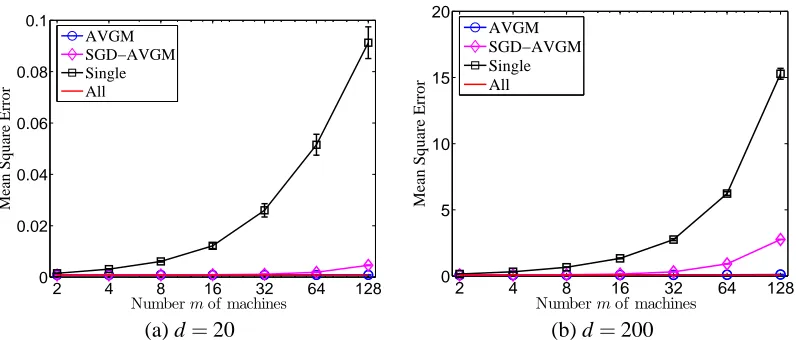
(a) d=20 (b) d=200
Figure 1: The errorkbθ−θ∗k22versus number of machines, with standard errors across twenty simu-lations, for solving least squares with data generated according to the normal model (16). The oracle least-squares estimate using all N samples is given by the line “All,” while the line “Single” gives the performance of the naive estimator using only n=N/m samples.
(i) The AVGMmethod
(ii) The SAVGMmethod with several settings of the subsampling ratio r
(iii) The SGDAVGMmethod with stepsizeηt=d/(10(d+t)), which gave good performance. In addition to (i)–(iii), we also estimateθ∗with
(iv) The empirical minimizer of a single split of the data of size n=N/m (v) The empirical minimizer on the full data set (the oracle solution).
4.1 Averaging Methods
For our first set of experiments, we study the performance of the averaging methods (AVGMand SAVGM), showing their scaling as the number of splits of data—the number of machines m—grows for fixed N and dimensions d =20 and d=200. We use the standard regression model (16) to generate the data, and throughout we letbθdenote the estimate returned by the method under consid-eration (so in the AVGMcase, for example, this is the vectorbθ:=θ1). The data samples consist of pairs(x,y), where x∈Rdand y∈Ris the target value. To sample each x vector, we choose five dis-tinct indices in{1, . . . ,d}uniformly at random, and the entries of x at those indices are distributed as N(0,1). For the model (16), the population optimal vectorθ∗is u.
In Figure 1, we plot the errorkbθ−θ∗k22of the inferred parameter vectorbθfor the true parameters
θ∗versus the number of splits m, or equivalently, the number of separate machines available for use.
We also plot standard errors (across twenty experiments) for each curve. As a baseline in each plot, we plot as a red line the squared errorkbθN−θ∗k22of the centralized “gold standard,” obtained by applying a batch method to all N samples.
2 4 8 16 32 64 128 10−7
10−6 10−5 10−4 10−3 10−2
Numbermof machines
Mean Square Error
AVGM−All SGD-AVGM−All
2 4 8 16 32 64 128
10−4 10−3 10−2 10−1 100 101
Numbermof machines
Mean Square Error
AVGM−All SGD-AVGM−All
(a) d=20 (b) d=200
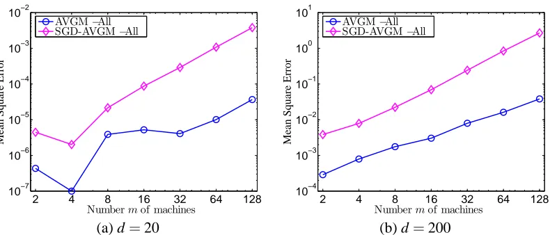
Figure 2: Comparison of AVGM and SGDAVGM methods as in Figure 1 plotted on logarithmic
scale. The plot showskbθ−θ∗k22− kθN−θ∗k22, whereθNis the oracle least-squares esti-mator using all N data samples.
solution using only a fraction 1/m of the data. In particular, ifbθis obtained by the batch method, then AVGMis almost as good as the full-batch baseline even for m as large as 128, though there is some evident degradation in solution quality. The SGDAVGM (stochastic-gradient with averaging) solution also yields much higher accuracy than the naive solution, but its performance degrades more quickly than the AVGM method’s as m grows. In higher dimensions, both the AVGM and SGDAVGM procedures have somewhat worse performance; again, this is not unexpected since in high dimensions the strong convexity condition is satisfied with lower probability in local data sets. We present a comparison between the AVGMmethod and the SGDAVGM method with some-what more distinguishing power in Figure 2. For these plots, we compute the gap between the AVGMmean-squared-error and the unparallel baseline MSE, which is the accuracy lost due to par-allelization or distributing the inference procedure across multiple machines. Figure 2 shows that the mean-squared error grows polynomially with the number of machines m, which is consistent with our theoretical results. From Corollary 3, we expect the AVGMmethod to suffer (lower-order) penalties proportional to m2 as m grows, while Theorem 5 suggests the somewhat faster growth we see for the SGDAVGM method in Figure 2. Thus, we see that the improved run-time perfor-mance of the SGDAVGMmethod—requiring only a single pass through the data on each machine, touching each datum only once—comes at the expense of some loss of accuracy, as measured by mean-squared error.
4.2 Subsampling Correction
We now turn to developing an understanding of the SAVGMalgorithm in comparison to the standard
2 4 8 16 32 64 128 0.7
0.8 0.9 1 1.1 1.2 1.3x 10
−3
Numbermof machines
Mean Square Error
AVGM
SAVGM (r=0.005) SAVGM (r=0.01) SAVGM (r=0.02) All
2 4 8 16 32 64 128
0.05 0.1 0.15 0.2 0.25
Numbermof machines
Mean Square Error
AVGM SAVGM (r=0.01) SAVGM (r=0.02) SAVGM (r=0.04) All
(a) d=20 (b) d=200
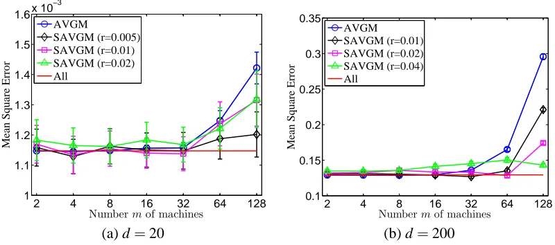
Figure 3: The errorkbθ−θ∗k22plotted against the number of machines m for the AVGMand SAVGM
methods, with standard errors across twenty simulations, using the normal regression model (16). The oracle estimator is denoted by the line “All.”
2 4 8 16 32 64 128
1 1.1 1.2 1.3 1.4 1.5 1.6x 10
−3
Numbermof machines
Mean Square Error
AVGM
SAVGM (r=0.005) SAVGM (r=0.01) SAVGM (r=0.02) All
2 4 8 16 32 64 128
0.1 0.15 0.2 0.25 0.3 0.35
Numbermof machines
Mean Square Error
AVGM SAVGM (r=0.01) SAVGM (r=0.02) SAVGM (r=0.04) All
(a) d=20 (b) d=200
Figure 4: The errorkbθ−θ∗k22plotted against the number of machines m for the AVGMand SAVGM
methods, with standard errors across twenty simulations, using the non-normal regression model (18). The oracle estimator is denoted by the line “All.”
we expect to see some performance gains. In our experiments, we use multiple sub-sampling rates to study their effects, choosing r∈ {0.005,0.01,0.02,0.04}, where we recall that the output of the SAVGMalgorithm is the vectorbθ:= (θ1−rθ2)/(1−r).
We begin with experiments in which the data is generated as in the previous section. That is, to generate a feature vector x∈d, choose five distinct indices in{1, . . . ,d}uniformly at random, and the entries of x at those indices are distributed as N(0,1). In Figure 3, we plot the results of simulations comparing AVGM and SAVGM with data generated from the normal regression model (16). Both
algorithms have have low error rates, but the AVGM method is slightly better than the SAVGM
1 2 4 8 16 32 64 128 256 512 10242048 4096 8192 0
0.002 0.004 0.006 0.008 0.01 0.012 0.014 0.016 0.018 0.02
Numb ermof machines
k
θ
−
θ
∗k 2 2
AVGM
SAVGM(r= (d/n)2/3)
1 2 4 8 16 32 64 128 256 512 1024 2048 40968192 0
0.005 0.01 0.015 0.02 0.025 0.03 0.035 0.04
Numb er mof machines
k
θ
−
θ
∗k 2 2
AVGM
SAVGM(r= (d/n)2/3)
(a) d=20 (b) d=40
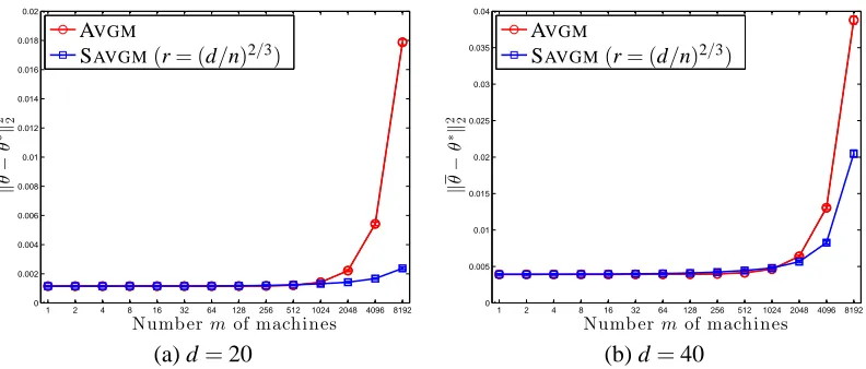
Figure 5: The errorkbθ−θ∗k22plotted against the number of machines m for the AVGMand SAVGM
methods using regression model (17).
case the SAVGMmethod does not offer improvement over AVGM, since the estimators are unbiased. (In Figure 3(a), we note that the standard error is in fact very small, since the mean-squared error is only of order 10−3.)
To understand settings in which subsampling for bias correction helps, in Figure 4, we plot mean-square error curves for the least-squares regression problem when the vector y is sampled according to the non-normal regression model (18). In this case, the least-squares estimator is biased forθ∗(which, as before, we estimate by solving a larger regression problem using 10N data samples). Figure 4 shows that both the AVGMand SAVGM method still enjoy good performance; in some cases, the SAVGM method even beats the oracle least-squares estimator for θ∗ that uses all N samples. Since the AVGM estimate is biased in this case, its error curve increases roughly quadratically with m, which agrees with our theoretical predictions in Theorem 1. In contrast, we see that the SAVGMalgorithm enjoys somewhat more stable performance, with increasing benefit as the number of machines m increases. For example, in case of d=200, if we choose r=0.01 for m≤32, choose r=0.02 for m=64 and r=0.04 for m=128, then SAVGM has performance comparable with the oracle method that uses all N samples. Moreover, we see that all the values of r—at least for the reasonably small values we use in the experiment—provide performance improvements over a non-subsampled distributed estimator.
For our final simulation, we plot results comparing SAVGMwith AVGMin model (17), which is mis-specified but still a normal model. We use a simpler data generating mechanism, specifically, we draw x∼N(0,Id×d)from a standard d-dimensional normal, and v is chosen uniformly in[0,1];
in this case, the population minimizer has the closed formθ∗=u+3v. Figure 5 shows the results for dimensions d =20 and d=40 performed over 100 experiments (the standard errors are too small to see). Since the model (17) is not that badly mis-specified, the performance of the SAVGM
Feature Name Dimension Description
Query 20000 Word tokens appearing in the query. Gender 3 Gender of the user
Keyword 20000 Word tokens appearing in the purchase keywords. Title 20000 Word tokens appearing in the ad title.
Advertiser 39191 Advertiser’s ID AdID 641707 Advertisement’s ID. Age 6 Age of the user
UserFreq 25 Number of appearances of the same user. Position 3 Position of advertisement on search page. Depth 3 Number of ads in the session.
QueryFreq 25 Number of occurrences of the same query. AdFreq 25 Number of occurrences of the same ad. QueryLength 20 Number of words in the query.
TitleLength 30 Number of words in the ad title. DespLength 50 Number of words in the ad description. QueryCtr 150 Average click-through-rate for query. UserCtr 150 Average click-through-rate for user. AdvrCtr 150 Average click-through-rate for advertiser.
WordCtr 150 Average click-through-rate for keyword advertised. UserAdFreq 20 Number of times this user sees an ad.
UserQueryFreq 20 Number of times this user performs a search.
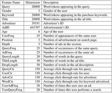
Table 1: Features used in online advertisement prediction problem.
5. Experiments with Advertising Data
Predicting whether a user of a search engine will click on an advertisement presented to him or her is of central importance to the business of several internet companies, and in this section, we present experiments studying the performance of the AVGMand SAVGMmethods for this task. We use a large data set from the Tencent search engine,soso.com(Sun, 2012), which contains 641,707 distinct advertisement items with N=235,582,879 data samples.
Each sample consists of a so-called impression, which in the terminology of the information retrieval literature (e.g., see the book by Manning et al., 2008), is a list containing a user-issued search, the advertisement presented to the user in response to the search, and a label y∈ {+1,−1} indicating whether the user clicked on the advertisement. The ads in our data set were presented to 23,669,283 distinct users.
8 16 32 64 128 0.1295
0.13 0.1305 0.131 0.1315 0.132
Number of machinesm
Negative Log−Likelihood
SAVGM (r=0.1) SAVGM (r=0.25)
AVGM
1 2 3 4 5 6 7 8 9 10
0.1295 0.13 0.1305 0.131 0.1315 0.132
Negative Log−Likelihood
Number of Passes
SDCA SGD
(a) (b)
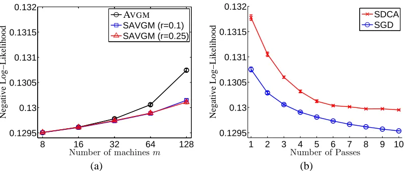
Figure 6: The negative log-likelihood of the output of the AVGM, SAVGM, and stochastic methods on the held-out data set for the click-through prediction task. (a) Performance of the AVGMand SAVGM methods versus the number of splits m of the data. (b) Performance of SDCA and SGD baselines as a function of number of passes through the entire data set.
each of which is assigned an index in x. (Note that the intervals and number thereof vary per feature, and the dimension of the features listed in Table 1 corresponds to the number of intervals). When a feature falls into a particular bin, the corresponding entry of x is assigned a 1, and otherwise the en-tries of x corresponding to the feature are 0. Each feature has one additional value for “unknown.” The remaining categorical features—gender, advertiser, and advertisement ID (AdID)—are also given{0,1}encodings, where only one index of x corresponding to the feature may be non-zero (which indicates the particular gender, advertiser, or AdID). This combination of encodings yields a binary-valued covariate vector x∈ {0,1}d with d=741,725 dimensions. Note also that the fea-tures incorporate information about the user, advertisement, and query issued, encoding information about their interactions into the model.
Our goal is to predict the probability of a user clicking a given advertisement as a function of the covariates in Table 1. To do so, we use a logistic regression model to estimate the probability of a click response
P(y=1|x;θ):= 1
1+exp(−hθ,xi),
whereθ∈Rd is the unknown regression vector. We use the negative logarithm of P as the loss, incorporating a ridge regularization penalty. This combination yields instantaneous loss
f(θ;(x,y)) =log(1+exp(−yhθ,xi)) +λ
2kθk 2 2.
In all our experiments, we assume that the population negative log-likelihood risk has local strong convexity as suggested by Assumption 2. In practice, we use a small regularization parameter
λ=10−6to ensure fast convergence for the local sub-problems.
log-loss on a held-out data set. Specifically, we perform a five-fold validation experiment, where we shuffle the data and partition it into five equal-sized subsets. For each of our five experiments, we hold out one partition to use as the test set, using the remaining data as the training set for inference. When studying the AVGM or SAVGM method, we compute the local estimateθi via a trust-region Newton-based method (Nocedal and Wright, 2006) implemented by LIBSVM (Chang and Lin, 2011).
The data set is too large to fit in the memory of most computers: in total, four splits of the data require 55 gigabytes. Consequently, it is difficult to provide an oracle training comparison using the full N samples. Instead, for each experiment, we perform 10 passes of stochastic dual coordinate ascent (SDCA) (Shalev-Shwartz and Zhang, 2012) and 10 passes of stochastic gradient descent (SGD) through the data set to get two rough baselines of the performance attained by the empirical minimizer for the entire training data set. Figure 6(b) shows the hold-out set log-loss after each of the sequential passes through the training data finishes. Note that although the SDCA enjoys faster convergence rate on the regularized empirical risk (Shalev-Shwartz and Zhang, 2012), the plot shows that the SGD has better generalization performance.
In Figure 6(a), we show the average hold-out set log-loss (with standard errors) of the estimator
θ1provided by the AVGMmethod versus number of splits of the data m, and we also plot the log-loss of the SAVGM method using subsampling ratios of r∈ {.1, .25}. The plot shows that for small m,
both AVGMand SAVGMenjoy good performance, comparable to or better than (our proxy for) the oracle solution using all N samples. As the number of machines m grows, however, the de-biasing provided by the subsampled bootstrap method yields substantial improvements over the standard AVGM method. In addition, even with m=128 splits of the data set, the SAVGM method gives better hold-out set performance than performing two passes of stochastic gradient on the entire data set of m samples; with m=64, SAVGMenjoys performance as strong as looping through the data four times with stochastic gradient descent. This is striking, since doing even one pass through the data with stochastic gradient descent gives minimax optimal convergence rates (Polyak and Juditsky, 1992; Agarwal et al., 2012). In ranking applications, rather than measuring negative log-likelihood, one may wish to use a direct measure of prediction error; to that end, Figure 7 shows plots of the area-under-the-curve (AUC) measure for the AVGM and SAVGM methods; AUC is a well-known measure of prediction error for bipartite ranking (Manning et al., 2008). Broadly, this plot shows a similar story to that in Figure 6.
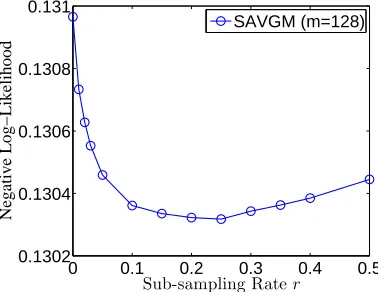
It is instructive and important to understand the sensitivity of the SAVGM method to the value of the resampling parameter r. We explore this question in Figure 8 using m=128 splits, where we plot the log-loss of the SAVGMestimator on the held-out data set versus the subsampling ratio r. We choose m=128 because more data splits provide more variable performance in r. For the
soso.comad prediction data set, the choice r=.25 achieves the best performance, but Figure 8
suggests that mis-specifying the ratio is not terribly detrimental. Indeed, while the performance of SAVGM degrades to that of the AVGM method, a wide range of settings of r give improved performance, and there does not appear to be a phase transition to poor performance.
6. Discussion
meth-8 16 32 64 128 0.784
0.785 0.786 0.787 0.788 0.789 0.79 0.791
Number of machinesm
Area under ROC curve
SAVGM (r=0.1) SAVGM (r=0.25)
AVGM
Figure 7: The area-under-the-curve (AUC) measure of ranking error for the output of the AVGM
and SAVGMmethods for the click-through prediction task.
0 0.1 0.2 0.3 0.4 0.5 0.1302
0.1304 0.1306 0.1308 0.131
Negative Log−Likelihood
Sub-sampling Rater
SAVGM (m=128)
Figure 8: The log-loss on held-out data for the SAVGMmethod applied with m=128 parallel splits of the data, plotted versus the sub-sampling rate r.
Acknowledgments
We thank Joel Tropp for some informative discussions on and references for matrix concentration and moment inequalities. We also thank Ohad Shamir for pointing out a mistake in the statements of results related to Theorem 1, and the editor and reviewers for their helpful comments and feedback. JCD was supported by the Department of Defence under the NDSEG Fellowship Program and by a Facebook PhD fellowship. This work was partially funded by Office of Naval Research MURI grant N00014-11-1-0688 to MJW.
Appendix A. The Necessity of Smoothness
Here we show that some version of the smoothness conditions presented in Assumption 3 are nec-essary for averaging methods to attain better mean-squared error than using only the n samples on a single processor. Given the loss function (5), let n0=∑ni=11(Xi=0)to be the count of 0 samples.
Usingθ1as shorthand forθ1,i, we see by inspection that the empirical minimizerθ1is
θ1=
(n 0
n −
1
2 when n0≤n/2 1−2nn
0 otherwise.
For simplicity, we may assume that n is odd. In this case, we obtain that
E[θ1] = 1 4+E
hn0
n1(n0<n/2) i
−E
n 2n0
1(n0>n/2)
=1
4+ 1 2n
⌊n/2⌋
∑
i=0
n i i n− 1 2n n
∑
i=⌈n/2⌉ n i n 2i= 1 4+ 1 2n
⌊n/2⌋
∑
i=0
n i i n− n 2(n−i)
by the symmetry of the binomial. Adding and subtracting12 from the term within the braces, noting that P(n0<n/2) =1/2, we have the equality
E[θ1] = 1 2n
⌊n/2⌋
∑
i=0
n i i n− n 2(n−i)+
1 2
= 1
2n ⌊n/2⌋
∑
i=0
n i
i(n−2i)
2n(n−i).
If Z is distributed normally with mean 1/2 and variance 1/(4n), then an asymptotic expansion of the binomial distribution yields
1 2
n⌊n/2⌋
∑
i=0
n i
i(n−2i)
2n(n−i) =E
Z(1−2Z)
2−2Z |0≤Z≤ 1 2
+o(n−1/2)
≥12E
Z−2Z2|0≤Z≤1 2
+o(n−1/2) =Ω(n−12),
Appendix B. Proof of Theorem 1
Although Theorem 1 is in terms of bounds on 8th order moments, we prove a somewhat more general result in terms of a set of(k0,k1,k2)moment conditions given by
E[k∇f(θ; X)kk0
2]≤Gk0, E[
∇2f(θ; X)−∇2F 0(θ)
k1
2]≤H
k1,
E[L(X)k2]≤Lk2 and E[(L(X)−E[L(X)])k2]≤Lk2
forθ∈U . (Recall the definition of U prior to Assumption 3). Doing so allows sharper control if higher moment bounds are available. The reader should recall throughout our arguments that we have assumed min{k0,k1,k2} ≥8. Throughout the proof, we use F1 andθ1 to indicate the local empirical objective and empirical minimizer of machine 1 (which have the same distribution as those of the other processors), and we recall the notation 1(E)for the indicator function of the event
E
.Before beginning the proof of Theorem 1 proper, we begin with a simple inequality that relates the error term θ−θ∗ to an average of the errors θi−θ∗, each of which we can bound in turn. Specifically, a bit of algebra gives us that
E[θ−θ∗2 2] =E
1 m
m
∑
i=1
θi−θ∗
2 2
= 1
m2
m
∑
i=1
E[kθi−θ∗k2 2] +
1 m2
∑
i6=j
E[θi−θ∗,θj−θ∗]
≤m1E[kθ1−θ∗k22] +m(m−1)
m2 kE[θ1−θ∗]k 2 2
≤m1E[kθ1−θ∗k2
2] +kE[θ1−θ∗]k22. (19) Here we used the definition of the averaged vectorθand the fact that for i6= j, the vectorsθiandθj
are statistically independent, they are functions of independent samples. The upper bound (19) illu-minates the path for the remainder of our proof: we bound each ofE[kθi−θ∗k2
2]andkE[θi−θ∗]k 2 2. Intuitively, since our objective is locally strongly convex by Assumption 2, the empirical minimiz-ing vectorθ1is a nearly unbiased estimator forθ∗, which allows us to prove the convergence rates in the theorem.
We begin by defining three events—which we (later) show hold with high probability—that guarantee the closeness of θ1 and θ∗. In rough terms, when these events hold, the function F1 behaves similarly to the population risk F0around the pointθ∗; since F0is locally strongly convex, the minimizerθ1of F1will be close toθ∗. Recall that Assumption 3 guarantees the existence of a ball Uρ={θ∈Rd:kθ−θ∗k
2<ρ}of radiusρ∈(0,1)such that
∇2f(θ; x)
−∇2f(θ′; x)2≤L(x)θ−θ′2
for all θ,θ′ ∈Uρ and any x, where E[L(X)k2]≤Lk2. In addition, Assumption 2 guarantees that
∇2F