Efficient Computation of Gaussian Process Regression for
Large Spatial Data Sets by Patching Local Gaussian
Processes
Chiwoo Park [email protected]
Department of Industrial and Manufacturing Engineering Florida State University
2525 Pottsdamer St., Tallahassee, FL 32310-6046, USA
Jianhua Z. Huang [email protected]
Department of Statistics Texas A&M University
3143 TAMU, College Station, TX 77843-3143, USA
Editor:Manfred Opper
Abstract
This paper develops an efficient computational method for solving a Gaussian process (GP) regression for large spatial data sets using a collection of suitably defined local GP regressions. The conventional local GP approach first partitions a domain into multiple non-overlapping local regions, and then fits an independent GP regression for each local region using the training data belonging to the region. Two key issues with the local GP are (1) the prediction around the boundary of a local region is not as accurate as the prediction at interior of the local region, and (2) two local GP regressions for two neighboring local regions produce different predictions at the boundary of the two regions, creating undesirable discontinuity in the prediction. We address these issues by constraining the predictions of local GP regressions sharing a common boundary to satisfy the same boundary constraints, which in turn are estimated by the data. The boundary constrained local GP regressions are solved by a finite element method. Our approach shows competitive performance when compared with several state-of-the-art methods using two synthetic data sets and three real data sets.
Keywords: constrained Gaussian process regression, kriging, local regression, boundary value problem, spatial prediction, variational problem
1. Introduction
Within its origin in geostatistics and known as kriging, the Gaussian process regression (hereafter abbreviated as GP regression) has been developed to be a useful tool in machine learning (Rasmussen and Williams, 2005). It provides the best linear unbiased prediction computable by a simple closed-form expression, which also has a nice probabilistic interpre-tation (MacKay, 1998). However, computing the exact solution of a GP regression requires
high for data sets of large size. The purpose of this paper is to develop a new computational method to expedite the computation of GP regression for large data sets.
The computation issue for GP regression has received much attention in machine learn-ing and spatial statistics. Since a major computation bottleneck for a GP regression is the inversion of a big sample covariance matrix of size N ×N, many approaches proposed to approximate the sample covariance matrix with a more easily invertible one. Covariance tapering (Furrer et al., 2006; Kaufman et al., 2008) tapers the original covariance function to make a sample covariance matrix sparser and applies the sparse matrix computation algorithms for faster inversion of the matrix. Low-rank approximation (Seeger et al., 2003; Snelson and Ghahramani, 2006; Cressie and Johannesson, 2008; Banerjee et al., 2008; Sang and Huang, 2012) introducesM latent variables and assumes a certain conditional indepen-dence given the latent variables, which reduces the rank of the resulting sample covariance matrix to M. The approximation of a Gaussian random field by a Gaussian Markov ran-dom field has also been proposed (Lindgren et al., 2011). When a covariance matrix of the approximated Gaussian random field is a Mat´ern covariance function, the sparse pre-cision matrix for the Gaussian Markov random field can be explicitly constructed, and the approximation can be efficiently computed.
On the other hand, local GP regression partitions a regression domain into local regions, and an independent GP regression model is learned for each local region. Since the number of observations belonging to a local region is much smaller than the total number of ob-servations, the resulting sample covariance matrix for a local GP regression becomes much smaller. However, because of the independence of the local GP regressions, two local GP regressions for two neighboring local regions produce different predictions at the boundary of the two regions. This discontinuity in prediction is not acceptable in applications. Many proposed methods have combined local GP regressions into a global model. A popular ap-proach is to take a mixture of local GP regressions through a Dirichlet mixture (Rasmussen and Ghahramani, 2002), a treed mixture (Gramacy and Lee, 2008), Bayesian model aver-aging (Tresp, 2000; Chen and Ren, 2009; Deisenroth and Ng, 2015), or a locally weighted projection (Nguyen-Tuong et al., 2009). Another approach is to use multiple additive co-variance functions of a global coco-variance and a local coco-variance (Snelson and Ghahramani, 2007; Vanhatalo and Vehtari, 2008), to simply construct a new local model for each testing location (Gramacy and Apley, 2015).
constrained local GP regressions using the finite element method. This is mathematically more elegant and conceptually simpler than the previously somewhat ad hoc treatment. In addition, we significantly improve the DDM by proposing two approaches for estimating the boundary constraints (i.e., boundary values of local regions). The improved accuracy of estimating these constraints leads to better prediction accuracy of our constrained local GP regressions. Last, our new approach has better numerical stability than the DDM. It was previously reported that the predictive variance estimate of the DDM can be negative for some numerical examples (Pourhabib et al., 2014). Since the expression of the DDM’s predictive variance estimate cannot be theoretically negative, the negative estimate is due to numerical issues. Our new approach provides positive predictive variances for all the ex-amples. The computation speed of the new approach is comparable to the DDM. When the domain in Rd is partitioned intoS local regions and each local region hasNS training data points, the computational cost of the proposed method is O(N NS2+dS), where NS N. Since our method can be viewed as “patching” a collection of local GP regressions, we refer to our method as patched Gaussian Process regression orpatched GP for short.
The proposed patched GP method is theoretically applicable for an arbitrary input dimensiond, but the implementation of the approach may be practically difficult ford >2 mainly due to hardness in generating finite element meshes for high dimensions. Therefore, the practical application of the proposed approach would be a GP regression with a spatial data set of large volume (i.e., the data fall in a domain inR2), which finds broad applications
in spatial statistics and remote sensing (Stein, 2012; Curran and Atkinson, 1998). We will still describe and derive our approach for a general dimension to ease a possible future extension of the approach to high dimensional problems. As a byproduct of this work, we develop a finite element method for the boundary constrained GP regression problem, which may have potential applications in GP solutions for partial differential equations (Graepel, 2003) or for linear stochastic differential equations having boundary conditions (Steinke and Sch¨olkopf, 2008).
2. Reformulation of Gaussian Process Regression as An Optimization Problem
A GP regression is formulated as follows: given a training setD={(xn, yn), n= 1, . . . , N} of N pairs of inputs xn and noisy outputs yn of a latent function f, obtain the predictive distribution of f at a test location x∗, denoted by f∗ =f(x∗). We assume that the latent function comes from a zero-mean Gaussian process with a covariance function k(·,·) and the noisy observations yi are given by
yi =f(xi) +i, i= 1, . . . , N,
where i ∼ N(0, σ2) are white noises independent of f(xi). Denote x = [x1, x2, . . . , xN]0 and y= [y1, y2, . . . , yN]0. The joint distribution of (f∗,y) is
P(f∗,y) =N
0,
k∗∗ k0x∗ kx∗ σ2I+Kxx
,
wherek∗∗=k(x∗, x∗),kx∗ = (k(x1, x∗), . . . , k(xN, x∗))0 and Kxx is an N×N matrix with
(i, j)th entity k(xi, xj). The subscripts ofk∗∗,kx∗, and Kxx represent two sets of locations between which the covariance is computed, and x∗ is abbreviated as ∗. The predictive distribution of f∗ given y is
P(f∗|y) =N(k0x∗(σ2I+Kxx)−1y, k∗∗−k0x∗(σ2I+Kxx)−1kx∗). (1)
The predictive mean k0x∗(σ2I +Kxx)−1y gives the point prediction of f(x) at location x∗, whose uncertainty is measured by the predictive variance k∗∗−k0x∗(σ2I+Kxx)−1kx∗.
Efficient calculation of the predictive mean and variance has been the focus of much research. The predictive mean and variance can be derived using the viewpoint of the best linear unbiased predictor (BLUP) as follows. Consider all linear predictors
µ(x∗) =u(x∗)0y, (2)
which automatically satisfy the unbiasedness requirement E[µ(x∗)] = 0 since all random variables yi have zero mean. We seek anN-dimensional vector u(x∗) such that the mean squared prediction errorE[µ(x∗)−f(x∗)]2 is minimized. SinceE[µ(x∗)] = 0 andE[f(x∗)] = 0, the mean squared prediction error equals the error variance var[µ(x∗)−f(x∗)] and can be expressed as
σ(x∗) =u(x∗)0E(yy0)u(x∗)−2u(x∗)0E(yf∗) +E(f∗2)
=u(x∗)0(σ2I+Kxx)u(x∗)−2u(x∗)0kx∗+k∗∗, (3)
which is a quadratic form inu(x∗). It is easy to seeσ(x∗) is minimized if and only ifu(x∗) is chosen to be (σ2I+K
xx)−1kx∗; moreover, the minimal value ofσ(x∗) equals the predictive
variance given in (1).
The BLUP view of GP regression suggests a reformulation of GP regression as the following optimization problem:
Minimize u(x∗)∈RN
z[u(x∗)] = 1 2u(x∗)
where A = (σ2I +Kxx) is an N ×N positive definite matrix, and f(x∗) = kx∗ is a N ×1 vectorial function. Note that the objective function in (4) equals half of the error variance of a linear predictor given in (3) subtracting the constant term k∗∗/2. The one half factor is introduced here to make subsequent formulas neat. The solution of (4) is
u†(x∗) =A−1kx∗= (σ2I+Kxx)−1kx∗. Back to the GP regression problem, the predictive mean is given byu†(x∗)tyand the predictive variance is 2z[u†(x∗)] +k∗∗, twice the optimal objective value plus the variance off∗ at the locationx∗.
Usually we are interested in obtaining the predictive mean and variance at multiple locations in a domain Ω⊂RN, where all training locationsx
i’s also belong to. To consider the prediction at all locations in Ω, we consider the following optimization problem:
Minimize
u(·)∈[L2(Ω)]N J(u) =
Z
Ω
1 2u(x)
0Au(x)−f(x)0u(x)
dx, (5)
where [L2(Ω)]N is the Cartesian product ofN Hilbert spacesL2(Ω). The objective function
here is simply the integration of the objective function in the single location problem (4). Since the optimal solution u†(x∗) obtains the minimum objective value of (4) at every locationx∗∈Ω, u†(x∗) as a function ofx∗ also solves the global problem (5).
According to a standard result from functional analysis (Ern and Guermond, 2004), the problem (5) has an equivalent variational formulation, as follows.
Proposition 1 The vectoru∈[L2(Ω)]N minimizesJ(u)if and only if it solves the integral equation
Z
Ω
u(x)0Av(x)dx= Z
Ω
f(x)0v(x)dx for each v∈[L2(Ω)]N. (6) The proof is given in Appendix A.
Throughout the rest of the paper, whenever no confusion may arise and to alleviate the notation, we omit the Lebesgue measure under the integral sign. For example, we shall write RΩu0Av and RΩf0v instead ofRΩu(x)0Av(x)dxand RΩf(x)0v(x)dx.
3. Gaussian Process Regression with Boundary Constraints
The optimization problem (5) was introduced in previous section as a reformulation of the GP regression. Now we introduce boundary constraints to the GP regression through this optimization problem and develop a finite element solution for the corresponding variational formulation. This finite element solution will serve as a building block in the next section for the patched GP regression, which consists of a collection of boundary constrained GP regressions.
3.1 Constrained Optimization Problem and Its Variational Formulation
We require that the domain Ω is a Lipschitz bounded open set. Let∂Ω denote the boundary of the domain Ω. We need to restrict our attention to smooth functions and specifically consider only solution vectors in the Sobolev space [H1(Ω)]N instead of [L2(Ω)]N, where
the value of a function in this space can be unbounded on ∂Ω and so not well-defined. For example, take Ω = (0,1) and u(x) = x−1/3. It is clear that u(x) ∈ L2(Ω) but u(0) = ∞. On the other hand, the values of a function inH1(Ω) are bounded at its domain boundary. In fact, if u ∈ H1(Ω), then u restricted on ∂Ω, which we denote by u|∂Ω, is a member of H1/2(∂Ω) :={u∈L2(Ω) : ||xu−(xy)−||(du+1)(y)/2 ∈L
2(Ω×Ω)} (Ern and Guermond, 2004, Theorem
B.52).
Consider the boundary constraints of the form y0u(x) =b(x) for some known function
b ∈ H1/2(∂Ω). Since y0u(x) can be interpreted as a linear predictor at location x, the constrains simply require the predictions at the domain boundary to have certain specified functional form. Denote
Hb =
u∈[H1(Ω)]N : Z
∂Ω
y0u|∂Ωv=
Z
∂Ω
b v for each v∈H1/2(∂Ω)
.
A constrained version of the optimization problem (5) can be written as
Minimize u∈Hb
J(u) = Z
Ω
1 2u(x)
0Au(x)−f(x)0u(x)
dx. (7)
Here, for mathematical convenience, we have replaced the strict boundary constraints y0u(x) =b(x) by a weaker form foru∈Hb.
Similar to Proposition 1, we can show that the optimization problem (7) is equivalent to a variational formulation:
Proposition 2 The vector u ∈ Hb minimizes J(u) if and only if it solves the integral
equation
Z
Ω
u(x)0Av(x)dx= Z
Ω
f(x)0v(x)dx for each v∈Hb. (8)
The proof is given in Appendix B.
3.2 Finite Element Approximation
A finite element method approximates the spaceHbof vector-valued functions on a domain Ω by a finite dimensional vector space. With the approximation, the integral equation (8) is converted to a finite-dimensional linear system of equations.
For any vector-valued function u ∈ [H1(Ω)]N, let u|Km denote its restriction to Km,
i.e., u(x)|Km = 1Km(x)u(x). The finite element approximation ofu on Km is given by
u|Km ≈umh:=
p X
j=1
βmjφmj,
whereβmj is anN-vector of coefficients in the basis expansion. The combination of umh’s overKm,m∈M, provides a global approximation ofu over the whole domain Ω, i.e.,
uh = M X
m=1
umh= M X
m=1
p X
j=1
βmjφmj, (9)
which has a matrix-vector representation
uh =U0φ, (10)
whereU is the (M p)×N matrix formed by concatenating row vectorsβ0mj in row-wise and
φis the (M p)-dimensional column vector of φmj’s. In (9) and (10) we explicitly extended
φmj to be zero outside Km. The collection of vector-valued functions with expression (10) is a finite-dimensional linear space. We call this space the finite element space and denote it asGh, where the subscript denotes the mesh sizeh.
The finite element method for solving the unconstrained integral equation (6) seeks
uh ∈Gh such that
a(uh,vh) =c(vh) for each vh∈Gh, (11)
where a(u,v) = Ru0Av and c(v) = R f0v. Following (10), we can write uh = U0φ and similarlyvh=V0φ. Both of the lhs and rhs of (11) can be simply represented as algebraic forms as follows. First, since
u0hAvh = trace(φ0U AV0φ) = trace(φφ0U AV0),
we have
a(uh,vh) = Z
Ω
u0hAvh = trace( Z
Ω
φφ0U AV0) = trace(ΦU AV0),
whereΦ=R
Ωφφ
0. Second, since
f0vh= trace(f0V0φ) = trace(φf0V0),
we have that
c(vh) = Z
Ω
f0vh = trace( Z
Ω
φf0V0) = trace(F V0),
whereF =RΩφf0. Therefore, the integral equation (11) is equivalent to the following linear system
trace((ΦU A−F)V0) = 0 for each V ∈RN×(M p),
which is equivalent to
We now introduce the boundary constraints. We partition (after reordering the el-ements) the basis function vector φ used in uh = U0φ into two vectors φ0 and φb in column-wise such that, φ0 is a column vector of the φmj(x)’s satisfyingφmj|∂Ω = 0 andφb is a column vector of theφmj(x)’s satisfying φmj|∂Ω 6= 0. Suppose that φ0 hasQ elements
and φb hasR elements. Since the number of columns ofφis M p,Q+R =M p. With the partition, we have that
uh =U00φ0+U0bφb, (13) where U0 and Ub are submatrices consisting of U’s rows corresponding to φ0 and φb respectively. Substituting (13) into equation (12), we have that
Φ0U0+ΦbUb =F A−1, (14)
whereΦ0 =
R
Ωφφ 0
0 and Φb = R
Ωφφ 0
b.
The boundary constraints restricted to Gh can be written as Z
∂Ω
y0uh|∂Ωv=
Z
∂Ω
b v for each v∈Gh.
Using (14) and dropping the basis functions whose values are zero at the boundary, we obtain
Z
∂Ω
y0U0bφb|∂Ωφmj|∂Ω=
Z
∂Ω
b φmj|∂Ω for each φmj|∂Ω6= 0,
which implies
Z
∂Ω
y0U0bφb|∂Ωφ0b|∂Ω= Z
∂Ω
bφ0b|∂Ω.
Letting B=R
∂Ωφb|∂Ωφ0b|∂Ω and b=
R ∂Ωbφ
0
b|∂Ω, we have
y0U0bB=b0, (15)
We decompose Ub into two components: one orthogonal toy and the residual. LetOy beN×(N−1) matrix ofN−1 column vectors orthogonal to y, which can be obtained by the Gram-Schmidt process. There existZ ∈RR×(N−1) and z∈
RR×1 satisfying
Ub=ZO0y+zy0. (16)
Therefore, (14) becomes
Φ0U0+ΦbZOy0 +Φbzy0 =F A−1 (17) Since
y0U0b =y0(OyZ0+yz0) =y0yz0,
equation (15) gives us
y0yz0B =b0,
therefore,
(y0y)z =B−1b. (18)
In summary, we first solve (18) forz, then solve (17) for U0 and Z, and then calculate Ub using (16). The finite element solution of the variational problem (8) is given byuh =
U0φ0+Ubφb. By the theory of finite element method (Ern and Guermond, 2004), the approximate solutionuh converges to the solution of the original problem as the mesh size
4. Patching Constrained Local GPs for Efficient Computation of Global GP regression
This section presents our patched GP regression method. We start from some notations. We partition the domain Ω of the data into small local regions {Ωs, s = 1, . . . , S} and partition the training data set D= {(xn, yn) :n = 1, . . . , N} accordingly into S data sets
Ds:= {(xn, yn)∈ D:xn∈Ωs}. We then calculate the local prediction function fs for the local region Ωs using the data set Ds. There are some issues with this localized solution. First, the prediction at around ∂Ωs is not as accurate as the prediction at the interior of Ωs mainly because of the less number of observations available around ∂Ωs. In particular, when S becomes large, the boundary regions also increase. Therefore, the inaccuracy at the boundaries∂Ωs can have significant negative effects on the overall prediction accuracy. Second, two local GP regressions from two neighboring local regions Ωs and Ωt produce different predictionsfsand ftat the shared boundary, making the prediction discontinuous on the boundary. This discontinuity is unacceptable since continuity of the prediction is often desired. We propose to impose boundary constraints such that the two neighboring local GP regressions give the same predictions on the shared boundary.
Section 4.1 applies the finite element method of Section 3 to solve a boundary con-strained local GP problem for each local region when the boundary constraints are given. Section 4.2 gives two methods for estimating the boundary constraints. Section 4.3 dis-cusses some implementation details, including calculation of the integrations involving the finite elements, and learning parameters of the covariance function of the GP regression.
4.1 Boundary-constrained Local GP
For two neighboring local regions Ωsand Ωt, let Γst= Ωs∩Ωtdenote the shared boundary, where Ωs is the closure of Ωs. The prediction functionf specialized on Γst is denoted by a boundary function bst(x) forx ∈Γst. For the time being, we assume that bst(x) is known and shall discuss in next section how to estimate bst(x). Fix a domain Ωs, suppose all its boundary functions{bst :∀t,Γst6=∅}are known. Consider the following local GP problem on Ωs
Minimize us
J(us) = Z
Ωs
1 2us(x)
0A
sus(x)−fs(x)0us(x)
dx
subject toy0sus(x) =bst(x) onx∈Γst, ∀t, Γst 6=∅
(19)
whereAs,fs(x) andysare the localized versions ofA,f(x) andy, which are all computed using the data in Ωs. The constraints used in (19) restrict two local GP prediction functions
fs and ft to have the same predictionbst on the shared boundary Γst.
As in Section 3, we replace the boundary constraints by the weak form, approximate
us by its finite element approximationus,h=U0s,0φs,0+U0s,bφs,b, whereφs,0 is a vector of
local basis functions φmj’s satisfyingφmj(x)|Γst = 0 for all t’s, andφs,b is a vector of local
basis functions φmj’s satisfyingφmj(x)|Γst 6= 0 for all t’s, andφs = (φ
0
s,0,φ0s,b)0. Let Ns be the length of ys and Oys be Ns×(Ns−1) matrix of Ns−1 column vectors orthogonal to
ys. We can decompose Us,b into Us,b = ZsO0ys +zsy
0
system of equations forUs,0,Zs andzs,
Φs,0Us,0+Φs,bZsO0ys+Φs,bzsy0s=FsA−1s , (y0sys)zs=B−1s bs,
(20)
whereΦs,0 =
R
Ωsφsφ
0
s,0,Φs,b= R
Ωsφsφ
0
s,b,Fs= R
Ωsφsf
0
s, and
Bs= X
t:Γst6=∅
Z
Γst
φs,b|Γstφs,b|Γst,
bs= X
t:Γst6=∅
Z
Γst
bst|Γstφs,b|Γst.
Since bst(x) is unknown, we need to estimate bs using the procedure to be described in Section 4.2. Using the second equation of (20), we obtain zs =B−1s bs/y0sys. Substituting this expression ofzs in the first equation of (20), we obtain
Φs,0Us,0+Φs,bZsO0ys =FsA
−1
s −Φs,bzsy0s,
=FsA−1s −Φs,b
B−1s bsy0s
y0
sys
. (21)
We then solve this equation forUs,0andZs, and computeUs,b=ZsO0ys+zsy0s. Finally the finite element solution of the constrained local GP problem (19) isus,h=U0s,0φs,0+U
0
s,bφs,b. When the number of mesh cells in each local region is M on average and the number of training data in each domain is NS, the computation complexity of solving the constrained local GP regression (21) for one local region is O(NS3 +M2). The first part NS3 is for inverting Aj, and the second part is for inverting Φs,0 and Φs,b, which is proportional to
M2 because Φs,0 and Φs,b are sparse banded matrices; note that the complexity of solving a linear system with a banded coefficient matrix is proportional to the square of the size of the linear system (Mahmood et al., 1991). The cost per local region is mostly bounded by the cubic term O(NS3). The total computational cost for S local regions is thus O(SNS3), which also equals toO(N N2
S).
4.1.1 Illustrative Output of the Constrained GP Formulation
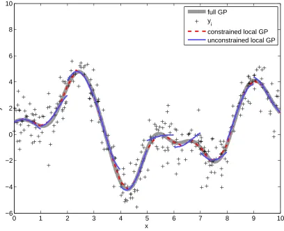
Our constrained local GP regression provides a good approximate to a full GP regression when the value of boundary function bst is close to the mean prediction of the full GP regression at Γ. To show this, we performed a simple simulation study. In the study, we generated a data set of 6,000 noisy observations from a zero-mean Gaussian process with an exponential covariance function,
yi =f(xi) +i fori= 1, . . . ,6000,
0 1 2 3 4 5 6 7 8 9 10 −6
−4 −2 0 2 4 6 8 10
x
y
full GP y
i
constrained local GP unconstrained local GP
Figure 1: Effect of the boundary constraint on Gaussian process regression.
and the 300 observations were distributed into the local regions accordingly. For each do-main, an unconstrained GP regression (unconstrained local GP) and a constrained GP re-gression (constrained local GP) were learned. When the constrained local GP was learned, the values of the regression outcome at the boundary points were constrained to be equal to the mean prediction of a full GP regression at the points. Note this is not a fair comparison since the full GP prediction was used. This example was just used to show the room for improvement if constraints are used.
4.2 Estimation of Boundary Values
The prediction functionf at Γst, i.e., the boundary functionbst, is unknown and needs to be estimated before the constrained local GP regression is solved. We propose two approaches for the estimation boundary values for the local GP regressions. The first approach is to train a separate local GP regression using a subset of training data located around the boundary Γst—this together with the constrained local GP regressions, leads to a two-step procedure. The second approach is to iteratively solve the boundary value estimation and the constrained local GP problems.
4.2.1 Localized Estimation
This approach is motivated by our observation that a GP regression for a local domain gives accurate prediction at the center of the domain. We propose to estimate the prediction function f at Γst by learning a local GP regression with a subset of the training data that belong to a neighborhood of Γst. Whenx∈ R, Γst is a point coordinate inR, and its neighborhood is defined by an interval [Γst−r,Γst+r] around it with half widthr >0. When
x∈ Rd in general, Γ
st is ad−1 dimensional hyperplane within Rd, and its neighborhood is defined by N hr(Γst),
N hr(Γst) ={x0 ∈ Rd; min x∈Γst
||x0−x||2≤r}.
The value of the prediction function f atx∈Γst, i.e. bst(x), is estimated by the mean prediction of the local GP regression built from a subset of training data, xst = {xn ∈
D;xn∈N hr(Γst)}and the corresponding observed outputs yst,
ˆ
bst(x) =k0xst∗(σ
2I+Kx
stxst)
−1
yst. (22)
When the average number of observations in the local neighborhood N hr(Γst) is NB, the complexity of this boundary estimation per boundary is O(NB3). When the dimension of the domain Ω is dand the domain is decomposed intoS local regions of d-simplices, the total number of the boundaries in between the local regions is proportional to dS. So, the complexity of this boundary estimation procedure is O(dSNB3).
4.2.2 Block Gauss-Seidel Iteration
The system of equations for the constrained local GP regression given by (20) is converted into the following equation for three unknown variablesUs,0,Zs and bs,
Φs,0Us,0+Φs,bZsO0ys +Φs,bB
−1
s bsy0s/(y
0
sys) =FsA−1s , (23)
where we used (y0sys)zs=B−1s bsto replace thezsin the first line of (20) withB−1s bs/(y0sys). Note that the above equation depends on an unknown boundary functionbst only through
we have two block of unknowns, one block forUs,0 andZs and the other block forbs. The corresponding block Gauss-Seidel iteration is as follows. Start with an initial guess b(0)s . We used a zero vector for the initial guess. At iteration k, we perform the following two steps sequentially:
Step 1. Withb(sk−1) fixed from the previous iteration, obtainUs,(k0) and Z(sk) by solving
Φs,0U(s,k0)+Φs,bZs(k)O0ys =FsA−1s −Φs,bB−1s b(sk−1)y0s/(y0sys), s= 1, . . . , S. (24)
Step 2. Obtainb(sk) by solving
Φs,bB−1s b(sk)y0s/(y0sys) =FsA−1s −Φs,0U(s,k0)−Φs,bZs(k)O0ys, s= 1, . . . , S. (25)
Note that the equations in the system (24) appeared in Step 1 can be solved in parallel for s = 1, . . . , S. But the equations in the system (25) appeared in Step 2 should be solved collectively for all s= 1, . . . , S, sincebs is shared by multiple local regions and thus appears in multiple equations. The block Gauss-Seidel method converges very fast. When the dimension of the domain Ω is dand the domain is decomposed into S local regions of
d-simplices, the total number of boundaries in between the local regions is proportional to
dS. On the other hand, the size of the linear system to be solved in Step 2 is proportional to the number of boundaries. Since the coefficient matrix of the linear system is a banded matrix, the complexity of solving such a linear system is proportional to the square of the size of the linear system (Mahmood et al., 1991), that is, O(d2S2).
4.2.3 Numerical Comparison
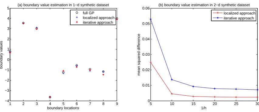
This section numerically compares the two aforementioned solutions for boundary value es-timation. We used the same data set used in Section 4.1.1 and applied the same partitioning scheme for splitting the entire domain into 10 local regions, in between which there are nine boundary locations. We applied the localized estimation method and the iterative block Gauss-Seidel approach for estimatingf(x) at the nine locations, and compared them with the estimated values from a full GP regression. Figure 2-(a) shows the comparison results. The root mean squared difference of the localized estimation to a full GP regression was 0.0775, while that of the iterative approach was 0.1369. Both of the errors are far below the noise parameterσ= 1. The computation time for the estimation was comparable, 0.041328 seconds for the localized method and 0.038071 seconds for the iterative approach.
For another comparison, we generated a synthetic data set in 2-d of 8,000 noisy obser-vations from a zero-mean Gaussian process with an exponential covariance function of scale one and variance 10,
yi =f(xi) +i fori= 1, . . . ,8000,
5 10 15 20 25 30 0
0.01 0.02 0.03 0.04 0.05 0.06
1/h
mean squared difference
(b) boundary value estimation in 2−d synthetic dataset
localized approach iterative approach
1 2 3 4 5 6 7 8 9
−4 −3 −2 −1 0 1 2 3 4 5
boundary locations
boundary values
(a) boundary value estimation in 1−d synthetic dataset
full GP localized approach iterative approach
Figure 2: Comparison of the two proposed methods of boundary value estimation with a full GP regression.
boundary estimation by the localized approach or the iterative approach and the full GP regression prediction. The mean squared differences versus mesh sizehare plotted in Figure 2-(b). Again, the localized approach works better.
4.3 Computation Complexity and Implementation Details
The total computation complexity of our proposed approach is the summation of two com-plexities, one for the constrained GP regressions and the other for the boundary value esti-mation. It isO(SNS3+dSNB3) when the localized estimation approach is used for boundary value estimation, and it is O(SNS3 +d2S2) when the block Gauss-Seidel iteration is used. Since SNS=N andNB is a constant, the complexity isO(N NS2+dS) orO(N NS2+d2S2) respectively.
4.3.1 Evaluation of Integrals for quantities in Equation (20)
The integrals for defining several quantities in equation (20) can be computed effectively using well-established finite element computations. Suppose that Ω ⊂Rd and we use the
Lagrange finite elements of polynomial degreek, where thesth local region Ωsis partitioned into M mesh cells {Km;m= 1, . . . , M} for the finite element approximation. The φs is a column vector of the Lagrange basis functions for the mesh cells,
{φm,j;m= 1, . . . , M, j= 0,1, . . . , J}, and J =
d+k k
.
Φs,0 andΦs,b. For example, whend= 2, Z
Km
λaj1λbj2λcj3 = 2|Km|
a!b!c! (2 +a+b+c)!,
and when d= 3,
Z
Km
λaj1λbj2λjc3λdj4 = 6|Km|
a!b!c!d! (3 +a+b+c+d)!,
where |Km| is the volume of Km. Since φm,j1φm,j2 is also a polynomial functions of λj’s, one can use the previous integration formulas to evaluateRK
mφm,j1φm,j2 and
Z
Ωs
φm,j1φm,j2 =
X
m Z
Km
φm,j1φm,j2. (26)
For the values of Fs, one can take the finite element approximation of fs, where each functionfi infs is approximated by
X
j
α(m,ji) φm,j on Km.
With this approximation, Fs becomes
Z
Ωs
φsfi= X
m Z
Km
φsX
j
αm,j(i) φm,j
=X
m X
j
α(m,ji)
Z
Km
φsφm,j.
The last integral can be computed using (26).
Since φm,j|Γst is a polynomial function of barycentric coordinates with respect to Γst,
Z
Γst
φm,j1|Γstφm,j2|Γjk
can be computed using the integral formulas in barycentric coordinates, facilitating the evaluation ofBs and bs.
4.3.2 Learning Covariance Parameters
By far, our discussions have been made when using fixed parameters (often referred to as hyperparameters in the literature) for the covariance function k(·,·). In this subsection, we discuss how to choose the hyperparameters. Basically, we follow the approach in Park et al. (2011), which has two options, namely choosing different hyperparameters for each local region or choosing the same hyperparameters for all local regions. When different hyperparameters are chosen for each local region, the hyperparameters are estimated by maximizing the local marginal likelihood functions. Specifically, the local hyperparameters, denoted by θs associated with each Ωs, are selected such that they minimize the negative log marginal likelihood:
M Ls(θs) :=−logp(ys;θs) =
ns
2 log(2π) + 1
2log|As|+ 1 2y
0
where As depends on θs. Note that (27) is the marginal likelihood of the standard local kriging model typically seen in geostatistics.
When we want to choose the same hyperparameters applied for all local regions, we choose the hyperparameter θsuch that it minimizes
M L(θ) = S X
s=1
M Ls(θ), (28)
where the summation of the negative log local marginal likelihoods is over all local regions. The above treatment implicitly assumes that the data from each local region are mutually independent. We used the criterion (28) for all numerical comparisons presented below.
5. Numerical Study of Patched GP and Comparison with DDM
In this section, we present the numerical performance of our patched GP method for different tuning parameters, compared to the full GP regression. We also compare our patched GP method with its precursor, the DDM (Park et al., 2011).
5.1 Data Sets and Evaluation Criteria
We considered four data sets: one synthetic data set in 1-d, one synthetic data set in 2-d, and three real spatial data sets both in 2-d. The two synthetic data sets were generated by the R packageRandomField. The first data set in 1-d (hereafter denoted bysynthetic-1d) consists of 6,000 noisy observations from a zero-mean Gaussian process with an exponential covariance function of scale one and variance 10,
yi =f(xi) +i fori= 1, . . . ,6000,
wherexi ∼Uniform(0,10) andi∼ N(0,1) were independently sampled, and the Gaussian process realization f(xi) was simulated by the R package. The synthetic data set in 2-d (hereafter denoted bysynthetic-2d) consists of 8,000 noisy observations from a zero-mean Gaussian process with an exponential covariance function of scale one and variance 10,
yi =f(xi) +i fori= 1, . . . ,8000,
where xi ∼ Uniform([0,6]×[0,6]) and i ∼ N(0,1) were independently sampled, and the Gaussian process realizationf(xi) was simulated by the R package RandomField. The two synthetic data sets were used to show how our proposed method performs, compared to the full GP regression.
−150 −100 −50 0 50 100 150 −80
−60 −40 −20 0 20 40 60 80
longitude
latitude
TCO dataset
−125 −120 −115 −110 −105
−84 −83.5 −83 −82.5 −82 −81.5
longitude
latitude
ICETHICK dataset
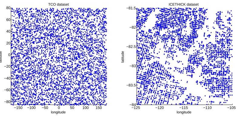
Figure 3: Spatial distribution of the measurements for two real data sets. A dot represent one measurement.
Using the three real spatial data sets, we can compare the computation time and pre-diction accuracy of the patched GP with other methods. We randomly split each data set into a training set containing 90% of the total observations and a test set containing the remaining 10% of the observations. To compare the computational efficiency of methods, we measure two computation times, the training time (including the time for hyperparam-eter learning) and the prediction (or test) time. For comparison of accuracy, we use two measures on the set of the test data, denoted as{(xt, yt);t= 1, . . . , T}, whereT is the size of the test set. The first measure is the mean squared error (MSE)
MSE = 1
T
T X
t=1
(yt−µt)2, (29)
which measures the accuracy of the mean prediction µt at location xt. The second one is the negative log predictive density (NLPD)
NLPD = 1
T
T X
t=1
(yt−µt)2 2σ2t +
1
2log(2πσ
2
t)
, (30)
which considers the accuracy of the predictive variance σt as well as the mean prediction
µt. These two criteria were used broadly in the GP regression literature. A smaller value of MSE or NLPD indicates a better performance.
software (Persson and Strang, 2004). We used the localized estimation presented in Section 4.2.1 for boundary value estimation, and the hyperparameters of a covariance function was obtained by minimizing (28) and was applied for all local regions. All numerical studies were performed on a computer with Intel Xeon Processor W3520 and 6GB memory.
5.2 Performance of Patched GP with Different Tuning Parameters
The patched GP has two tuning parameters, number of local regions S and mesh size h
in finite element approximation. If the number of local regions (S) is one (i.e. there is no split to local regions), the patched GP should converge to a full GP as the mesh size of the patched GP’s finite element approximation goes to zero. In this section we illustrate how the patched GP works for S >1 and different mesh sizes using the data sets described in the previous section.
For synthetic-1d, we uniformly partitioned the domain [0,10] intoS local regions of equal size where S varies over {2,4,6,8,10}. The number of meshes per local region is denoted by M, and it is related to mesh size h, which is the length of an interval mesh. We randomly split 6,000 observations in synthetic-1d into a training data set of 4,500 observations and a test data set of 1,500 observations. For each S and h, we used the training data set to learn the patched GP and a full GP, and compared the mean squared difference of the patched GP and a full GP over the test data set. Figure 4-(a) shows the mean squared difference versusS andh. Regardless ofS, the difference converges to almost zero (aboute−6) ash goes to zero, which implies that the mean prediction of the patched GP becomes very close to that of a full GP even with a large S; this can be qualitatively seen in Figure 4-(b), -(c) and -(d). In other words, the performance of the patched GP does not vary much with the choice ofS although the method with a largerStypically converges faster.
For synthetic-2d, we uniformly partitioned the domain into S local regions of equal size where S varies over {68,47,32,17,10,4}. The number of meshes per local region is denoted byM, and it is related to mesh sizeh, which is the side length of a triangular mesh forsynthetic-2d. We randomly split 8,000 observations in synthetic-2d into a training data of size 6,500 and a test data set of size 1,500. For eachS and h, we used the training data set to learn the patched GP and a full GP, and compared the mean squared difference between the patched GP and the full GP over the test data set. Figure 5 shows the mean squared difference versus S and h. Similar to the 1-d case, the performance of patched GP does not vary much with different S values for the two synthetic data sets.
We also evaluated the performance of the patched GP on the real data sets TCO and
ICETHICK for different values of S and M. As described in Section 5.1, 90% of each data set was randomly chosen and used as a training data set, and the remaining 10% was used for computing the MSE. Figure 6 summarizes the results. The performance of the patched GP did not vary much for different S. If S is large, the overall computation complexity decreases significantly asM decreases. Therefore, in general, a larger S is preferred.
5.3 Comparison with DDM
0 20 40 60
−100
inverse of mesh size (1/h)
mean squared difference
(a) MSE vs. S and h
S=10 S=8 S=6 S=4 S=2
0 2 4 6 8 10
−10 −5 0 5 10
(b) S=10
x
y
training data full GP our method
0 2 4 6 8 10
−10 −5 0 5 10
(c) S=5
x
y
training data full GP our method
0 2 4 6 8 10
−10 −5 0 5 10
x
y
(d) S=2
training data full GP our method
Figure 4: Mean squared difference of the patched GP and a full GP over the test data set forsynthetic-1d; (a) shows the mean squared differences for different S and h
parameter values, and (b)-(d) illustrate the mean predictions of the patched GP and a full GP for differentS’s with fixed 1/h= 3.
5.3.1 Overall Performance
0 200 400 600 800 1000 10−2
10−1 100 101
number of meshes per subdomain (M)
mean squared difference
(a) Deviation from full GP vs. S and M
S=68 S=47 S=32 S=17 S=10 S=4
0 5 10 15 20 25 30
10−2 10−1 100 101
inverse of mesh size (1/h)
mean squared difference
(b) Deviation from full GP vs. S and h
S=68 S=47 S=32 S=17 S=10 S=4
Figure 5: Mean squared difference of the patched GP and a full GP versus S and h for
synthetic-2d
0 500 1000 1500 2000 2500 3000 101
102
number of meshes per subdomain (M)
mean squared error
(a) TCO
0 500 1000 1500 2000 2500 3000 3500 4000 104
105
number of meshes per subdomain (M)
mean squared error
(b) ICETHICK
S=101 S=145 S=212 S=274 S=344
S=32 S=47 S=68
Figure 6: MSE of the patched GP versusS and h forTCOand ICETHICK.
For both methods, we fixed S, S = 145 for TCO, S = 623 for TCO.L2, and S = 47 for
0 50 100 150 200 250 300 0 10 20 30 40 50
train + test time (sec)
MSE
Time v.s. MSE for TCO Dataset
0 50 100 150 200 250 300 2
2.5 3 3.5 4
train + test time (sec)
NLPD
Time v.s. NLPD for TCO Dataset
DDM patched GP
DDM patched GP
0 200 400 600 800 1000
45 50 55
train + test time (sec)
MSE
Time v.s. MSE for TCO.L2 Dataset
0 200 400 600 800 1000
3 3.2 3.4 3.6 3.8 4 4.2 4.4
train + test time (sec)
NLPD
Time v.s. NLPD for TCO.L2 Dataset
DDM patched GP
DDM patched GP
0 50 100 150
0 0.5 1 1.5 2 2.5 3 3.5
4x 10 4
train + test time (sec)
MSE
Time v.s. MSE for ICE Dataset
DDM patched GP
0 50 100 150
6 6.5 7 7.5 8
train + test time (sec)
NLPD
Time v.s. NLPD for ICE Dataset
DDM patched GP
overall prediction accuracy and the total computation time. For DDM, we varied the number of degree of freedoms on a local region boundary from 5 to 30 with step size 5. For each experimental setting, we performed 20 replicated experiments with new random splits of training and test data sets. We randomly split each data set into a training set containing 90% of the total observations and a test set containing the remaining 10% of the observations. The MSEs, NLPDs and the total computation times were averaged to reduce the variation caused by random splits.
Figure 7 shows the MSE and NLPD versus the total computation time for both DDM and patched GP. For shorter computation time, DDM performed better in terms of MSE but patched GP obtained lower MSEs with longer computation time. In terms of NLPD, the DDM was better for TCO and TCO.L2. The NLPD is roughly the squared bias of the predictive mean divided by the predictive variance. Since the patched GP is better than the DDM in MSE, the better NLPD performance of the DDM can be attributed to difference in variance estimation. ForTCO and TCO.L2, the DDM’s variance estimation is sufficiently large to cover most observations. However, the DDM’s variance estimation is sometimes too small, being negative. For example, the DDM produced the negative predictive variances for
ICETHICK, so the resulting NLPDs are imaginary numbers. The issue with DDM regarding possible negative predictive variances has been reported in Pourhabib et al. (2014). The same problem occurred in this numerical example.
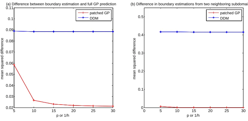
5.3.2 Comparison in Boundary Value Estimation
We compared DDM and patched GP for boundary value estimation. For this comparison, we used the localized estimation approach described in Section 4.2.1 with NB = 50. The comparison was primarily focused on (1) how the boundary estimation of each method on a boundary location is close to the mean prediction of a full GP regression on the same location, and (2) how the boundary estimations of two neighboring local regions on a boundary point are closed to each other. We fixed S = 16 and tried different mesh sizes
h for patched GP and different numbers of the control points placed on each boundary (p) for DDM, which are directly relevant to the performance of boundary estimation. The h
varied over one fifth of a local region size through one thirtieth of a local region size, while
p comparably varied over five through thirty.
We used the whole synthetic-2d data set as a training data set to train both of the methods, and 1,881 test locations were chosen uniformly from local region boundaries. For each test location, we obtained the mean prediction of a full GP regression. The squared differences of the mean prediction of DDM or patched GP to that of a full GP at the test locations are averaged to obtain the mean squared difference. This difference versush orp
is plotted in Figure 8-(a). As h decreases, the boundary estimation of patched GP at the test locations converges to the mean prediction of a full GP regression at the same locations, while the boundary estimation of DDM keeps deviating from a full GP result.
5 10 15 20 25 30 0.02
0.03 0.04 0.05 0.06 0.07 0.08 0.09 0.1 0.11
p or 1/h
mean squared difference
(a) Difference between boundary estimation and full GP prediction
0 5 10 15 20 25 30
0 0.1 0.2 0.3 0.4 0.5
p or 1/h
mean squared difference
(b) Difference in boundary estimations from two neighboring subdomains
patched GP DDM
patched GP DDM
Figure 8: Accuracy of Boundary Estimation.
patched GP are almost zero, while those for DDM are significantly non-zero relative to those of patched GP.
6. Numerical Comparison with Other State-of-The-Art methods
This section compares patched GP with other state-of-the-art methods. Section 6.1 con-tains the comparison to several localized approaches for GP regression, while Section 6.2 contains the comparison to the Gaussian Markov random field approach to the GP regres-sion (Lindgren et al., 2011).
6.1 Comparison with Other Local GP Methods
In this section, we compare patched GP with other localized approaches for GP regression, including BCM (Tresp, 2000), PIC (Snelson and Ghahramani, 2007), and RBCM (Deisen-roth and Ng, 2015); we used the author’s implementation of BCM and implemented RBCM and PIC with matlab by ourselves. We used three real data setsTCO,TCO.L2andICETHICK
to compare the MSEs and NLPDs of the approaches versus the total computation time, which includes the time for hyperparameter learning, model learning and prediction. We used the squared exponential covariance function and used the whole training data set to choose hyperparameters for all of the compared methods. For patched GP, we fixedS= 145 forTCO,S= 623 forTCO.L2, andS= 47 forICETHICK, and the number of meshes per local region was varied from 5 to 40 with step size 5. For BCM and RBCM, we varied the number of local experts M ∈ {100,150,200,250,300,600} forTCO,M ∈ {50,100,150,200,250,300}
forTCO.L2, andM ∈ {50,100,150,200,250,300}forICETHICK. For PIC, we varied the total number of local regions m∈ {100,150,200,250,350} forTCO,m ∈ {100,200,300,400,600}
in-ducing inputs (M ∈ {100,150,200,250,300,400,500,600,700}) for all of the data sets. We used the k-means clustering for splitting training data for both of BCM, RBCM, and PIC.
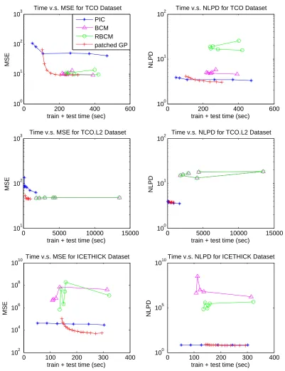
Figure 9 shows the logarithms of MSEs and NLPDs versus total computation times for the three data sets. For TCO data set, the BCM, RBCM, and patched GP obtained more accurate prediction than the PIC, and the patched GP was computationally more efficient than the BCM and RBCM. For TCO.L2data set, the patched GP uniformly outperformed other competing methods, scaling better than BCM and RBCM and achieving better MSE than the PIC. It is interesting to see that BCM is almost identically performing as the RBCM when N is so large like in TCO.L2 data set. For ICETHICK data set, the PIC and patched GP obtained more accurate prediction than the BCM and the RBCM. Please note that the training data are quite densely spread over the whole domain for TCO while the training data are sparse for some local regions in ICETHICK. The patched GP worked well for both of the cases, while the PIC worked better for the sparse case and the BCM worked better for the dense case. The RBCM has shown much better results than the BCM for the sparse case but it is not better than the patched GP and PIC. The PIC combines a global model with local models, which may help to improve the performance for the sparse case.
6.2 Comparison with GMRF
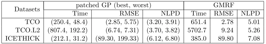
In this section, we compare patched GP with the Gaussian Markov random field approach to the GP regression (Lindgren et al., 2011, GMRF), which was reported to scale great with massive data set; we implemented the GMRF with matlab. The major checkpoints of this comparison are the scalability and prediction accuracy. We used three real data sets of different sizes, ICETHICK (N = 32,813), TCO (N = 48,311) and TCO.L2 (N = 182,591) to compare the MSEs, NLPDS, and computation time of the approaches. In this comparison, we used the exponential covariance function, since the GMRF does not work with the squared exponential covariance function used for the other comparisons; at least, the construction of the precision matrix for Gaussian Markov random field is not straightforward. The GMRF does not have any tuning parameters, and the hyperparameter learning of the GMRF was performed using 5% of the training data; the MSE performance did not change much as the percentage increases, so we chose the smallest percentage to obtain the smallest computation time. For patched GP, we presented the results with the combinations of tuning parameters that obtain the best RMSE and the worst RMSE. To be specific, we fixedS = 145 forTCO,S = 47 forICETHICK, and S = 623 forTCO.L2, while the number of meshes per local region was varied from 5 to 40 with step size 5.
0 200 400 600 100
101 102 103
train + test time (sec)
MSE
Time v.s. MSE for TCO Dataset
0 200 400 600
100 101 102
train + test time (sec)
NLPD
Time v.s. NLPD for TCO Dataset
PIC BCM RBCM patched GP
0 5000 10000 15000
101 102 103
train + test time (sec)
MSE
Time v.s. MSE for TCO.L2 Dataset
0 5000 10000 15000
100 101 102
train + test time (sec)
NLPD
Time v.s. NLPD for TCO.L2 Dataset
0 100 200 300 400
102 104 106 108 1010
train + test time (sec)
MSE
Time v.s. MSE for ICETHICK Dataset
0 100 200 300 400
100 105 1010
train + test time (sec)
NLPD
Time v.s. NLPD for ICETHICK Dataset
Datasets patched GP (best, worst) GMRF
Time RMSE NLPD Time RMSE NLPD
TCO (250.4, 48.4) (2.85, 5.75) (3.20, 3.91) 651.4 2.78 5.01
TCO.L2 (807.4, 192.2) (6.74, 7.31) (3.70, 3.82) 5702.7 9.24 5.26
ICETHICK (212.1, 31.2) (89.30, 199.33) (6.12, 6.80) 385.0 89.80 7.08
Table 1: Performance comparison of the patched GP with GMRF: the time unit used is second.
7. Conclusion
We developed a method for solving a Gaussian process regression with constraints on a do-main boundary and also developed a solution approach based on a finite element method. The method is then applied to local GP regressions as a building block to develop the patched GP method as a computationally efficient solver of a large-scale Gaussian process regression or spatial kriging problem. The patched GP solves two issues of the simple local GP approaches, namely the inaccuracy and inconsistency of prediction on the boundaries of neighboring local regions. Comparing with its precursor DDM, the patched GP has an im-proved way of considering the constraints related to the boundary regions. Both methods reformulate the GP regression as an optimization problem, the patched GP method im-proves DDM by rewriting the optimization problem in a function space and using the finite element methods to solve the required integrals arising from the solution of the minimization problem. The patched GP method is mathematically more elegant and its competitiveness to existing methods is demonstrated through numerical studies.
Acknowledgments
The authors thank the reviewers for constructive comments. The authors also thank An-ton Schwaighofer at Microsoft for sharing the BCM implementation. Chiwoo Park was supported by grants from the National Science Foundation (CMMI-1334012) and the Air Force Office of Scientific Research (FA9550-13-1-0075). Jianhua Z. Huang was supported by grants from the National Science Foundation (DMS-1208952) and the Air Force Office of Scientific Research (FA9550-13-1-0075).
Appendix A. Proof of Proposition 1
Note that [L2(Ω)]N is a Hilbert space with the following inner product (u,v) =
Z
Ω u0v.
We define a bi-linear form on [L2(Ω)]N bya: [L2(Ω)]N ×[L2(Ω)]N →R,
a(u,v) = (Au,v) = Z
Ω
a linear functional c: [L2(Ω)]N →Ras
c(u) = Z
Ω f0u,
and defineJ(u) = 12a(u,u)−c(u). Since Ais a N×N (real) positive definite matrix, the bi-linear forma(u,v) is symmetric and positive. Letα be the smallest eigenvalue ofA. We have that
a(u,u)≥α||u||2, ∀u∈[L2(Ω)]N.
Therefore, the bi-linear form a is coercive. It follows from Ern and Guermond (2004, Proposition 2.4) that, usatisfiesa(u,v)−c(v) = 0 for everyv ∈[L2(Ω)]N if and only if it minimizesJ(u) over u∈[L2(Ω)]N. Note that the coercivity of the bi-linear formacan be interpreted as a strong convexity property of the functionalJ(u), which makes the problem have a unique optimal solution (Ern and Guermond, 2004, Lemma 2.2).
Appendix B. Proof of Proposition 2
We have already proven that a(u,v) = RΩu0Av is coercive, symmetric and positive for
u,v ∈[L2(Ω)]N in the proof of Proposition 1. The same result holds for u,v∈Hb because
Hb⊂[L2(Ω)]N. SinceHb is a Hilbert space, solving the minimization problem is equivalent to solving the integral equation (8) by Ern and Guermond (2004, Proposition 2.4).
References
Sudipto Banerjee, Alan E Gelfand, Andrew O Finley, and Huiyan Sang. Gaussian predictive process models for large spatial data sets. Journal of the Royal Statistical Society: Series B (Statistical Methodology), 70(4):825–848, 2008.
Tao Chen and Jianghong Ren. Bagging for Gaussian process regression. Neurocomputing, 72(7):1605–1610, 2009.
Noel Cressie and Gardar Johannesson. Fiexed rank kriging for very large spatial data sets.
Journal of Royal Statistical Society, Series B, 70:209–226, 2008.
Paul J Curran and Peter M Atkinson. Geostatistics and remote sensing.Progress in Physical Geography, 22(1):61–78, 1998.
Marc Peter Deisenroth and Jun Wei Ng. Distributed Gaussian processes. In Proceedings of the 32 nd International Conference on Machine Learning, pages 1–10, 2015.
A. Ern and J.L. Guermond. Theory and practice of finite elements. Springer Verlag, 2004. ISBN 0387205748.
Thore Graepel. Solving noisy linear operator equations by Gaussian processes: Application to ordinary and partial differential equations. In International Workshop on Machine Learning, volume 20, page 234, 2003.
Robert B Gramacy and Daniel W Apley. Local Gaussian process approximation for large computer experiments. Journal of Computational and Graphical Statistics, pages 561– 578, 2015.
Robert B Gramacy and Herbert KH Lee. Bayesian treed Gaussian process models with an application to computer modeling. Journal of the American Statistical Association, 103 (483), 2008.
Cari G Kaufman, Mark J Schervish, and Douglas W Nychka. Covariance tapering for likelihood-based estimation in large spatial data sets. Journal of the American Statistical Association, 103(484):1545–1555, 2008.
Finn Lindgren, H˚avard Rue, and Johan Lindstr¨om. An explicit link between Gaussian fields and Gaussian markov random fields: the stochastic partial differential equation approach. Journal of the Royal Statistical Society: Series B (Statistical Methodology), 73 (4):423–498, 2011.
David JC MacKay. Introduction to Gaussian processes. In C. M. Bishop, editor,Neural net-works and machine learning, volume 168 ofNATO ASI Series F Computer and Systems Sciences, pages 133–166. Springer Verlag, 1998.
A Mahmood, DJ Lynch, and LD Philipp. A fast banded matrix inversion using connectivity of schur’s complements. InIEEE International Conference on Systems Engineering, pages 303–306. IEEE, 1991.
Duy Nguyen-Tuong, Jan R Peters, and Matthias Seeger. Local Gaussian process regres-sion for real time online model learning. In Advances in Neural Information Processing Systems, pages 1193–1200, 2009.
Chiwoo Park, Jianhua Z. Huang, and Yu Ding. Domain decomposition approach for fast Gaussian process regression of large spatial datasets. Journal of Machine Learning Re-search, 12:1697–1728, May 2011.
Per-Olof Persson and Gilbert Strang. A simple mesh generator in matlab. SIAM review, 46(2):329–345, 2004.
Arash Pourhabib, Faming Liang, and Yu Ding. Bayesian site selection for fast Gaussian process regression. IIE Transactions, 46(5):543–555, 2014.
C. E. Rasmussen and Z. Ghahramani. Infinite mixtures of Gaussian process experts. In
Advances in Neural Information Processing Systems 14, pages 881–888. MIT Press, 2002.
C.E. Rasmussen and C.K.I. Williams. Gaussian Processes for Machine Learning. The MIT Press, 2005.
Huiyan Sang and Jianhua Z. Huang. A full-scale approximation of covariance functions for large spatial data sets. Journal of Royal Statistical Society, Series B, 74:111–132, 2012.
Matthias Seeger, Christopher K. I. Williams, and Neil D. Lawrence. Fast forward selection to speed up sparse Gaussian process regression. In International Workshop on Artificial Intelligence and Statistics 9. Society for Artificial Intelligence and Statistics, 2003.
Edward Snelson and Zoubin Ghahramani. Sparse Gaussian processes using pseudo-inputs. In Advances in Neural Information Processing Systems 18, pages 1257–1264. MIT Press, 2006.
Edward Snelson and Zoubin Ghahramani. Local and global sparse Gaussian process approx-imations. In International Conference on Artifical Intelligence and Statistics 11, pages 524–531. Society for Artificial Intelligence and Statistics, 2007.
Michael L Stein. Interpolation of spatial data: some theory for kriging. Springer Science & Business Media, 2012.
Florian Steinke and Bernhard Sch¨olkopf. Kernels, regularization and differential equations.
Pattern Recognition, 41(11):3271–3286, 2008.
Volker Tresp. A bayesian committee machine.Neural Computation, 12(11):2719–2741, 2000.
Jarno Vanhatalo and Aki Vehtari. Modelling local and global phenomena with sparse Gaussian processes. In the 24th Conference on Uncertainty in Artificial Intelligence, page 571578. Association for Uncertainty in Artificial Intelligence, 2008.