Combined
`
1and Greedy
`
0Penalized Least Squares
for Linear Model Selection
∗Piotr Pokarowski [email protected]
Faculty of Mathematics, Informatics and Mechanics University of Warsaw
Banacha 2, 02-097 Warsaw, Poland
Jan Mielniczuk [email protected]
Faculty of Mathematics and Information Science Warsaw University of Technology
Koszykowa 75, 00-662 Warsaw, Poland Institute of Computer Science
Polish Academy of Sciences
Jana Kazimierza 5, 01-248 Warsaw, Poland
Editor:Tong Zhang
Abstract
We introduce a computationally effective algorithm for a linear model selection consisting of three steps: screening–ordering–selection (SOS). Screening of predictors is based on the thresholded Lasso that is`1penalized least squares. The screened predictors are then fitted using least squares (LS) and ordered with respect to their |t| statistics. Finally, a model is selected using greedy generalized information criterion (GIC) that is`0 penalized LS in a nested family induced by the ordering. We give non-asymptotic upper bounds on error probability of each step of the SOS algorithm in terms of both penalties. Then we obtain selection consistency for different (n, p) scenarios under conditions which are needed for screening consistency of the Lasso. Our error bounds and numerical experiments show that SOS is worth considering alternative for multi-stage convex relaxation, the latest quasiconvex penalized LS. For the traditional setting (n > p) we give Sanov-type bounds on the error probabilities of the ordering–selection algorithm. It is surprising consequence of our bounds that the selection error of greedy GIC is asymptotically not larger than of exhaustive GIC.
Keywords: linear model selection, penalized least squares, Lasso, generalized information criterion, greedy search, multi-stage convex relaxation
1. Introduction
Literature concerning linear model selection has been lately dominated by analysis of the
least absolute shrinkage and selection operator (Lasso) that is `1 penalized least squares
for the ’large p - small nscenario’, where n is number of observations andp is number of all predictors. For a broad overview of the subject we refer to B¨uhlmann and van de Geer (2011). It is known that consistency of selection based on the Lasso requires strong regularity
of an experimental matrix namedirrepresentable conditionswhich are rather unlikely to hold in practice (Meinshausen and B¨uhlmann, 2006; Zhao and Yu, 2006). However, consistency of the Lasso predictors or consistency of the Lasso estimators of the linear model parameters is proved under weaker assumptions such as therestricted isometry property(RIP). The last condition means that singular values of normalized experimental submatrices corresponding to small sets of predictors are uniformly bounded away from zero and infinity. Under those more realistic conditions and provided that a certain lower bound on the absolute values of model parameters calledbeta-min condition holds, the Lasso leads to consistent screening, that is the set of nonzero Lasso coefficientsS contains with large predetermined probability the uniquely defined true modelT. This property explains B¨uhlmann’s suggestion that one should interpret the second ’s’ in ’Lasso’ as ’screening’ rather than ’selection’ (see discussion of Tibshirani, 2011) and the task is now to remove the spurious selected predictors. To this aim two-stage procedures as the adaptive or the thresholded Lasso have been proposed (cf. Zou, 2006; Huang et al., 2008; Meinshausen and Yu, 2009; Zhou, 2009, 2010; van de Geer et al., 2011). They yield selection consistency under strong version of the beta-min condition and without such strengthening tend to diminish the number of selected spurious predictors, but, similarly to the Lasso they yield screening consistency only. Alternative approaches require minimization of least squares (LS) penalized by quasiconvex functions that are closer to the `0 penalty then `1 (Fan and Li, 2001; Zou and Li, 2008; Zhang,
2010a,b; Zhang and Zhang, 2012; Huang and Zhang, 2012; Zhang, 2013; Wang et al., 2014). These methods lead to consistent selection under RIP and considerably weaker version of the beta-min condition, nevertheless are more computationally demanding.
Regularization is required when a model matrix is not a full rank or whenn < p, but for the traditional regression when an experimental plan is of full rank andn > pit is possible to construct a computationally effective and selection consistent two-stage ordering–selection
(OS) procedure, as follows. First, a full modelF using LS is fitted, predictors are ordered with respect to their|t|statistics from the fit and finally, a submodel ofF in a nested family pertaining to the ordering is selected using thresholding as in Rao and Wu (1989), Bunea et al. (2006) orgeneralized information criterion(GIC) as in Zheng and Loh (1995). The OS algorithm can be treated asgreedy`0 penalized LS because it requires computing a criterion
function for 2p models only instead of all 2p models. Frequently, sufficient conditions on an experimental plan and a vector of true coefficients for consistency of such procedures are stated in terms of theKullback-Leibler divergence(KL) of the true model from models which lack at least one true predictor (Zheng and Loh, 1995; Shao, 1998; Chen and Chen, 2008; Casella et al., 2009; P¨otscher and Schneider, 2011; Luo and Chen, 2013). In particular, a bound on the probability of selection error in Shao (1998) closely resembles the Sanov theorem in information theory on bounds of probability of a non-typical event using the KL divergence.
selection consistency for different (n, p) scenarios under weak conditions which are sufficient for screening consistency of the Lasso. Our assumptions allow for strong correlation between predictors, in particular replication of spurious predictors is possible.
The SOS algorithm is an improvement of the new version of the thresholded Lasso and turns out to be a promising competitor to multi-stage convex relaxation(MCR), the latest quasiconvex penalized LS (Zhang, 2010b, 2013). The condition on correlation of predictors assumed there seems to be stronger than ours, whereas the beta-min condition may be weaker (Section 5). In our simulations for |T| npscenario, SOS was faster and more accurate than MCR (Section 8).
For casen > pwe also give a bound on probability of selection error of the OS algorithm. Our bound in this case is more general than in Shao (1998) as we allow ordering of predictors,
p =pn → ∞ , |T|=|Tn| → ∞ or the GIC penalty may be of order n (Theorem 2). It is
surprising consequence of Theorems 1-2 that the probability of selection error of greedy GIC is asymptotically not larger than of exhaustive GIC. Thus employment of greedy search dramatically decreases computational cost of l0 penalized LS minimization without
increasing selection error probability.
As a by-product we obtained a strengthened version of the nonparametric sparse oracle inequality for the Lasso proved by Bickel et al. (2009) and, as its consequence, more tight bounds on prediction and estimation error (Theorem 4). We simplified and strengthened an analogous bound for the thresholded Lasso given by Zhou (2009, 2010) (Theorem 1 part T1). It is worth noticing that all results are proved simultaneously for two versions of the algorithm: for the Lasso used in practice when a response is centered and predictors are standardized as well as for its formal version for which an intercept corresponds to a dummy predictor.
The paper is organized as follows. In Section 2 the SOS algorithm is introduced and in Section 3 we study properties of geometric characteristics pertaining to an experimental matrix and a vector of coefficients which are related to identifiability of a true model. Section 4 contains our main results that is bounds on selection error probabilities for the SOS and OS algorithm. In Section 5 we briefly discuss the MCR algorithm and compare error bounds for SOS and MCR. Section 6 treats properties of post-model selection estimators pertaining to SOS and MCR. Section 7 contains improved bounds on the Lasso estimation and prediction. Section 8 presents a simulational study. Concluding remarks are given in Section 9. Appendix contains detailed proofs of the stated results.
2. Selection Algorithm
2.1 Linear Regression Model Parametrizations
We consider a general regression model of real-valued responses having the following struc-ture
yi =µ(xi.) +εi, i= 1,2, . . . , n,
whereε1, . . . , εn are iidN(0, σ2),xi.∈Rp, and p=pn may depend onn. In a vector form
we have
y=µ+ε, (1)
whereµ= (µ(x1.), . . . , µ(xn.))T, ε= (ε1, . . . , εn)T and y= (y1, . . . , yn)T.
Let X = [x1., . . . , xn.]T = [x1, . . . , xp] be the n×p matrix of experiment. We consider two linear parametrizations of (1). The first parametrization is:
µ=α∗+Xβ∗, (2)
where α∗ ∈ R is an intercept and β∗ ∈ Rp is a vector of coefficients corresponding to predictors. The second parametrization is
µ=Xβ∗, (3)
where the intercept is either set to 0 or is incorporated into vectorβ∗and treated in the same way as all other coefficients in the linear model. In order to treat both parametrizations in the same way we write µ= ˜Xβ˜∗ where, with 1n denoting a column of ones, ˜X = [1n, X]
and ˜β∗= (α∗, β∗T)T in the case of (2) and ˜X =X and ˜β∗=β∗ in the case of (3). We note
that (3) is convenient for theoretical considerations and simulations on synthetic data, but (2) is natural for real data applications and occurs as a default option in popular statistical software.
LetJ ⊆ {1,2, . . . , p}=F be an arbitrary subset of the full modelF and|J|the number of its elements,XJ is a submatrix ofXwith columns having indices in J,βJ is a subvector
of β with columns having indices in J. Moreover, let ˜XJ = [1n, XJ] and ˜βJ = (α, βTJ)T in
the case of (2) or ˜XJ =XJ and ˜βJ =βJ in the case of (3). ˜HJ will stand for a projection matrix onto the subspace spanned by columns of ˜XJ. Linear model pertaining to predictors
being columns of XJ will be frequently identified as J. We will also denote by T = Tn a
true model that is a model such that T = supp(β∗) ={j ∈ F :βj∗ 6= 0} for some β∗ such thatµ= ˜Xβ˜∗. The uniqueness of T and β∗ for a givennwill be discussed in Section 3.
2.2 Practical and Formal Lasso
of the Lasso. Let H0 be an n×n projection matrix, where H0 is specified as a vector
centering matrix In−1n1Tn/nin the case of the applied version of the Lasso pertaining to
parametrization (2) and the identity matrix In for the formal Lasso corresponding to (3).
Moreover, let
D= diag(||H0xj||)pj=1, X0=H0XD−1, X0 = [x01, . . . , x0p], y0=H0y (4) and θ∗ =Dβ∗,µ0 =H0µ. For estimation of β∗, data (X0, y0) will be used. Note that for
the first choice of orthogonal projection in the definition of X0 columns in X are normal-ized by their norms whereas for the second they are standardnormal-ized (centered and divided by their standard deviations). Consider the case of (2) and denote by H0J projection onto
sp{(H0xj)j∈J}. Observe that as sp{1n,(xj)j∈J} = sp{1n} ⊕sp{(H0xj)j∈J} and
conse-quently ˜HJ =H0J+1n1Tn/n, we have that
In−H˜J = (In−H0J)H0. (5)
The above equality trivially holds also in the case of (3). For a = (aj) ∈ Rk, let |a| = Pk
j=1|aj| and ||a|| = ( Pk
j=1a2j)1/2 be `1 and `2 norms,
respectively. AsJmay be viewed as sequence of zeros and ones onF,|J|denotes cardinality of J.
General form of the Lasso estimator ofβ is defined as follows
ˆ
β = argminβ{||H0(y−Xβ)||2+ 2rL|Dβ|}=D−1(argminθ{||y0−X0θ||2+ 2rL|θ|}), (6)
where a parameter rL = rnL is a penalty on l1 norm of a potential estimator of β. Thus
in the case of parametrization (2) the Lasso estimator of β may be defined without using extended matrix ˜X by applying H0 to y −Xβ that is by centering it. In the case of parametrization (3)H0 =In and the usual definition of the Lasso used in formal analysis
is obtained. We remark that the approaches used in theoretical considerations for which columns ofX are not normalized as in B¨uhlmann and van de Geer (2011) or Zhang (2013) formally correspond to (6) with H0 =In andD=dIp, whered= max1≤j≤p||xj||.
Note that in the case of parametrization (2) ˆβ is subvector corresponding to β of the following minimizer
argminβ˜{||y−X˜β˜||2+ 2rL|Dβ|}= argminα,β{||y−α1n−Xβ||2+ 2rL|Dβ|}, (7)
where the equality of minimal values of expressions appearing in (6) and (7) is obtained when the expression||y−α1n−Xβ||2 is minimized with respect toα for fixedβ. However,
omitting centering projection H0 in (6) when the first column of X consists of ones and corresponds to intercept, leads to lack of invariance of ˆβ when the data are shifted by a constant and yields different estimates that those used in practice. This is a difference between the Lasso and the LS estimator: LS estimator has the same form regardless of which of the two parametrizations (2) or (3) is applied. Using (5) we have for the LS estimator ˆβLS
J in model J that the sum of squared residuals for the projection ˜Hy equals
RJ =||(In−H˜J)y||2=||(In−H0J)y0||2 =||y0−X0JθˆLSJ ||2 (8)
and
ˆ
2.3 Implementation of the Screening–Ordering–Selection Scheme
The SOS algorithm which is the main subject of the paper is the following implementation of the SOS scheme.
Algorithm(SOS) Input: y, X and rL, b, r.
Screening. Compute the Lasso estimator ˆβ=D−1θ,ˆ θˆ= (ˆθ1, . . .θˆp)T with a penalty
parameterrL and setS0 ={j:|θˆj|> b}, B=b(|S0| ∨1)1/2, S1 ={j :|θˆj|> B}.
Ordering. Fit the model S1 by ordinary LS and order predictors ˆO = (j1, j2, . . . , j|S1|)
using values of corresponding squared tstatisticst2j1 ≥t2j2 ≥. . .≥t2j
|S1|.
Selection. In the nested family G={∅,{j1},{j1, j2}, . . . , S1} choose a model ˆT ≡TˆS 1,Oˆ
according to thegeneralized information criterion (GIC) ˆT = argminJ∈G{RJ+|J|r},
wherer=rn is a penalty pertaining to GIC.
Output: TˆSOS = ˆT, ˆβSOS = ˆβTLSˆ .
The OS algorithm is intended for the case p < nand is a special case of SOS for which
S1 is taken equal toF.
We note that empty set in the definition of G corresponds to µ = 0 in the case of parametrization (3) andµ=α∗ in the case of (2). It is easy to check also that
t2j n− |S1|
= RS1\{j}−RS1
RS1
, (9)
thus ordering with respect to decreasing values of (t2j) in the second step of the procedure is the same as ordering of (RS1\{j}) in decreasing order.
2.4 Computational Complexity of the SOS Algorithm
There are many approximate algorithms for the Lasso estimator (6) as quadratic program solvers or coordinate descent in Friedman et al. (2010). The popular LARS method proposed in Efron et al. (2004) can be used to compute exactly, in finitely many steps, the whole Lasso regularized solution path which is piecewise linear with respect to rL. It has been shown
recently in Mairal and Yu (2012) that, in the worst case, the number of linear segments of this path is exactly (3p+ 1)/2, so the overall computational cost of the Lasso isO(3ppn), see Rosset and Zhu (2007). Hence, by the most popular criterion of computational complexity LARS does not differ from, for example, an exhaustive search for the `0 penalized LS problem. However, experience with data suggests that the number of linear segments of the LARS regularization path is typically O(n), so LARS execution requires O(npmin(n, p)) flops, see Rosset and Zhu (2007) and B¨uhlmann and van de Geer (2011), chapter 2.12. Thus taking into account the result in Mairal and Yu (2012) on uniform approximation of the Lasso regularization paths, for typical data set the Lasso may be considered computationally efficient (cf. also discussion on the page 7 in Zhang (2013)).
In Section 4 we will discuss conditions on X and βT∗, under whichS1 includes a unique
QR decomposition of the matrix X0S1. Computing (RJ)J∈G in the selection step demands
also only one QR decomposition of X0S1 with columns ordered according to ˆO. Indeed,
let X0S1 = QW, where an orthogonal matrix Q = [q1, . . . , q|S1|]. The following iterative
procedure can be used
R∅=||y0||2; for k= 1, . . . ,|S1| do R{1,...,k} =R{1,...,k−1}−(qTky0)2 endfor.
Observe, that from (9) the ordering part demands GIC only for |S1| models that is for S1 \ {j}, j ∈ S1. Thus two last parts of the SOS algorithm or, equivalently, the OS
algorithm demands GIC only for 2|S1|models instead of all 2|S1| and we can call it greedy `0 penalized LS.
We conclude that the SOS algorithm is computationally efficient and the most time expensive part of it is the screening. The same conclusion follows from our simulations described in Section 8.
3. A True Model Identifiability
In this section we consider two types of linear model characteristics which will be used to quantify the difficulty of selection or, equivalently, a true model identifiability problem, and we study the interplay between them.
3.1 Kullback-Leibler Divergences
LetT be given true model that isT ⊆F such thatµ= ˜Xβ˜∗ = ˜XTβ˜T∗ andT = supp(βT∗) =
{j∈F :β∗j,T 6= 0}. ForJ ⊆F define
δ(T kJ) =||(In−HJ˜ ) ˜XTβ˜T∗||2.
In view of (5) we obtain
δ(T kJ) =||(In−H0J)H0X˜Tβ˜T∗||2 =||(In−H0J)H0XTβT∗||2 =||(In−H0J)X0TθT∗||2. (10)
Let KL( ˜βT∗ kβ˜J) =Eβ˜∗
Tlog(fβ˜
∗
T/fβ˜J) be the Kullback-Leibler divergence of the normal density fβ˜∗
T of N( ˜XT ˜
βT∗, σ2In) from the normal density fβ˜J of N( ˜XJβJ˜ , σ2In). Let Σ = X0TX0 be acoherence matrixif H0 is the identity matrix and a correlation matrix ifH0 =
In−1n1Tn/n. Let ΣJ stands for a submatrix of Σ with columns having indices in J and
letλmin(ΣJ), λmax(ΣJ) denote extremal eigenvalues of ΣJ. The following proposition lists
the basic properties of the parameter δ. Observe also that δ(T k J) is a parameter of non-centrality of χ2 distribution of RJ that is RJ ∼χ2n−|J|(δ(T kJ)).
Proposition 1
(i) δ(T kJ) = 2σ2min
˜ βJ
KL( ˜βT∗ kβJ˜ ) = 2σ2min
˜ βJ
KL( ˜βJ kβ˜T∗).
(ii) δ(T kJ) = min
θJ
[X0,T\J, X0,J]
θ∗T\J θJ
2
The following scaled Kullback-Leibler divergence will be employed in our main results in Section 4.
δ(T, s) = min
j∈T,J⊇T,|J|≤sδ(T
kJ\ {j}).
This coefficient was previously used to prove selection consistency in Zheng and Loh (1995); Chen and Chen (2008); Luo and Chen (2013) and to establish asymptotic law of post-selection estimators in P¨otscher and Schneider (2011). Similar coefficients appear in proofs of selection consistency in Shao (1998) and Casella et al. (2009). Obviously, δ(T, s) is a nonincreasing function of s.
Identifiability of a true model is stated in the proposition below in terms of
δ(T) = min
J+T ,|J|≤|T|
δ(T kJ).
Proposition 2 There exists at most one true model T such thatδ(T)>0.
Assume by contradiction thatT0 is a different true model, that is we haveT0 = supp( ˜β) for some ˜β such thatµ= ˜Xβ˜. Then by symmetry we can assume|T| ≤ |T0|. Hence|T0\T|>0 and δ(T0)≤δ(T0 kT) = 0.
It is easy to see that if δ(T) >0 then columns of XT are linearly independent and,
conse-quently, there exists at most one ˜βT∗ such thatµ= ˜XTβ˜T∗.
In Section 4.2 we infer identifiability of a true model T from Proposition 2 and the following inequality
δ(T, p)≤δ(T). (12)
Indeed, for any J such that J +T and |J| ≤ |T|there existsj ∈T such thatJ ⊆F \ {j}.
Thus we obtainδ(T kF\ {j})≤δ(T kJ) and minimizing both sides yields (12).
3.2 Restricted Eigenvalues
ForJ ⊆F, ¯J =F \J and c >0 let
κ2(J, c) = min
ν6=0,|νJ¯|≤c|νJ|
νTΣν
νJTνJ and κ
2(s, c) = min
J:|J|≤sκ(J, c).
Both coefficients will be calledrestricted eigenvalues of Σ. Observe that
κ2(J, c) = min
ν6=0,|νJ¯|≤c|νJ|
||X0ν||2
||νJ||2 =ν6=0,|minν ¯
J|≤c|νJ|
||X0νJ−X0νJ¯||2
||νJ||2 . (13)
The coefficientκ(s, c) is a modified version of an index introduced in Bickel et al. (2009). Modification consists in replacingXappearing in the original definition byX0and omitting
the term n−1/2. Pertaining parameters for a fixed set of predictors J and their various modifications were introduced and applied to bound the Lasso errors by van de Geer and B¨uhlmann (2009).
In order to study relations between sparse and restricted eigenvalues we set
κ2(J,0) = min
ν6=0,supp(ν)⊆J νTΣν
νTν and κ
2(s,0) = min J:|J|≤sκ
Note that ifX0is defined in (4) or in remark below (6) applies we have that max1≤j≤p||x0j|| ≤
1. Thus from Rayleigh-Ritz theorem we have
κ2(J,0) =λmin(ΣJ)≤
tr(ΣJ)
|J| ≤1∧λmax(ΣJ). (14)
The upper bound above equals 1 when the columns are normalized or standardized. Note thatκ(J, c) andκ(s, c) are nonincreasing functions of both arguments. Moreover,κ2(J, c)≤
κ2(J,0) and κ2(s, c) ≤κ2(s,0). This holds in view of an observation that for any fixed J
and c > 0, any ν such that supp(ν) ⊆J satisfies ν =νJ and thus |νJ¯| ≤c|νJ|. It is easy
to show also that κ2(J, c) → κ2(J,0) and κ2(s, c) → κ2(s,0) monotonically when c → 0+. Another less obvious bound, which is used in the following is stated below.
Proposition 3 For any s∈Nand c >0
κ2(s, c)≤(bcc+ 1)κ2((bcc+ 1)s,0).
Condition κ(s, c) >0 imposed on matrix X is called restricted eigenvalue condition in Bickel et al. (2009) for their slightly different κ. Proposition 3 generalizes an observation there (p. 1720) that if the restricted eigenvalue condition holds for c ≥1, then all square submatrices of Σ of size 2s are necessarily positive definite. Indeed, the proposition above implies thatκ(2s,0)>0 from which the observation follows. Positiveness of κ(T, c) which due to the restriction on vectorsν over which minimization is performed can hold even for
p > n, is a certain condition on weak correlation of columns. This condition, which will be assumed later, is much less stringent thanκ(|T|, c)>0, as it allows for example replication of columns belonging to the complement of T. Moreover κ(T, c) > 0 for c ≥ 1 implies identifiability of a true model.
Proposition 4 There exists at most one true model T such thatκ(T,1)>0.
It follows that if κ(T,1)>0, then columns of XT are linearly independent and,
conse-quently, there exists at most one ˜βT∗ such thatµ= ˜XTβ˜T∗.
The followingκ−δinequalitiesfollow from the Propositions 1 (ii) and the Proposition 3. We set θmin∗ = minj∈T|θ∗j|and t=|T|.
Proposition 5 We have
κ2(T,3)θmin∗2 ≤δ(T, t) (15)
and
κ2(t,3)θmin∗2 ≤4δ(T,4t). (16)
4. Error Bounds for the SOS and OS Algorithms
4.1 Error Bounds for SOS
LetSnbe a family of models having no more thanspredictors wheresis defined below and Tn={S ∈ Sn :S ⊇T} consists of all true models in Sn. Observe that|Tn|=Psk=0−t p−kt
. Moreover, let OS1 denote a set of all correct orderings of S1 that is orderings such that
all true variables in S1 precede the spurious ones. To simplify notation set δs = δ(T, s), δt =δ(T, t) andκ =κ(T,3). We also define two constants c1 = (3 + 6√2)−1 ≈0.087 and
c2 = (6 + 4√2)−1≈0.086. We assume for the remaining part of the paper thatp≥t+ 1≥2 as boundary cases are easy to analyze. Moreover, we assume the following condition which ensures that the size ofS1 defined in the first step of the SOS algorithm does not exceedn
with large probability and consequently LS could be performed on data (y0, X0S1). It states
that
s=s(T) =t+bt1/2κ−2c ≤n. (17)
Theorem 1 (T1) If for somea∈(0,1) 8a−1σ2logp≤r2L≤b2/36≤c21t−1κ4θ∗min2 , then
P(S1 6∈ Tn)≤exp
−(1−a)r
2 L
8σ2
πr2L
8σ2 −1/2
. (18)
(T2) If for somea∈(0,1)a−1σ2logp≤c2(s−t+ 2)−1δs, then
P(S1 ∈ Tn,Oˆ 6∈OS1)≤
3 2exp
−(1−a)c2δs
σ2
πc2δs
σ2
−1/2
. (19)
(T3) If for somea∈(0,1)(a) r < at−1δt and (b)8a−1σ2logt≤(1−a)2δt, then
P(S1 ∈ Tn,Oˆ ∈OS1,|TSOSˆ |< t)≤
1 2exp
− (1−a)
3δ t
8σ2
π(1−a)2δ t
8σ2
−1/2
. (20)
(T4) If for somea∈(0,1) 4a−1σ2logp≤r, then
P(S1 ∈ Tn,Oˆ ∈OS1,|TSOSˆ |> t)≤exp
−(1−a)r 2σ2
πr
2σ2 −1/2
. (21)
A regularity condition on the plan of experiment ˜X and the true ˜β∗ induced by the assumption of Theorem 1 (T1), namely 8a−1σ2logp ≤c12t−1κ4θ∗min2 , is known as the beta-min condition. Its equivalent form, which is popular in the literature states that for some
a∈(0,1)
q
8c−12a−1σ2tκ−4logp≤min
j∈T ||H0xj|| |β ∗
j|. (22)
Observe that (22) implies that κ >0, so it guarantees identifiability ofT in view of Propo-sition 4.
Note that bounds in (T2) and (T3) as well as the bounds in Theorem 2 below can be interpreted as results analogous to the Sanov theorem in information theory on bounding probability of a non-typical event (cf. for example Cover and Thomas (2006), Section 11.4), as in view of Proposition 1 (i)δs may be expressed as minβ∈B2σ2KL(β kβ∗) for a certain
The first corollary provides an upper bound on a selection error of the SOS algorithm under simpler conditions. The assumption r2L = 4r is quite arbitrary, but results in the same lower bound for penalty and almost the same bound on error probability as in the Corollary 3 below. Note that boundary values of r2L and r of order logp are allowed in Corollaries 1–3.
Corollary 1 Assume (17) and r2L= 4r. If for somea∈(0,1−c1) we have
(i) 4a−1σ2logp≤r≤b2/144≤(c21/4)at−1κ4θmin∗2 and (ii) r≤(4c2/3)t−1/2κ2δs, then
P( ˆTSOS 6=T)≤4 exp
−(1−a)r 2σ2
πr
2σ2 −1/2
.
We consider now the results above under stronger conditions. We replaceκ=κ(T,3) in (17) and the assumption (T1) by smallerκt=κ(t,3) and additionally assume the following
weak correlation condition
κ−t2 ≤3t1/2, (23)
which is weaker than a conditionκ−t2 ≤t1/2 in Theorem 1.1 in Zhou (2009, 2010). Observe that (23) is stronger than inequality (17) withκtinstead of κ. Indeed, (23) implies in view of definition of s, that s ≤ 4t. Next, from Proposition 3 we obtain 0 < t−1/2/3 ≤ κ2t ≤ 4κ(4t,0), but obviously κ(4t,0) = 0 for 4t > n, hence 4t ≤ n and s ≤ n. Moreover, we obtain from (16) that (c21/4)at−1κ4tθ∗min2 <(4c2/3)t−1/2κ2tδs as δs≥δ4t and 16c2/(3c21)≥1. Hence the Corollary 1 simplifies to the following corollary.
Corollary 2 Assume (23) and r =rL2/4. If for some a∈(0,1−c1) we have
16a−1σ2logp≤rL2 ≤b2/36≤c21at−1κ4tθ∗min2 , then
P( ˆTSOS 6=T)≤4 exp
−(1−a)r
2 L
8σ2
πrL2
8σ2 −1/2
.
Theorem 1 shows that the SOS algorithm is an improvement of the adaptive and the thresholded Lasso (see Zou, 2006; Huang et al., 2008; Meinshausen and Yu, 2009; Zhou, 2009, 2010; van de Geer et al., 2011) as under weaker assumptions on an experimental matrix than assumed there we obtain much stronger result, namely selection consistency. Indeed, assumptions of Theorem 1 are stated in terms ofκ(T,3),δsandδtinstead ofκ(t,3),
thus allowing for example replication of spurious predictors. Discussion of assumptions of Corollary 2 shows that the original conditions in Zhou (2009, 2010) are stronger than our conditions ensuring screening consistency of the thresholded Lasso. We stress also that our bounds are valid in both cases when the formal or the practical Lasso is used in the screening step. In Section 5 our results will be compared with a corresponding result for MCR.
4.2 Error Bounds for OS
Theorem 2 If for some a∈(0,1) a−1σ2log(t(p−t))≤c2δp, then
P( ˆO 6∈O)≤ 3 2exp
−(1−a)c2δp
σ2
πc2δp
σ2
−1/2 .
Moreover, (T3) and (T4) of Theorem 1 hold.
Observe that assumptions of Theorem 2 imply that δp >0 which guarantees uniqueness of T in view of (12).
The next corollary is analogous to Corollary 1 and provides an upper bound on a se-lection error of the OS algorithm under simpler conditions. This bound is more general than in Shao (1998) as we allow for greedy selection (specifically ordering of predictors),
p=pn→ ∞,t=tn→ ∞ or GIC penalty may be of order n.
Corollary 3 If for some a∈(0,2c2) 4a−1σ2logp≤r≤min at−1δt, 2c2δp
, then
P( ˆTOS 6=T)≤3 exp
−(1−a)r 2σ2
πr
2σ2 −1/2
.
It is somewhat surprising consequence of the Corollary 1–3 that, from an asymptotic point of view, the selection error of the SOS and OS algorithms, which are versions of a greedy GIC, is not greater than the selection error of a plain, exhaustive GIC. Specifically, if we define the exhaustive GIC selector by
ˆ
TE = argminJ:J⊆F,|J|≤p{RJ+|J|r},
then it follows from the lower bound in (37) below, that for an arbitrary fixed indexj0 6∈T
and r >0 we have
P( ˆTE 6=T)≥P(RT∪{j0}−RT > r)≥ r r+σ2exp
− r
2σ2
πr
2σ2 −1/2
. (24)
If the penalty term satisfies logp r min(δt/t, δp) for n→ ∞, then from Corollary 3
and (24) we obtain
lim
n logP( ˆTOS 6=T)≤limn logP( ˆTE 6=T). (25)
The last inequality indicates that it pays off to apply greedy algorithm in this context as a greedy search dramatically reduces`0 penalized LS without increasing its selection error.
The bounds on the selection error given in Corollaries 1–3 imply consistency of SOS and OS provided rn → ∞ and its strong consistency provided rn ≥ clogn for some c >
2σ2/(1−a). For boundary penaltyrn= 4a−1σ2logpnwhere a∈(0,2c2), we obtain strong
5. Comparison of SOS and MCR
The SOS algorithm also turns out to be a competitor of iterative approaches which require minimization of more demanding LS penalized by quasiconvex functions (Fan and Li, 2001; Zou and Li, 2008; Zhang, 2010a,b; Zhang and Zhang, 2012; Huang and Zhang, 2012; Zhang, 2013; Wang et al., 2014). In this section we compare selection error bounds for SOS and
multi-stage convex relaxation (MCR) studied in Zhang (2010b, 2013) which is the latest example of this group of algorithms. In Section 8 we compare SOS and MCR in numerical experiments.
5.1 Multi-stage Convex Relaxation Algorithm
Results in Zhang (2013) concern parametrization of the linear model without intercept given in (3). Moreover, coordinates of β are not individually penalized in MCR. In concordance with the discussion below equation (6) this corresponds to H0 = In and D = dIp, where d= max1≤j≤p||xj||. Obviously,
X0=H0XD−1 =X/d, y0 =y, Xβ∗ =µ=µ0 =X0θ∗, H0J =HJ, J ⊆F
and ||x0j|| ≤1. The MCR procedure finds for givenrZ, bZ >0 approximate solution of the
quasiconvex minimization problem
ˆ
βM CR=d−1argminθ
||y−X0θ||2+ 2rZ p X
j=1
(|θj| ∧bZ) . (26)
As was shown in Zhang (2010b) a local minimum of (26) could be approximated by the following iterative convex minimization algorithm.
Algorithm(MCR) Input: y, X and rZ, bZ, l.
Compute d, X0 =X/d, S¯=F
for k= 1,2, . . . , l do
ˆ
θ= argminθ{||y−X0θ||2+ 2rZ|θS¯|}
¯
S ={j∈F :|θˆj| ≤bZ} endfor
S =F\S¯
Output: TˆM CR =S, ˆβM CR= ˆθS/d.
Since X0θ=X0SθS+X0 ¯Sθ¯S and (I−HS)X0S= 0, we obtain
||y−X0θ||2 =||HS(y−X0 ¯SθS¯)−X0SθS||2+||(I−HS)(y−X0 ¯SθS¯)||2. (27)
Let θS = WS+QTS(y−X0 ¯Sθ¯S), where X0S =QSWS, QS is an orthogonal matrix, WS+ is a pseudoinverse ofWS andQS, WSare computed from the QR or SVD decomposition ofX0S.
ThenθSis the LS solution for the responsey−X0 ¯Sθ¯S and predictorsX0Sand the first term on the right in (27) equals 0. Thus if we set y= (I−HS)y andXS¯ = (I−HS)X0 ¯S, then
It follows that for computing ˆθ in the MCR algorithm, we can use the Lasso and LS subroutines separately as in the following (cf. Zou and Li (2008), Algorithm 2).
Algorithm(MCR via Lasso and LS) Input: y, X and rZ, bZ, l.
Compute d, XS¯ =X/d, y=y, S =∅, S¯=F for k= 1,2, . . . , l do
ˆ
θS¯= argminθ¯
S{||y−XS¯θS¯||
2+ 2rZ|θ ¯ S|}
ˆ
θS=WS+QTS(y−X0 ¯SθˆS¯), whereX0S =QSWS
and QS, WS are computed from the QR or SVD decomposition of X0S S ={j∈F :|θjˆ|> bZ}, S¯=F\S
XS¯ =X0 ¯S−QS(QTSX0 ¯S), y =y−QS(QTSy) endfor
Output: TM CRˆ =S, ˆβM CR= ˆθS/d.
In the above algorithm ˆθ¯Sis the Lasso estimator for the responseyand the experimental
matrixXS¯ and ˆθS is the LS estimator with the experimental matrixX0S and the response
equal to residuals of the Lasso fity−X0 ¯SθˆS¯. When one of the iterations returnsSsuch that
|S|> nthen the LS estimator can be calculated using the SVD decomposition instead of the QR decomposition. The above algorithm allows for usage of one of many implementations of the Lasso and is applied in our numerical experiments in Section 8.
5.2 Error Bound for MCR
In order to compare our results with selection error bounds in Zhang (2013), we restate his result using our notation. The proof of its equivalence with the original form is deferred to the Appendix. We stress that the Zhang’s result holds for more general case of sub-Gaussian errors whereas we consider sub-Gaussian errors only. Letc3= 2/49 and recalling that Σ =X0TX0 =d−2XTX and ΣJ =X0JT X0J we definesparse eigenvalues of Σ
λs= min
J:|J|≤sλmin(ΣJ) =ν:supp(ν)min ≤s
||X0ν||2
||ν||2 =κ 2(s,0),
Λs= max
J:|J|≤sλmax(ΣJ) =ν:supp(ν)max≤s
||X0ν||2
||ν||2 .
Theorem 3 (Zhang, 2013) Assume that there exist s≥1.5t and a∈(0,1) such that (i) (sparse eigenvalue condition) Λs/λ1.5t+2s ≤1 +s/(1.5t) and
(ii) c−31a−1σ2logp≤r2Z ≤b2Zλ21.5t+s/81≤(18)−2λ21.5t+sθmin∗2 , then for l >b1.24 lntc+ 1we have
P( ˆTM CR 6=T)≤exp
− (1−a)c3r
2 Z σ2
πc3r2Z
σ2
−1/2 .
correlation condition (23) in Corollary 2 and the sparse eigenvalue condition in Theorem 3, which is similar to restricted isometry property described in the Introduction. More specifically, observe that according to (14)
0≤λs0 ≤λs≤Λ1 = 1≤Λs≤Λs0 ≤s0∧n
for 1≤s < s0 ≤p and obviously λs= 0 for s > n. Then it follows from the sparse
eigen-value condition that λ4.5t ≥ λ1.5t+2s > 0 and thus 4.5t ≤ n whereas the weak correlation condition stipulates that 4t≤n. Whence the condition on correlation of predictors assumed in Theorem 3 is stronger than the corresponding assumption in the Corollary 2, moreover, Corollary 1 allows for replications of spurious predictors. However, from Proposition 3 we have t−1/2κ2t < 4λ4t ≤ 4λ3t and thus for the minimal allowed s = 1.5t and disregarding constants, Theorem 3 imposes weaker variant of the beta-min condition. It is worth noting that the considered algorithms as well as the error bounds assuming uniform weak corre-lation of predictors (Corollary 2 and Theorem 3) do not depend on n. Remaining error bounds require explicitly s≤n.
6. Properties of Post-model Selection Estimators
We list now several properties of post-model selection estimators which follow from the main results. Let ˆB=B( ˆT , y) be any event defined in terms of given selector ˆT andy and B=B(T, y) be an analogous event pertaining to T and y. Let Bc and ˆBc be complements
of Band ˆB, respectively. Observe that we have
P( ˆB)≤P( ˆB,Tˆ=T) +P( ˆT 6=T)≤P(B) +P( ˆT 6=T).
Analogously,P( ˆBc)≤P(Bc) +P( ˆT 6=T), which implies P(B)≤P( ˆB) +P( ˆT 6=T). Both
inequalities yield
|P( ˆB)−P(B)| ≤P( ˆT 6=T). (28)
In particular, when B = {G > u} and ˆB = {G > uˆ } and G is some pivotal quantity then (28) implies that P( ˆB) is approximated by P(B) uniformly in u. For example, let
ˆ ˜
βT denote the LS estimator fitted on T, h = t+ 1 for parametrization (2) and h = t for
parametrization (3) and define
f =f(T, y) = ||X˜T ˆ ˜
βTLS −X˜Tβ˜T∗||2/h
||y−X˜Tβˆ˜TLS||2/(n−h) .
Observe that the variablef follows a Fisher-Snedecor distributionFh,n−h. Then the bound
on the selection error given in Corollary 1, the assumption ε∼N(0, σ2In) and (28) imply
the following corollary.
Corollary 4 Assume that conditions of Corollary 1 are satisfied. Then
sup
u∈R
|P( ˆf ≤u)−P(f ≤u)| ≤4 exp
−(1−a)r 2σ2
πr
2σ2 −1/2
Note that any a priori upper bound on hin conjunction with Corollary 4 yields an approx-imate confidence region for ˜β∗ˆ
T.
Moreover, it follows from the Corollary 7 below that the Lasso estimator has the follow-ing estimation and prediction errors
Corollary 5 Assume that conditions of Corollary 7 are satisfied. Then
||Xβˆ−Xβ∗||=OP t1/2n κ−n1 p
logpn
, |D( ˆβ−β∗)|=OP tnκ−n2 p
logpn
,
where κn=κ(Tn,3).
Analogous properties of post-selection estimators are given below without proof for λn = λmin(ΣTn).
Corollary 6 (i) Assume that conditions of Corollary 1 are satisfied. Then
||XβˆSOS−Xβ∗||=OP t1/2n
, |D( ˆβSOS−β∗)|=OP tnλ−n1/2
,
(ii) Assume that conditions of Theorem 3 are satisfied. Then
||XβˆM CR−Xβ∗||=OP t1/2n
, |D( ˆβM CR−β∗)|=OP tnλ−n1/2
,
In view of the inequality κ2
n< λnit is seen that the estimation and prediction rates for
the SOS and MCR post-selection estimators are better by the factor κ−n1√logpn than the corresponding rates for the Lasso.
7. Error Bounds for the Lasso Estimator
We assume from now on that the general model (1) holds. Letµ0=H0µ,µβ =H0Xβ =X0θ
for an arbitrary β ∈ Rp and µβˆ = H0Xβˆ =X0θˆ. Moreover, ∆ = ˆθ−θ =D( ˆβ−β) and
recall that ∆J stands for subvector of ∆ restricted to coordinates inJ and Jβ = supp(β) =
{j:βj 6= 0}. Finally letA=Tpj=1{2|xT0jε| ≤rL}and Ac be a complement ofA. From the
Mill inequality (see the right hand side inequality in (37) below) we obtain for Z∼N(0,1)
P(Ac)≤
p X
j=1
P(2|xT0jε|> rL) =pP
Z2 > r 2 L
4σ2
≤pexp
− r
2 L
8σ2
πrL2
8σ2 −1/2
. (29)
As a by-product of the proofs of the theorems above we state in this section a strengthened version of the Lasso error bounds and their consequences.
Theorem 4 (i) On A we have
||µ0−µˆβ|| ≤ ||µ0−µβ||+ 3rL|Jβ|1/2κ−1(Jβ,3). (30)
(ii) Moreover, on the setA ∩ {β: |∆| ≤4|∆J|} we have
Squaring both sides of (30) yields the following bound
||µ0−µβˆ||2 ≤
||µ0−µβ||+
3rL|Jβ|1/2 κ(Jβ,3)
2
= inf
a>0(1 +a)
||µ0−µβ||2+
9r2L|Jβ| aκ2(Jβ,3)
,
where the equality above is easily seen. Obviouslyκ(|Jβ|,3)≤κ(Jβ,3), hence (30) is tighter than Theorem 6.1 in Bickel et al. (2009) if we disregard a small difference in normalization ofX mentioned in Section 3. Moreover, the bound above is valid for both the practical and the formal Lasso.
Let us note that as β in (30) is arbitrary, the minimum over all β ∈RP can be taken. Analogously we can minimize the right hand side of (31) over all β : |∆| ≤4|∆J|. Note
also that if a parametric model µ = ˜XJβJ˜ holds, then (33) below implies that indeed a condition |∆| ≤ 4|∆J| is satisfied. The next corollary strengthens the `1 estimation error
inequality (7.7) and the predictive inequality (7.8) in Theorem 7.2 in Bickel et al. (2009). Note thatX below does not need to have normalized columns and the constant appearing in (7.7) and (7.8) in Bickel et al. (2009) is 16.
Corollary 7 Let β be such thatµ0 =µβ. Then (31) and (30) have the following form
|∆| ≤8rL|Jβ|κ−2(Jβ,3) and ||µβˆ−µβ||2 ≤9rL2|Jβ|κ−2(Jβ,3). (32)
Moreover, we have onA the following bounds.
Corollary 8
||∆J|| ≤3rL|Jβ|1/2κ−2(Jβ,3) and |∆J| ≤3rL|Jβ|κ−2(Jβ,3).
8. Simulational Study
In this section we investigate the performance of our implementation of SOS and compare it with MCR. We describe the framework of numerical experiments, discuss their results and draw conclusions. More detailed results are presented in Appendix A.4.
8.1 Description of the Experiments
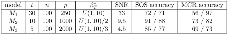
We consider three models with number of potential predictors p exceeding number of ob-servations n. The first model M1 was analyzed in Zhang (2013). Beside it we introduce
two models M2 and M3 which seem to fit even more to the sparse high-dimensional
sce-nario t n p and are described in Table 1, columns 1−4. Observe that sparseness
of the model measured by ratio p/t increases from 8.3 for M1 to 100 for M2 and to 400
for M3. Corresponding ratios p/n are 2.5, 10 and 20, respectively. Note also that the
as-sumptions of either Corollary 2 or Theorem 3 are not satisfied for M1 as 4t > n, whereas two remaining models satisfy 10t ≤ n. In all simulations the n×p matrix of experiment
X with iid standard normal entries is generated and then its columns are normalized to have `2-norm equal to √n. A noise level is specified by σ = 1. For each replication of the true model, elements ofβT∗ are independently generated from uniform distribution with parameters given in the column 5 of Table 1. Such layout resulted in signal to noise ra-tio SN R=||XTβT∗||/pE||ε||2 =||XTβ∗
T||/
√
model t n p βT∗ SNR SOS accuracy MCR accuracy
M1 30 100 250 U(1,10) 33 72 / 71 56 / 97
M2 10 100 1000 U(1,10)/2 9.5 91 / 88 73 / 82
M3 5 100 2000 U(1,10)/3 4.5 85 / 77 69 / 73
Table 1: Summary of the simulations (details explained in the text).
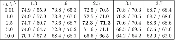
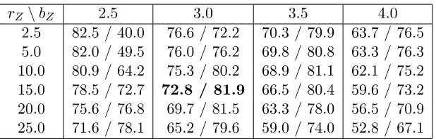
All computations have been performed using open source software R (see supplemental material athttp://www.mimuw.edu.pl/~pokar/Publications/) using two frequently used Lasso implementations: lars (Efron et al., 2004) and glmnet (Friedman et al., 2010). Preliminary experiments indicated that using lars yields higher selection accuracies for SOS as well as for MCR than when using glmnet; even on grids of order 105 the gain in accuracy was around 10%. Moreover, for such dense gridsglmnetwas considerably slower. Thus in main numerical experimentslars has been used. We established that accuracy of SOS for all models is the highest when r ≈20 and thus the value ofr is fixed at 20. The MCR procedure is implemented via the Lasso and LS as described in Section 5.1. Similarly to Zhang (2013) we fixed number of iterations l= 8 for MCR. Thus compared algorithms have mutually corresponding parameters (rL, b) and (rZ, bZ). As in Zhang (2013) we found
optimal grid parameters for which selection accuracy is the highest one. In particular we confirmed high selection accuracy for the best parameters shown in Table 1 in Zhang (2013). Namely, the highest selection accuracy of MCR reported there is 93% for penalty and the threshold both equal 0.94 whereas we found selection accuracy 95% for both these parameters equal to 5. The difference is minor taking into account that the original penalty in Zhang (2013) corresponds in our implementation to 2rZ/
√
n=rZ/5.
As a measure of performance of both algorithms we present in columns 7−8 of Table 1 a percent of correct screening and percent of correct selection separated by the slash that is 100×Pˆ(T ⊆S) / 100×Pˆ( ˆT = T). In simulations for the SOS algorithm, we used as a screening set S = S0 = {j : |θˆj| > b}, since a double-pass screening S1 does not lead
to significant improvement of selection accuracy. Similarly, for MCR we considered as a screening set S ={j : |θjˆ| > bZ} after the first iteration of the algorithm. Knowledge of both screening and selection errors allows us to estimate errors pertaining to ordering and greedy selection for SOS as well as advantage of MCR over the thresholded Lasso. Note that algorithms behave differently in that whereas for MCR probability of correct selection is larger than that of screening after the first iteration, the opposite is true for SOS. Both measures for all grid parameters are reported in Appendix A.4.
All results are based on N = 5000 replicates as for estimation a success probability
π ≈ 0.75 (corresponding crudely to our selection accuracies) in N Bernoulli experiments with prescribed error η = 0.01 and confidence level 1−γ = 0.9, we need N ≈ π(1−
8.2 Conclusions from the Experiments
Computing time of both SOS and MCR is dominated by calls to the lars function which
is used to compute the Lasso, and as MCR uses l = 8 calls of this function and SOS only one, so MCR is around eight time slower than SOS.
For modelM1, MCR is substantially more precise then SOS in selecting the true subset of variables: 97% versus 71%. Recall that the highest accuracy given in Zhang (2013) is 93%. The SOS selection error is mostly due to the screening error of the Lasso as in the case of relatively large number of true predictors compared ton, the Lasso finds it difficult to filtering in all of them.
For models M2 and M3, SOS is more precise than MCR by approximately 5%. We
note that optimal grid penalty rL for SOS and MCR coincide whereas the threshold b is
approximately twice as large for MCR as for SOS. As the results for SOS are better in these cases it turns out that thresholding the Lasso, ranking the remaining estimators and optimizing GIC in the nested family is superior to MCR iterations performed on the same initial Lasso estimator.
In conclusion, if we expect large number of genuine predictors compared to sample size, MCR is preferable, but for the sparse high-dimensional scenario SOS may be faster and more accurate.
For practical model selection we recommend the following easily achievable strategy. After performing the Lasso, we look at the paths of parameters and choose only those whose magnitude is substantially larger than others. This yields screening set S on which LS is computed, and then screened regressors are ordered according to their |t| statistics from the fit. Finally we look for an ’elbow’ of RJ in the nested family of the models
J ∈ {∅,{j1},{j1, j2}, . . . , S} which determines a cut-off point.
9. Concluding Remarks
We introduce the three-step SOS algorithm for a linear model selection. The most compu-tationally demanding part of the method is screening of predictors by the Lasso. Ordering and greedy GIC could be computed using only two QR decompositions of X0S1. In the
paper we give non-asymptotic upper bounds on error probabilities of each step of SOS in terms of the Lasso and GIC penalties (Theorem 1). As corollaries we obtain selection consistency for different (n, p) scenarios under conditions which are needed for screening consistency of the Lasso (Corollaries 1-2). The SOS algorithm is an improvement of the new version of the thresholded Lasso (Zhou, 2009, 2010) and turns out to be competitive for MCR, the latest quasiconvex penalized LS (Zhang, 2010b, 2013). The condition on cor-relation of predictors assumed there seems to be stronger than ours, whereas the beta-min condition may be weaker (compare discussion of Corollary 2 and Theorem 3). Theoretical comparison of SOS and MCR, in general, requires comparingλ3tand κ2(T,3) and remains
It is worth noticing that all results are proved for general form of the Lasso defined in (6), which encompasses two versions of the estimator: algorithm used in practice as well as its formal version.
Acknowledgments
We appreciate comments of two referees which greatly contributed to improving of the original manuscript.
Appendix A: Proofs and Supplemental Tables.
In the Appendix we provide all proofs and supplemental tables for numerical experiments.
A.1 Proofs for Section 3.
Proof of Proposition 1. We have
2σ2KL( ˜βT∗||βJ˜ ) = 2σ2Eβ˜∗
T
||y−X˜Jβ˜J||2− ||y−X˜Tβ˜T∗||2
2σ2
!
=||XT˜ β˜T∗ −XJ˜ βJ˜ ||2.
The last expression is symmetric with respect to ˜βT∗ and ˜βJ, thusKL( ˜β∗T||β˜J) =KL( ˜βJ||β˜T∗)
and the second equality in (i) follows. For the proof of the first equality in (i) observe that
δ(T||J) = minβ˜J||X˜Tβ˜T∗ −X˜Jβ˜J||2. The equality in (ii) follows from (10), the inequality
there follows from Rayleigh-Ritz theorem.
Proof of Proposition 3. We can assume that c≥ 1. Consider a model J and a vector
ν such that J ⊇ supp(ν) and |J| = (bcc+ 1)s and κ2(bcc+ 1)s,0) = νTΣν/νTν. Sort coordinates ofνin nonincreasing order|νj1| ≥ |νj2|. . .≥ |νj(bcc+1)s|and letJ0={j1, . . . , js}. Then we have |J0|=s,|νJ¯0| ≤ bcc|νJ0| ≤c|νJ0|and (bcc+ 1)ν
T
J0νJ0 ≥ν
Tν. Thus
κ2(s, c)≤ ν
TΣν
νT J0νJ0
≤(bcc+ 1)ν
TΣν
νTν = (bcc+ 1)κ
2((bcc+ 1)s,0)
and the conclusion follows.
Proof of Proposition 4. Assume by contradiction that there are two different true mod-els T1, T2 such that Ti = supp(βi) = supp(θi) for some different βi = Dθi, i = 1,2 and µ0 = X0θ1 = X0θ2. It is enough to prove that assumptions imply γ(T1,1)γ(T2,1) = 0, where γ(J, c) = inf{||X0θJ −X0θJ¯||,|θJ|= 1,|θJ¯| ≤c} as in view of (13) and Schwarz
in-equalityκ(J, c)/p|J| ≤γ(J, c). Define a vectorθwith support equal toT1∪T2in such a way
thatθT1∩T2 =θT1∩T2,1−θT1∩T2,2,θT1\T2 =θT1\T2,1 andθT2\T1 =θT2\T1,2. As assumptions on T1 andT2 are symmetric we may assume that|θT1\T2| ≥ |θT2\T1|and letθ
o=θ/|θ
T1|. Then
|θo
T1|= 1 and|θ o
¯ T1|=|θ
o
T2\T1| ≤1. Moreover, Xθ o
T1 =Xθ o
¯
T1 which yields γ(T1,1) = 0. Proof of Proposition 5. To prove (i) observe that (11) and (14) imply for j∈T
For (ii) we have
κ2(t,3)/4 ≤ κ2(4t,0) = min
J:|J|≤4tλmin(ΣJ)≤J:J⊇minT ,|J|≤4tλmin(ΣJ)
= min
J:J+T ,|J∪T|≤4t
λmin(ΣJ∪T)≤θmin∗−2 min J:J+T,|J∪T|≤4t
δ(T||J)
≤ θ∗−min2 min
j∈T ,J⊇T ,|J|≤4tδ(T||J\ {j}) =θ ∗−2
minδ(T,4t),
where the first inequality follows from the Proposition 3 and the third from (11).
A.2 Proofs for Section 6.
We now proceed to prove Theorem 4 and its corollaries. The following modified version of Lemma 1 in Bunea et al. (2007) holds.
Lemma 1 (i) We have on A for an arbitrary β ∈Rp and J ={j:βj 6= 0}
||µ0−µβˆ||2+rL|∆| ≤ ||µ0−µβ||2+ 4rL|∆J|. (33)
(ii) Moreover, we have
||µ0−µβˆ||2 ≤ ||µ0−µβ||2+ 3rL|∆J|. (34) Proof. It follows from (6) that
||H0(ε+µ−Xβˆ)||2+ 2rL|Dβˆ| ≤ ||H0(ε+µ−Xβ)||2+ 2rL|Dβ|.
Equivalently, asH0 is symmetric and idempotent, we get
||H0(µ−Xβˆ)||2≤ ||H0(µ−Xβ)||2+ 2εTH0X( ˆβ−β) + 2rL(|Dβ| − |Dβˆ|).
Thus we obtainthe basic inequality
||µ0−µˆβ||2 ≤ ||µ0−µβ||2+ 2εTX0(ˆθ−θ) + 2rL(|θ| − |θˆ|).
OnA we have |2εTX0(ˆθ−θ)| ≤2 maxj|xT0jε||θˆ−θ| ≤rL|θˆ−θ|and whence on this set
||µ0−µβˆ||2+rL|θˆ−θ| ≤ ||µ0−µβ||2+ 2rL(|θˆ−θ|+|θ| − |θˆ|).
Note that forj6∈J |θˆj−θj|+|θj| − |θˆj|= 0 and thus
||µ0−µβˆ||2+rL|θˆ−θ| ≤ ||µ0−µβ||2+ 2rL(|θˆJ −θJ|+|θJ| − |θˆJ|).
Thus (i) follows from triangle inequality and (ii) from (i) in view of |θˆJ−θJ| ≤ |θˆ−θ|.
inequality ||µ0−µβˆ|| ≤ ||µ0−µβ|| holds. When (b) is satisfied we have |∆J¯| ≤3|∆J| and
it follows from the definition ofκ that κ2||∆J||2≤ ||X0∆||2 =||µβˆ−µβ||2 and thus
||∆J|| ≤ ||µβˆ−µβ||κ−1. (35)
Using (35) and Jensen inequality we get
|∆J| ≤ |J|1/2||µβˆ−µβ||κ−1. (36)
It follows now from (34), (36) and triangle inequality that
||µ0−µβˆ||2≤ ||µ0−µβ||2+ 3rL|J|1/2κ−1(||µ0−µβˆ||+||µ0−µβ||)
and whence
(||µ0+µβˆ||+||µ0−µβ||)(||µ0−µβˆ|| − ||µ0−µβ||)≤3rL|J|1/2κ−1(||µ0−µβˆ||+||µ0−µβ||)
from which the conclusion follows.
Proof of (ii). Define m=||µ0−µβ||, ˆm=||µ0−µβˆ||and c= 2rL|J|1/2κ−1. Using (33),
(36) which holds provided |∆| ≤4|∆J|, and triangle inequality we get
ˆ
m2+rL|∆| ≤m2+ 2c( ˆm+m)≤2m2+c2+ ˆm2+c2,
from which the desired bound follows.
Proof of Corollary 8. The proof follows from inequality (35), (36) and the second in-equality in Corollary 7.
A.3 Proofs for Section 4.
The next lemma states bounds on upper tail ofχ2k distribution
Lemma 2 LetWkdenote variable havingχ2kdistribution.(i) (Gordon, 1941 and Mill, 1926)
We have fork= 1 and x >0
wxklxk≤P(Wk ≥x)≤wxk, (37)
where wxk=e−x/2(x2)k/2−1Γ−1(k2) and lxk= x−xk+2.
(ii) (Inglot and Ledwina, 2006) Let k >1 andx > k−2. Then
wxk ≤P(Wk≥x)≤wxklxk. (38)
Proof. We provide the unified reasoning for both cases. For x >0 and k∈Zlet Ik(x) = R∞
x t
(k/2)−1e−t/2dt. Integration by parts yields
It is easy to see that the following inequalities hold for x >0 andk∈Z
0≤Ik−2(x)≤Ik(x)/x. (40)
We treat casesk= 1 andk >1 separately, ask= 1 is the only integer for which the second term on the RHS of (39) is negative. Dividing both sides of (39) by 2k/2Γ(k/2), noting that
the LHS is thenP(Wk≥x) and using (40) we have for k= 1 and x >0
P(Wk ≥x)≤e−x/2 x
2
−1/2
Γ−11 2
and
P(Wk≥x)≥e−x/2 x
2
−1/2
Γ−11 2
1− 1
1 +x
,
which proves (37). Analogously fork= 2,3, . . . we obtain from (39) inequalities proved by Inglot and Ledwina (2006)
P(Wk≥x)≤e−x/2 x
2
k/2−1
Γ−1k 2
1 + k−2
x−k+ 2
forx > k−2, and forx >0
P(Wk≥x)≥e−x/2 x
2
k/2−1
Γ−1
k
2
,
which proves (38).
Now we state the main lemma from which Theorems 1 and 2 follow. Let us recall that
c1 = (3 + 6√2)−1 and c2 = (6 + 4√2)−1. Define To
n = Tn\ {T} and observe that for OS
algorithm we haveP(S16∈ Tn) = 0 and as p≥t+ 1, Tn=Tno ={F}, so|Tno|= 1.
Lemma 3 (T1) If rL2 ≤b2/36≤c21t−1κ4θmin∗2 , then
P(S1 6∈ Tn)≤pexp
− r
2 L
8σ2
πr2L
8σ2 −1/2
.
(T2) Ifs≤n, then
P(S1 ∈ Tn,Oˆ 6∈OS1)≤
3 2|T
o
n|t(s−t) exp
−c2δs
σ2 πc2δs σ2 −1/2 .
(T3) If for somea∈(0,1) r ≤at−1δt, then
P(S1 ∈ Tn,Oˆ ∈OS1,|Tˆ|< t)≤ t
2exp
− (1−a)
2δ t
8σ2
π(1−a)2δt
8σ2
−1/2 .
(T4) Assume that r/σ2≥2 and (r/σ2)−log(r/σ2)≥2 logp. Then
P(S1∈ Tn,Oˆ ∈OS1,|Tˆ|> t)≤(p−t)(s−t) exp
− r
2σ2
πr
2σ2 −1/2
Proof. Observe that we may assume that t > 0 in proofs of (T2)−(T3) as for t = 0 probabilities appearing in those parts are 0 and the conclusions are trivially satisfied.
Proof of (T1). It follows from (29) or equivalently from Lemma 2 that it is enough to prove that {S1∈ Tn} ⊇ A that is that onAwe have
T ⊆S1 and |S1| ≤t+b
√
tκ−2c. (41)
For parametric models µβ = µ0 and from (33) we have |∆| ≤ 4|∆T| or equivalently
4|∆T¯| ≤3|∆|, which together with the first part of (32) yields
|∆T¯| ≤6rLtκ−2. (42)
From the assumption 6rL ≤ b and (42) we obtain |S0 \T| < |∆T¯|/b ≤ tκ−2, |S0| < t(1 +κ−2) and B < bpt(1 +κ−2). Using this and the first part of Corollary 8 we have
||∆T||+B < θmin∗ or
||∆T||2<(θ∗min−B)2.
Indeed, from Corollary 8, the fact thatκ≤1 and the assumption of the lemma, respectively, we have
||∆T||+B <3rLt1/2κ−2+b p
t(1 +κ−2)≤0.5bt1/2κ−2(1 + 2√κ4+κ2)
≤0.5(1 + 2√2)bt1/2κ−2 = (6c1)−1bt1/2κ−2 ≤θmin∗ .
Evidently, |T \S1|(θ∗min −B)2 ≤ ||∆T||2 < (θmin∗ −B)2 and thus we have T ⊆ S1 on
A. But S1 ⊆ S0, hence |S0| ≥ t and B ≥ bt1/2. Thus using (42) again, we have
|S1\T|<|∆T¯|/B≤t1/2κ−2.Hence |S1\T| ≤ bt1/2κ−2cand we obtain (41).
Proof of (T2). Let forJ1 ∈ Sn\ Tnand J2∈ TnWJ1J2 =ε T( ˜H
J1−H˜J1∩J2)ε,σ 2W
J2J1 = εT( ˜HJ2 −HJ˜ 1∩J2)ε and σZJ1 = ˜β
∗T
T X˜TT(I −HJ˜ 1)ε/ p
δJ1, where δJ1 =δ(T kJ1). Then we
have that WJ1J2 ∼ χ 2
d, where d≤ |J1 \J2|, WJ2J1 ≥ 0 and ZJ1 ∼N(0,1). We will use a
popular decomposition of a difference between sums of squared residuals
RJ1−RJ2 = β˜ ∗T
T X˜TT(I−HJ˜ 1) ˜XTβ˜ ∗ T + 2 ˜β
∗T
T X˜TT(I−HJ˜ 1)ε
+ εT(I −H˜J1)ε−ε
T(I−H˜ J2)ε
= δJ1+ 2 p
δJ1σZJ1−σ 2W
J1J2 +σ 2W
J2J1
≥ δJ1
1 +2σZJ1 p
δJ1
−σ
2W J1J2 δJ1
.
For fixed S∈ To
n let ¯j=S\ {j}. Then we have from (9)
{S1 ∈ Tno,Oˆ 6∈OS1} ⊆ [
S∈To n
[
j1∈T [
j2∈S\T
{R¯j1 ≤R¯j2}
⊆ [
S∈To n
[
j1∈T [
j2∈S\T n
−2σZ¯j1 p
δ¯j1 +
σ2W¯j1¯j2 δ¯j1 ≥1
whereZ¯j1 ∼N(0,1) andW¯j1¯j2 ∼χ 2
d, withd≤1. Thus it follows that forW =Z2 denoting
r.v. with χ21 distribution, we get
P(S1 ∈ Tno,Oˆ6∈OS1) ≤ X
S∈To n
X
j1∈T X
j2∈S\T
P−2σZ¯j1 p
δ¯j1 +
σ2W¯j1¯j2 δ¯j1 ≥1
≤ X
S∈To n
X
j1∈T X
j2∈S\T
P
−2σZ¯j1 p
δ¯j1 ≥c
+P
σ2W¯j 1¯j2
δ¯j1 ≥1−c
≤ |Tno|t(s−t)1 2P
Z2≥ c
2δs
4σ2
+PW ≥ (1−c)δs
σ2
,
wherej1∈T andj2∈S\T are fixed and we usedδ¯j1 ≥δs. Choosingcsuch thatc2/4 = 1−c
that is c= 1−2c2 in view of Lemma 2 we get the desired bound.
Proof of (T3). Reasoning as previously we have for ¯j=T\ {j}
{S1∈ Tn,Oˆ ∈OS1,|Tˆ|< t} ⊆ [
S⊂T
{RS+r|S| ≤RT +r|T|} ⊆ [
j∈T
{R¯j ≤RT +rt}.
Thus in view of Lemma 2 and the assumption rt < aδt we obtain
P(S1 ∈ Tn,Oˆ∈OS1,|Tˆ|< t) ≤ X
j∈T
P(R¯j ≤RT +rt)
≤ X
j∈T
P−2σZ¯j ≥qδ¯j1−rt
δ¯j
≤ tP
−2σZ ≥pδt
1−rt
δt
= t
2P
W ≥ 1 4σ2δt
1−rt
δt 2
≤ t
2exp
−(1−a)
2δt
8σ2
π(1−a)2δt
8σ2
−1/2 .
Proof of (T4). Observe first that for m >0
P(S1 ∈ Tn,Oˆ ∈OS1,|Tˆ|=t+m)
≤P(RT∪{j1,...,jm}+ (t+m)r ≤RT +tr for somej1, . . . , jm∈F\T) ≤
p−t
m
P(σ2Wm≥mr)≤
(p−t)m
m! P(σ
2W
m ≥mr) =Bm,
whereWm ∼χ2m. This follows since for any fixedJ =T∪ {j1, . . . , jm}we haveRT −RJ ∼ σ2χ2
d, whered≤m andWd≤Wm in stochastic order. We will show that under conditions
given in (T4)Bm ≥Bm+1 for any m= 1,2, . . . thus yielding
P(S1∈ Tn,Oˆ ∈OS1,|Tˆ| ≥t+m)≤(s−t−m+ 1)Bm,
which for m= 1 coincides with the desired inequality. Let Qm =Bm/Bm+1, ¯r =r/σ2 and
observe that for m >1 we have in view of (38) (note that mr¯≥m−2 as ¯r≥2)
Qm≥ m+ 1
p e ¯ r/2 m
m+ 1
m/2−1 1
(m+ 1)¯r/21/2
Γ((m+ 1)/2) Γ(m/2)
Using the inequality for gamma functions (cf. formula 2.2 in Laforgia, 1984)
Γ
m+ 1
2 . Γ m 2
≥m−1/2 2
1/2
we have that
Qm≥exp nr¯
2 −
1
2log ¯r−logp
o
f1(m,r¯),
where
f1(m,r¯) =
m
m+ 1
m/2−1
(m+ 1)1/221/2m−1/2 2
1/2(m+ 1)¯r−m+ 1
(m+ 1)¯r .
Thus in order to show that Qm ≥ 1 for m > 1 in view of assumptions it is enough to show thatf1(m,r¯)>1. Asf(m,·) is increasing, it suffices to check that f1(m,2)>1. Let f2(m) = (mm+1−1/2)(m−1)/2(m+32 ). We havef1(m,2)> f2(m) and f2(2)>1 thus it is enough to show thatf2 is increasing. Let
f3(m) = log(2f2(m)) = m−1
2 log
m−1/2
m+ 1 + log(m+ 3).
We have that
f30(m) = 1 2log
m−1/2
m+ 1 +
m−1 2
m+ 1 (m−1/2)
3 2(m+ 1)2 +
1
m+ 3
≥ 1
2
−3
−3 + 2(m+ 1) +
3(m−1)
4(m−1/2)(m+ 1)+ 1
m+ 3,
where the last inequality follows from log(1 +x)> x/(1 +x) forx >−1. As 1/(m+ 3)≥ 3/(−6 + 2(m+ 1)) it follows thatf30 >0 which implies that f3 and thus f2 is increasing.
Proof of Theorem 1. The result readily follows from Lemma 3. For (T1) we observe that
− r
2 L
8σ2 + logp≤ −
(1−a)r2L
8σ2
is equivalent to 8σ2a−1logp ≤ rL2. Similar reasoning yields (T4). Consider derivation of (T2). From the bound
|Tno|=|Tn| −1 = s−t X
k=1
p−t k
≤(p−t) +. . .+(p−t)
s−t
(s−t)! ≤
(p−t)s−t (s−t)! (s−t)
it follows that |To
n|t(s−t)≤(p−t)s−tt(s−t)≤ps−tt(s−t).Thus the bound in (T2) will
follow from −c2δn/σ2+ (s−t) logp+ log(s−t) + logt≤ −c2(1−a)δs/σ2 which is implied by (s−t+ 2) logp≤c2aδs/σ2. For (T3) we observe that
−(1−a)
2δt
8σ2 + logt≤ −
(1−a)3δt
8σ2
Proof of Corollary 1. We proceed by showing that assumptions (i) and (ii) imply all assumptions of Theorem 1. We first note that (i) with the assumption rL2 = 4r is stronger than the assumption in Theorem 1 (T1). Next, observe that condition
4a−1σ2logp≤(4c2/3)t−1/2κ2δs (43)
is stronger than the assumption in Theorem 1 (T2). Indeed, asκ≤1≤twe have
s−t+ 2 =bt1/2κ−2c+ 2≤t1/2κ−2+ 2≤3t1/2κ−2.
Obviously, left inequalities in (i) and (ii) imply (43). Moreover, the assumption of Theorem 1 (T4) is satisfied. Furthermore, from the first κ−δ inequality (15) and assumption a∈ (0,1−c1) we obtain that (i) is stronger than both conditions in Theorem 1 (T3).
In order to justify the conclusion, in view of the fact thate−(1−a)x(πx)−1/2 is decreasing function ofx >0, it is enough to show that the expressions in the exponents of the bounds (19) and (20) are larger than r/(2σ2) that is a value in the exponents of the bounds (18) and (21) . In the case of (19) the condition is equivalent to r ≤2c2δs, which is implied by
(ii). In the case of (20) the ensuing inequality is implied by r ≤((1−a)2/4)κ2θ∗min2 which in turn is implied by (i) as a∈(0,1−c1).
Proof of Theorem 2. Let us recall that for OS algorithm we have P(S1 6∈ Tn) = 0 and
|To
n|= 1, so the results follow from Lemma 3 analogously to Theorem 1.
Proof of Corollary 3. We proceed as in the proof of Corollary 1. The following condition
4a−1σ2logp≤2c2δs. (44)
is stronger than the assumption in Theorem 2. The assumption imply (44) and the assump-tion of (T4). Furthermore, from the firstκ−δ inequality (15) and assumption a∈(0,2c2) we obtain that the assumption is stronger than both conditions in (T3).
Next we show that the powers in the exponents of the bounds (19) and (20) are larger thanr/(2σ2). In the case of (19) the condition is equivalent tor ≤2c2δswhich is implied by the assumption. In the case of (20) the ensuing inequality is implied byr≤((1−a)2/4)δt,
which is implied byr≤at−1δ
tbecause fora∈(0,1) a conditiona≤(1−a)2/4 is equivalent
toa∈(0,2c2).
A.4 Proof for Section 5.
Proof of Theorem 3. Let vjT = xTj(I −HT) for j 6∈ T and 0 otherwise and uTj =
eTj(XTTXT)−1XTT forj∈T and 0 otherwise, whereej is the unit vector having 1 as thejth
coordinate. Let
A=
n
∀j∈F |vTjε|< 2rZ
7 ,|u
T jε|<
2rZ
7λt o
.
Using the left part of the assumption (ii), we observe that the following statement, which is equivalent of Lemma 3 in Zhang (2013) in the case of Gaussian errors, holds
P(Ac)≤exp
−c3(1−a)r2 Z σ2
c3πr2 Z σ2
−1/2
Then the proof of Theorem 3 follows the lines of the original proof in Zhang (2013), but just before the end we simplify the condition l > l0+ 1, noting that
l0 =
lnt
2 ln(λ1.5t+sbZ/(6rZ))
≤ lnt
2 ln(1.5) <1.24 lnt.
In order to prove (45) observe that for j 6∈ T var(vjTε) = σ2xTj(I −HT)xj ≤ σ2 and
Wj = (vjTε)2/var(vTjε)∼χ21. Thus using Mill’s inequality (37) we have
P
|vTjε| ≥ 2rZ 7
≤P
Wj ≥ 2c3r
2 Z σ2
≤exp
−c3r2 Z σ2
c3πr2 Z σ2
−1/2
. (46)
Using the same reasoning for j ∈ T with var(uTjε) = σ2eTj(XTTXT)−1ej ≤ σ2λ−t1 and ˜
Wj = (uTjε)2/var(uTjε)∼χ21, we have
P
|uTjε| ≥ 2rL 7√λt
≤P
˜
Wj ≥ 2c3r
2 Z σ2
≤exp
−c3r2 Z σ2
c3πr2 Z σ2
−1/2
. (47)
From (46) and (47) we obtain with c= 2c3rZ2/σ2 P(Ac)≤X
j∈T
P( ˜Wj ≥c) + X
j6∈T
P(Wj ≥c)≤pexp
−c3r2 Z σ2
c3πr2 Z σ2
−1/2 .
Finally, we observe that inequality
−c3r2Z/σ2+ logp≤ −(1−a)c3r2Z/σ2
A.4 Tables for Section 8.
rL\b 1.3 1.9 2.5 3.1 3.7
0.01 74.9 / 55.9 73.8 / 65.3 72.5 / 70.5 70.8 / 70.3 68.7 / 68.4
1.0 74.9 / 57.9 73.8 / 67.0 72.5 / 71.0 70.8 / 70.5 68.7 / 68.6
2.5 74.7 / 60.7 73.6 / 68.7 72.3 / 71.3 70.6 / 70.4 68.6 / 68.6
5.0 74.0 / 64.7 72.8 / 70.2 71.6 / 71.1 69.5 / 69.5 67.6 / 67.6
10.0 70.1 / 67.2 68.4 / 68.1 66.5 / 66.5 64.2 / 64.2 62.0 / 62.0
Table 2: Screening / selection accuracy of SOS forM1, r= 20.
rL\b 0.6 0.9 1.2 1.5 1.8
5.0 95.7 / 74.0 94.2 / 78.8 92.6 / 83.9 90.6 / 86.0 88.5 / 85.7
10.0 95.5 / 78.1 94.2 / 83.4 92.5 / 86.7 90.5 / 87.1 87.8 / 85.4
15.0 94.7 / 82.0 93.1 / 85.9 91.3 / 87.5 89.1 / 86.6 86.1 / 84.2
20.0 93.1 / 85.1 91.2 / 86.7 89.1 / 86.4 86.1 / 84.2 83.6 / 82.2
30.0 87.6 / 84.7 85.1 / 83.1 82.2 / 80.9 78.4 / 77.4 75.2 / 74.4
Table 3: Screening / selection accuracy of SOS forM2, r= 20.
rL\b 0.4 0.8 1.2 1.6 2.0
2.5 93.0 / 69.4 90.1 / 70.0 86.4 / 74.4 82.4 / 75.5 78.3 / 74.3
5.0 93.0 / 69.7 90.1 / 71.6 86.4 / 75.3 82.4 / 76.0 78.2 / 74.7
10.0 92.5 / 70.0 89.4 / 72.8 85.6 / 76.3 81.9 / 76.2 77.8 / 74.8
15.0 91.7 / 71.2 88.6 / 74.8 84.9 / 76.9 80.4 / 76.0 76.5 / 74.2
25.0 88.7 / 74.8 84.8 / 76.8 80.5 / 76.0 76.0 / 73.7 72.2 / 71.0
35.0 82.0 / 76.1 77.4 / 74.2 73.2 / 71.6 68.7 / 67.9 64.5 / 64.2
Table 4: Screening / selection accuracy of SOS forM3, r= 20.
rZ\bZ 4.0 5.0 6.0 7.0
0.5 67.5 / 63.0 63.3 / 90.9 57.8 / 95.6 50.7 / 94.2
2.5 67.5 / 75.0 63.3 / 94.1 57.8 / 96.3 50.7 / 94.6
5.0 66.2 / 84.5 61.9 / 95.4 56.0 / 96.9 48.7 / 94.8
10.0 60.8 / 90.4 55.2 / 96.5 49.0 / 96.9 41.8 / 94.2
20.0 43.8 / 93.9 37.3 / 96.8 31.4 / 96.0 25.6 / 90.0
30.0 28.0 / 94.2 23.0 / 95.3 18.9 / 90.0 15.1 / 78.8