Towards Ultrahigh Dimensional Feature Selection
for Big Data
Mingkui Tan [email protected]
School of Computer Engineering Nanyang Technological University
Blk N4, #B1a-02, Nanyang Avenue 639798, Singapore
Ivor W. Tsang [email protected]
Center for Quantum Computation&Intelligent Systems University of Technology Sydney, Sydney P.O. Box 123, Broadway, NSW 2007 Sydney, Australia
Li Wang [email protected]
Department of Mathematics, University of California San Diego 9500 Gilman Drive La Jolla, CA 92093, USA
Editor:Sathiya Keerthi
Abstract
In this paper, we present a new adaptive feature scaling scheme for ultrahigh-dimensional feature selection onBig Data, and then reformulate it as a convex semi-infinite programming (SIP) problem. To address the SIP, we propose an efficient feature generating paradigm. Different from traditional gradient-based approaches that conduct optimization on all in-put features, the proposed paradigm iteratively activates a group of features, and solves a sequence of multiple kernel learning (MKL) subproblems. To further speed up the training, we propose to solve the MKL subproblems in their primal forms through a modified accel-erated proximal gradient approach. Due to such optimization scheme, some efficient cache techniques are also developed. The feature generating paradigm is guaranteed to converge globally under mild conditions, and can achieve lower feature selection bias. Moreover, the proposed method can tackle two challenging tasks in feature selection: 1) group-based feature selection with complex structures, and 2) nonlinear feature selection with explicit feature mappings. Comprehensive experiments on a wide range of synthetic and real-world data sets of tens of million data points with O(1014) features demonstrate the
competi-tive performance of the proposed method over state-of-the-art feature selection methods in terms of generalization performance and training efficiency.
Keywords: big data, ultrahigh dimensionality, feature selection, nonlinear feature selec-tion, multiple kernel learning, feature generation
1. Introduction
requirements and high computational cost in training, but also deteriorates the general-ization ability because of the “curse of dimensionality” issue (Duda et al., 2000.; Guyon and Elisseeff, 2003; Zhang and Lee, 2006; Dasgupta et al., 2007; Blum et al., 2007). For-tunately, for many data sets with ultrahigh dimensions, most of the features are irrelevant to the output. Accordingly, dropping the irrelevant features and selecting the most rele-vant features can vastly improve the generalization performance (Ng, 1998). Moreover, in many applications such as bioinformatics (Guyon and Elisseeff, 2003), a small number of features (genes) are required to interpret the results for further biological analysis. Finally, for ultrahigh-dimensional problems, a sparse classifier is important for faster predictions.
Ultrahigh dimensional data also widely appear in many nonlinear machine learning tasks. For example, to tackle the intrinsic nonlinearity of data, researchers proposed to achieve fast training and prediction through linear techniques using explicit feature map-pings (Chang et al., 2010; Maji and Berg, 2009). However, most of the explicit feature mappings will dramatically expand the data dimensionality. For instance, the commonly used 2-degree polynomial kernel feature mapping has a dimensionality of O(m2), where m
denotes the number of input features (Chang et al., 2010). Even with a medium m, the dimensionality of the induced feature space is very huge. Other typical feature mappings include the spectrum-based feature mapping for string kernel (Sonnenburg et al., 2007; Sculley et al., 2006), histogram intersection kernel feature expansion (Wu, 2012), and so on. Numerous feature selection methods have been proposed for classification tasks in the last decades (Guyon et al., 2002; Chapelle and Keerthi, 2008). In general, existing feature selection methods can be classified into two categories, namely filter methods and wrapper methods (Kohavi and John, 1997; Ng, 1998; Guyon et al., 2002). Filter methods, such as the signal-to-noise ratio method (Golub et al., 1999) and the spectral feature filtering (Zhao and Liu, 2007), own the advantages of low computational cost, but they are incapable of finding an optimal feature subset w.r.t. a predictive model of interest. On the contrary, by incorporating the inductive learning rules, wrapper methods can select more relevant features (Xu et al., 2009a; Guyon and Elisseeff, 2003). However, in general, the wrapper methods are more computationally expensive than the filter methods. Accordingly, how to scale the wrapper methods to big data is an urgent and challenging issue, and is also a major focus of this paper.
expen-sive especially for high dimensional problems. Xu et al. proposed another non-monotonic feature selection method, namely NMMKL (Xu et al., 2009a). Unfortunately, NMMKL is computationally infeasible for high dimensional problems since it involves a QCQP problem with many quadratic constraints.
Focusing on the logistic loss, recently, some researchers proposed to select features using greedy strategies (Tewari et al., 2011; Lozano et al., 2011), which iteratively include one feature into a feature subset. For example, Lozano et al. (2011) proposed a group orthogonal matching pursuit. Tewari et al. (2011) further introduced a general greedy scheme to solve more general sparsity constrained problems. Although promising performance has been observed, the greedy methods have several drawbacks. For example, since only one feature is involved in each iteration, these greedy methods are very expensive when there are a large number of features to be selected. More critically, due to the absence of appropriate regularizer in the objective function, the over-fitting problem may happen, which may deteriorate the generalization performance (Lozano et al., 2011; Tewari et al., 2011).
Given a set of labeled patterns{xi, yi}ni=1, wherexi ∈Rmis an instance withmfeatures, and yi ∈ {±1} is the output label. To avoid the over-fitting problem or induce sparsity,
people usually introduce some regularizers to the loss function. For instance, to select features that contribute the most to the margin, we can learn a sparse decision function
d(x) =w0xby solving:
min
w kwk0+C
n
X
i=1
l(−yiw0xi),
wherel(·) is a convex loss function,w∈Rm is the weight vector,kwk0denotes the`0-norm
that counts the number of non-zeros inw, andC >0 is a regularization parameter. Unfortu-nately, this problem is NP-hard due to the`0-norm regularizer. Therefore, many researchers
resort to learning a sparse decision rule through an `1-convex relaxation instead (Bradley and Mangasarian, 1998; Zhu et al., 2003; Fung and Mangasarian, 2004):
min
w kwk1+C
n
X
i=1
l(−yiw0xi), (1)
wherekwk1=Pmj=1|wj|is the`1-norm onw. The`1-regularized problem can be efficiently
solved, and many optimization methods have been proposed to solve this problem, including Newton methods (Fung and Mangasarian, 2004), proximal gradient methods (Yuan et al., 2011), coordinate descent methods (Yuan et al., 2010, 2011), and so on. Interested readers can find more details of these methods in (Yuan et al., 2010, 2011) and references therein. Beside these methods, recently, to address the big data challenge, great attention has been paid on online learning methods and stochastic gradient descent (SGD) methods for dealing with big data challenges (Xiao, 2009; Duchi and Singer, 2009; Langford et al., 2009; Shalev-Shwartz and Zhang, 2013).
However, there are several deficiencies regarding these `1-norm regularized model and existing `1-norm methods. Firstly, since the`1-norm regularization shrinks the regressors,
Pn
i=1l(−yiw0xi) be the empirical loss on the training data, then w∗ is an optimal solution
to (1) if and only if it satisfies the following optimality conditions (Yuan et al., 2010):
∇jL(w∗) =−1/C if w∗j >0, ∇jL(w∗) = 1/C if w∗j <0, −1/C≤ ∇jL(w∗)≤1/C if w∗j = 0.
(2)
According to the above conditions, one can achieve different levels of sparsity by changing the regularization parameter C. On one hand, using a small C, minimizing kwk1 in (1) would favor selecting only a few features. The sparser the solution is, the larger the predic-tive risk (or empirical loss) will be (Lin et al., 2010). In other words, the solution bias will happen (Figueiredo et al., 2007). In an extreme case, where C is chosen to be tiny or even close to zero, none of the features will be selected according to the condition (2), which will lead to a very poor prediction model. On the other hand, using a large C, one can learn an more fitted prediction model to to reduce the empirical loss. However, according to (2), more features will be included. In summary, the sparsity and the unbiased solutions cannot be achieved simultaneously via solving (1) by changing the tradeoff parameterC. A possible solution is to do de-biasing with the selected features using re-training. For example, we can use a large C to train an unbiased model with the selected features (Figueiredo et al., 2007; Zhang, 2010b). However, such de-biasing methods are not efficient.
Secondly, when tackling big data of ultrahigh dimensions, the `1-regularization would
be inefficient or infeasible for most of the existing methods. For example, when the di-mensionality is around 1012, one needs about 1 TB memory to store the weight vector w, which is intractable for existing `1-methods, including online learning methods and SGD
methods (Langford et al., 2009; Shalev-Shwartz and Zhang, 2013). Thirdly, due to the scale variation of w, it is also non-trivial to control the number of features to be selected meanwhile to regulate the decision function.
In the conference version of this paper, an`0-norm sparse SVM model is introduced (Tan
et al., 2010). Its nice optimization scheme has brought significant benefits to several appli-cations, such as image retrieval (Rastegari et al., 2011), multi-label prediction (Gu et al., 2011a), feature selection for multivariate performance measures (Mao and Tsang, 2013), fea-ture selection for logistic regression (Tan et al., 2013), and graph-based feafea-ture selection (Gu et al., 2011b). However, several issues remain to be solved. First of all, the tightness of the convex relation remains unclear. Secondly, the adopted optimization strategy is incapable of dealing with very large-scale problems with many training instances. Thirdly, the pre-sented feature selection strategy was limited to linear features, but in many applications, one indeed needs to tackle nonlinear features that are with complex structures.
Regarding the above issues, in this paper, we propose an adaptive feature scaling (AFS) for feature selection by introducing a continuous feature scaling vector d∈[0,1]m. To en-force the sparsity, we impose an explicit`1-constraint||d||1≤B, where the scalarB
repre-sents the least number of features to be selected. The solution to the resultant optimization problem is non-trivial due to the additional constraint. Fortunately, by transforming it as a convex semi-infinite programming (SIP) problem, an efficient optimization scheme can be developed. In summary, this paper makes the following extensions and improvements.
of performing the optimization on all input features, FGM iteratively infers the most informative features, and then solves a reduced multiple kernel learning (MKL) sub-problem, where each base kernel is defined on a set of features.1
• The proposed optimization scheme mimics the re-training strategy to reduce the fea-ture selection bias with little effort. Specifically, the feafea-ture selection bias can be effectively alleviated by separately controlling the complexity and sparsity of the de-cision function, which is one of the major advantages of the proposed scheme.
• To speed up the training on big data, we propose to solve the primal form of the MKL subproblem by a modified accelerated proximal gradient method. As a result, the memory requirement and computational cost can be significantly reduced. The convergence rate of the modified APG is also provided. Moreover, several cache techniques are proposed to further enhance the efficiency.
• The feature generating paradigm is also extended to group feature selection with com-plex group structures and nonlinear feature selection using explicit feature mappings.
The remainder of this paper is organized as follows. In Section 2, we start by presenting the adaptive feature scalings (AFS) for linear feature selection and group feature selection, and then present the convex SIP reformulations of the resultant optimization problems. Af-ter that, to solve the SIP problems, in Section 3, we propose the feature generating machine (FGM) which includes two core steps, namely the worst-case analysis step and the subprob-lem optimization step. In Section 4, we illustrate the worst-case analysis for a number of learning tasks, including the group feature selection with complex group structures and the nonlinear feature selection with explicit feature mappings. We introduce the subproblem optimization in Section 5 and extend FGM for multiple kernel learning w.r.t. many addi-tive kernels in Section 6. Related studies are presented in Section 7. We conduct empirical studies in Section 8, and conclude this work in Section 9.
2. Feature Selection Through Adaptive Feature Scaling
Throughout the paper, we denote the transpose of vector/matrix by the superscript 0, a vector with all entries equal to one as1∈Rn, and the zero vector as 0∈
Rn. In addition, we denote a data set by X = [x1, ...,xn]0 = [f1, ...,fm], where xi ∈ Rm represents the ith instance andfj ∈Rndenotes the jth feature vector. We use|G|to denote cardinality of an index setGand|v|to denote the absolute value of a real numberv. For simplicity, we denote
vαifvi ≥αi,∀iandvαifvi≤αi,∀i. We also denotekvkpas the`p-norm of a vector
and kvk as the `2-norm of a vector. Given a vector v = [v01, ...,v0p]0, where vi denotes a
sub-vector ofv, we denotekvk2,1=Pip=1kvikas the mixed`1/`2 norm (Bach et al., 2011)
and kvk2 2,1 = (
Pp
i=1kvik)2. Accordingly, we call kvk22,1 as an `22,1 regularizer. Following
Rakotomamonjy et al. (2008), we define xi
0 = 0 ifxi = 0 and ∞ otherwise. Finally,AB
represents the element-wise product between two matricesA and B.
2.1 A New AFS Scheme for Feature Selection
In the standard support vector machines (SVM), one learns a linear decision functiond(x) =
w0x−bby solving the following `2-norm regularized problem:
min w
1 2kwk
2+C
n
X
i=1
l(−yi(w0xi−b)), (3)
where w = [w1, . . . , wm]0 ∈ Rm denotes the weight of the decision hyperplane, b denotes the shift from the origin, C >0 represents the regularization parameter andl(·) denotes a convex loss function. In this paper, we concentrate on two kinds of loss functions, namely the squared hinge loss
l(−yi(w0xi−b)) =
1
2max(1−yi(w
0x
i−b),0)2
and the logistic loss
l(−yi(w0xi−b)) = log(1 + exp(−yi(w0xi−b))).
For simplicity, herein we concentrate the squared hinge loss only.
In (3), the `2-regularizer ||w||2 is used to avoid the over-fitting problem (Hsieh et al.,
2008), which, however, cannot induce sparse solutions. To address this issue, we introduce a feature scaling vectord∈[0,1]m such that we can scale the importance of features.
Specifi-cally, given an instancexi, we impose
√
d= [√d1, . . . ,√dm]0 on its features (Vishwanathan
et al., 2010), resulting in a re-scaled instance
b
xi = (xi
√
d). (4)
In this scaling scheme, the jth feature is selected if and only if dj >0.
Note that, in many real-world applications, one may intend to select a desired number of features with acceptable generalization performance. For example, in the Microarray data analysis, due to expensive bio-diagnosis and limited resources, biologists prefer to select less than 100 genes from hundreds of thousands of genes (Guyon et al., 2002; Golub et al., 1999). To incorporate such prior knowledge, we explicitly impose an`1-norm constraint on d to induce the sparsity:
m
X
j=1
dj =||d||1 ≤B, dj ∈[0,1], j = 1,· · ·, m,
where the integer B represents the least number of features to be selected. Similar feature scaling scheme has been used by many works (e.g., Weston et al., 2000; Chapelle et al., 2002; Grandvalet and Canu, 2002; Rakotomamonjy, 2003; Varma and Babu, 2009; Vishwanathan et al., 2010). However, different from the proposed scaling scheme, in these scaling schemes,
d is not bounded in [0, 1]m. Let D =
d ∈ Rm
Pm
j=1dj ≤B, dj ∈ [0,1], j = 1,· · ·, m be the domain of d, the
proposed AFS can be formulated as the following problem:
min d∈Dwmin,ξ,b
1 2kwk
2 2+
C
2
n
X
i=1
ξi2 (5)
s.t. yi
w0(xi
√ d)−b
where C is a regularization parameter that trades off between the model complexity and the fitness of the decision function, and b/kwk determines the offset of the hyperplane from the origin along the normal vector w. This problem is non-convex w.r.t. w and d
simultaneously, and the compact domainDcontains infinite number of elements. However, for a fixedd, the inner minimization problem w.r.t. wand ξ is a standard SVM problem:
min w,ξ,b 1 2kwk 2 2+ C 2 n X i=1
ξi2 (6)
s.t. yi
w0(xi
√ d)−b
≥1−ξi, i= 1,· · · , n,
which can be solved in its dual form. By introducing the Lagrangian multiplierαi ≥0 to
each constraint yi
w0(xi
√
d)−b≥1−ξi, the Lagrangian function is:
L(w,ξ, b,α) = 1 2kwk 2 2+ C 2 n X i=1 ξi2−
n X i=1 αi yi
w0(xi
√ d)−b
−1 +ξi
. (7)
By setting the derivatives of L(w,ξ, b,α) w.r.t. w,ξ and bto0, respectively, we get
w=
n
X
i=1
αiyi(xi
√
d),α=Cξ, and
n
X
i=1
αiyi= 0. (8)
Substitute these results into (7), and we arrive at the dual form of problem (6) as:
max
α∈A −
1 2 n X i=1
αiyi(xi
√ d) 2 − 1
2Cα 0
α+α01,
where A = {α|Pn
i=1αiyi = 0,α 0} is the domain of α. For convenience, let c(α) =
Pn
i=1αiyixi ∈ Rm, we have
Pn
i=1αiyi(xi
√ d) 2
= Pm
j=1dj[cj(α)]2, where the jth
coordinate ofc(α), namelycj(α), is a function ofα. For simplicity, let
f(α,d) = 1 2
m
X
j=1
dj[cj(α)]2+
1 2Cα
0
α−α01.
Apparently,f(α,d) is linear indand concave inα, and bothAandDare compact domains. Problem (5) can be equivalently reformulated as the following problem:
min
d∈Dmaxα∈A −f(α,d), (9)
However, this problem is still difficult to be addressed. Recall that bothAandDare convex compact sets, according to the minimax saddle-point theorem (Sion, 1958), we immediately have the following relation.
Theorem 1 According to the minimax saddle-point theorem (Sion, 1958), the following equality holds by interchanging the order of mind∈D and maxα∈A in (9),
min
Based on the above equivalence, rather than solving the original problem in (9), hereafter we address the following minimax problem instead:
min
α∈Amaxd∈D f(α,d). (10)
2.2 AFS for Group Feature Selection
The above AFS scheme for linear feature selection can be extended for group feature se-lections, where the features are organized into groups defined by G = {G1, ...,Gp}, where
∪pj=1Gj ={1, ..., m},p=|G|denotes the number of groups, and Gj ⊂ {1, ..., m}, j = 1, ..., p
denotes the index set of feature supports belonging to thejth group. In the group feature selection, a feature in one group is selected if and only if this group is selected (Yuan and Lin, 2006; Meier et al., 2008). LetwGj ∈R
|Gj|andx
Gj ∈R
|Gj|be the components of wand x related to Gj, respectively. The group feature selection can be achieved by solving the
following non-smooth group lasso problem (Yuan and Lin, 2006; Meier et al., 2008):
min
w λ
p
X
j=1
||wGj||2+
n
X
i=1 l(−yi
p
X
j=1
wG0jxiGj), (11)
where λ is a trade-off parameter. Many efficient algorithms have been proposed to solve this problem, such as the accelerated proximal gradient descent methods (Liu and Ye, 2010; Jenatton et al., 2011b; Bach et al., 2011), block coordinate descent methods (Qin et al., 2010; Jenatton et al., 2011b) and active set methods (Bach, 2009; Roth and Fischer, 2008). However, the issues of the `1-regularization, namely the scalability issue for big data and
the feature selection bias, will also happen when solving (11). More critically, when dealing with feature groups with complex structures, the number of groups can be exponential in the number of features m. As a result, solving (11) could be very expensive.
To extend AFS to group feature selection, we introduce a group scaling vector db =
[db1, . . . ,dbp]0 ∈ Db to scale the groups, where Db =
b d ∈ Rp
Pp
j=1dbj ≤ B,dbj ∈ [0,1], j =
1,· · · , p . Here, without loss of generality, we first assume that there is no overlapping ele-ment among groups, namely,Gi∩ Gj =∅,∀i6=j. Accordingly, we havew= [w0G
1, ...,w
0 Gp]
0 ∈
Rm. By taking the shift termbinto consideration, the decision function is expressed as:
d(x) =
p
X
j=1 q
b
djwG0jxGj−b,
By applying the squared hinge loss, the AFS based group feature selection task can be formulated as the following optimization problem:
min
b
d∈Db
min w,ξ,b
1 2kwk
2 2+
C
2
n
X
i=1 ξi2
s.t. yi
p
X
j=1 q
b
djw0GjxiGj−b
With similar deductions in Section 2.1, this problem can be transformed into the following minimax problem:
min
b
d∈Db
max
α∈A−
1 2
p
X
j=1 b dj
n
X
i=1
αiyixiGj 2
− 1
2Cα
0α+α01.
This problem is reduced to the linear feature selection case if|Gj|= 1,∀j= 1, ..., p. For
con-venience, hereafter we drop the hat fromdb and Db. LetcGj(α) = Pn
i=1αiyixiGj.Moreover, we define
f(α,d) = 1 2
p
X
j=1 dj
cGj(α)
2
+ 1 2Cα
0α−α01.
Finally, we arrive at a unified minimax problem for both linear and group feature selections:
min
α∈Amaxd∈D f(α,d), (12)
where D=
d∈Rp
Pp
j=1dj ≤B, dj ∈[0,1], j = 1,· · ·, p . When |Gj|= 1,∀j = 1, ..., p,
we have p=m, and problem (12) is reduced to problem (10).
2.3 Group Feature Selection with Complex Structures
Now we extend the above group AFS scheme to feature groups with overlapping features or even more complex structures. When dealing with groups with overlapping features, a heuristic way is to explicitly augmentX= [f1, ...,fm] to make the overlapping groups non-overlapping by repeating the non-overlapping features. For example, suppose X = [f1,f2,f3] with groups G = {G1,G2}, where G1 = {1,2} and G2 = {2,3}, and f2 is an overlapping feature. To avoid the overlapping feature issue, we can repeatf2to construct an augmented data set Xau = [f1,f2,f2,f3], where the group index sets become G1 = {1,2} and G2 = {3,4}. This feature augmentation strategy can be extended to groups with even more complex structures, such as tree structures or graph structures (Bach, 2009). For simplicity, in this paper, we only study the tree-structured groups.
Definition 1 Tree-structured set of groups (Jenatton et al., 2011b; Kim and Xing, 2010, 2012). A super set of groups G , {Gh}Gh∈G with |G| = p is said to be tree-structured in {1, ..., m}, if∪Gh ={1, ..., m}and if for allGg,Gh ∈ G,(Gg∩ Gh 6=∅)⇒(Gg⊆ Gh or Gh⊆
Gg). For such a set of groups, there exists a (non-unique) total order relation such that:
Gg Gh⇒ {Gg ⊆ Gh or Gg∩ Gh=∅}.
Similar to the overlapping case, we augment the overlapping elements of all groups along the tree structures, resulting in the augmented data set Xau = [XG1, ...,XGp], where XGi represents the data columns indexed byGiand pdenotes the number of all possible groups.
3. Feature Generating Machine
Under the proposed AFS scheme, both linear feature selection and group feature selection can be cast as the minimax problem in (12). By bringing in an additional variableθ∈R, this problem can be further formulated as a semi-infinite programming (SIP) problem (Kelley, 1960; Pee and Royset, 2010):
min
α∈A,θ∈R
θ, s.t. θ≥f(α,d), ∀d∈ D. (13)
In (13), each nonzerod∈ Ddefines a quadratic constraint w.r.t. α. Since there are infinite
d’s inD, problem (13) involves infinite number of constraints, thus it is very difficult to be solved.
3.1 Optimization Strategies by Feature Generation
Before solving (13), we first discuss its optimality condition. Specifically, let µh ≥ 0 be
the dual variable for each constraint θ ≥ f(α,d), the Lagrangian function of (13) can be written as:
L(θ,α,µ) =θ− X dh∈D
µh(θ−f(α,dh)).
By setting its derivative w.r.t. θ to zero, we have P
µh = 1. LetM={µ|Pµh = 1, µh ≥
0, h= 1, ...,|D|} be the domain ofµand define
fm(α) = max
dh∈Df(α,dh).
The KKT conditions of (13) can be written as:
X
dh∈D
µh∇αf(α,dh) =0, and
X
dh∈D
µh = 1. (14)
µh(f(α,dh)−fm(α)) = 0, µh ≥0, h= 1, ...,|D|. (15)
In general, there are many constraints in problem (14). However, most of them are nonactive at the optimality if the data contain only a small number of relevant features w.r.t. the outputy. Specifically, according to condition (15), we haveµh = 0 iff(α,dh)<
fm(α), which will induce the sparsity among µh’s. Motivated by this observation, we
design an efficient optimization scheme which iteratively “finds” the active constraints, and then solves a subproblem with the selected constraints only. By applying this scheme, the computational burden brought by the infinite number of constraints can be avoided. The details of the above procedure is presented in Algorithm 1, which is also known as the cutting plane algorithm (Kelley, 1960; Mutapcic and Boyd, 2009).
Algorithm 1 involves two major steps: the feature inference step (also known as the worst-case analysis) and the subproblem optimization step. Specifically, the worst-case analysis is to infer the most-violateddtbased onαt−1, and add it into the active constraint
set Ct. Once an active dt is identified, we update αt by solving the following subproblem
with the constraints defined inCt:
min
α∈A,θ∈R
Algorithm 1 Cutting Plane Algorithm for Solving (13).
1: Initialize α0 =C1 andC0 =∅. Set iteration index t= 1. 2: Feature Inference:
Do worst-case analysis toinfer the most violated dt based onαt−1.
SetCt=Ct−1S{dt}.
3: Subproblem Optimization:
Solve subproblem (16), obtaining the optimal solutionαt and µt.
4: Lett=t+ 1. Repeat step 2-3 until convergence.
For feature selection tasks, the optimization complexity of (13) can be greatly reduced, since there are only a small number of active constraints involved in problem (16).
The whole procedure iterates until some stopping conditions are achieved. As will be shown later, in general, each active dt ∈ Ct involves at most B new features. In this
sense, we refer Algorithm 1 to as the feature generating machine (FGM). Recall that, at the beginning, there is no feature being selected, thus we have the empirical loss ξ = 1. According to (8), we can initializeα0=C1. Finally, once the optimal solutiond∗ to (16) is obtained, the selected features (or feature groups) are associated with the nonzero entries in
d∗. Note that, eachd∈ Ctinvolves at mostB features/groups, thus the number of selected
features/groups is no more thantB after titerations, namely||d∗||
0 ≤tB. 3.2 Convergence Analysis
Before the introduction of the worst-case analysis and the solution to the subproblem, we first conduct the convergence analysis of Algorithm 1.
Without loss of generality, let A × D be the domain for problem (13). In the (t+ 1)th iteration, we find a new constraint dt+1 based on αt and add it into Ct, i.e.,f(αt,dt+1) =
maxd∈Df(αt,d). Apparently, we haveCt⊆ Ct+1. For convenience, we define βt= max
1≤i≤tf(αt,di) = minα∈A1max≤i≤tf(α,di).
and
ϕt= min
1≤j≤tf(αj,dj+1) = min1≤j≤t(maxd∈D f(αj,d)),
First of all, we have the following lemma.
Lemma 1 Let (α∗, θ∗) be a globally optimal solution of (13), {θt} and {ϕt} as defined above, then: θt≤θ∗ ≤ϕt. With the number of iterationt increasing, {θt} is monotonically increasing and the sequence {ϕt} is monotonically decreasing (Chen and Ye, 2008).
Proof According to the definition, we haveθt=βt.Moreover,θ∗=minα∈Amaxd∈Df(α,d).
For a fixed feasibleα, we have maxd∈Ctf(α,d)≤maxd∈Df(α,d), then
min
α∈Amaxd∈Ct
f(α,d)≤ min
that is,θt≤θ∗.On the other hand, for∀j= 1,· · ·, k,f(αj,dj+1) = maxd∈Df(αj,d), thus
(αj, f(αj,dj+1)) is a feasible solution of (13). Then θ∗ ≤f(αj,dj+1) for j= 1,· · ·, t, and
hence we have
θ∗≤ϕt= min
1≤j≤tf(αj,dj+1).
With increasing iteration t, the subset Ct is monotonically increasing, so {θt} is monotoni-cally increasing while {ϕt} is monotonically decreasing. The proof is completed.
The following theorem shows that FGM converges to a global solution of (13).
Theorem 2 Assume that in Algorithm 1, the subproblem (16) and the worst-case analysis in step 2 can be solved. Let {(αt, θt)} be the sequence generated by Algorithm 1. If Algo-rithm 1 terminates at iteration (t+ 1), then{(αt, θt)}is the global optimal solution of (13); otherwise, (αt, θt) converges to a global optimal solution (α∗, θ∗) of (13).
Proof We can measure the convergence of FGM by the gap difference of series{θt} and
{ϕt}. Assume intth iteration, there is no update of Ct, i.e. dt+1 = arg maxd∈Df(αt,d)∈
Ct,then Ct=Ct+1. In this case, (αt, θt) is the globally optimal solution of (13). Actually,
sinceCt=Ct+1, in Algorithm 1, there will be no update ofα, i.e. αt+1 =αt. Then we have
f(αt,dt+1) = max
d∈Df(αt,d) = maxd∈Ct
f(αt,d) = max
1≤i≤tf(αt,di) =θt
ϕt= min
1≤j≤tf(αj,dj+1)≤θt.
According to Lemma 1, we have θt≤θ∗ ≤ϕt, thus we haveθt=θ∗ =ϕt, and (αt, θt)
is the global optimum of (13).
Suppose the algorithm does not terminate in finite steps. Let X =A ×[θ1, θ∗], a limit
point ( ¯α,θ¯) exists for (αt, θt), sinceX is compact. And we also have ¯θ≤θ∗. For eacht, let
Xtbe the feasible region of tth subproblem, which have Xt⊆ X, and ( ¯α,θ¯)∈ ∩∞t=1Xt⊆ X.
Then we have f( ¯α,dt)−θ¯≤0, dt∈Ct for each givent= 1,· · ·.
To show ( ¯α,θ¯) is global optimal of problem (13), we only need to show ( ¯α,θ¯) is a feasible point of problem (13), i.e., ¯θ≥f( ¯α,d) for all d∈ D, so ¯θ≥θ∗ and we must have ¯θ=θ∗. Letv(α, θ) = mind∈D(θ−f(α,d)) =θ−maxd∈Df(α,d). Thenv(α, θ) is continuous w.r.t.
(α, θ). By applying the continuity property of v(α, θ), we have
v( ¯α,θ¯) =v(αt, θt) + (v( ¯α,θ¯)−v(αt, θt))
= (θt−f(αt,dt+1)) + (v( ¯α,θ¯)−v(αt, θt))
≥(θt−f(αt,dt+1))−(¯θ−f( ¯α,dt)) + (v( ¯α,θ¯)−v(αt, θt))→0 (whent→ ∞),
where we use the continuity of v(α, θ). The proof is completed.
4. Efficient Worst-Case Analysis
4.1 Worst-Case Analysis for Linear Feature Selection
The worst-case analysis for the linear feature selection is to solve the following maximization problem: max d 1 2 n X i=1
αiyi(xi
√ d) 2 , s.t. m X j=1
dj ≤B,0d1. (17)
This problem in general is very hard to be solved. Recall that c(α) = Pn
i=1αiyixi ∈ Rm,
and we havekPn
i=1αiyi(xi
√
d)k2=kPn
i=1(αiyixi)
√
dk2 =Pm
j=1cj(α)2dj. Based on
this relation, we define a feature score sj to measure the importance of features as
sj = [cj(α)]2.
Accordingly, problem (17) can be further formulated as a linear programming problem:
max d 1 2 m X j=1
sjdj, s.t. m
X
j=1
di≤B, 0d1. (18)
The optimal solution to this problem can be obtained without any numeric optimization solver. Specifically, we can construct a feasible solution by first finding the B features with the largest feature scoresj, and then setting the corresponding dj to 1 and the rests to 0.
It is easy to verify that such a d is also an optimal solution to (18). Note that, as long as there are more thanB features withsj >0, we have||d||0 =B. In other words, in general, d will includeB features into the optimization after each worst-case analysis.
4.2 Worst-Case Analysis for Group Feature Selection
The worst-case analysis for linear feature selection can be easily extended to group feature selection. Suppose that the features are organized into groups by G = {G1, ...,Gp}, and
there is no overlapping features among groups, namely Gi∩ Gj = ∅, ∀i 6= j. To find the most-active groups, we just need to solve the following optimization problem:
max d∈D p X j=1 dj n X i=1
αiyixiGj 2 = max d∈D p X j=1
djc0GjcGj, (19)
where cGj = Pn
i=1αiyixiGj for group Gj. Let sj =c
0
GjcGj be the score for groupGj. The optimal solution to (19) can be obtained by first finding theB groups with the largestsj’s,
and then setting theirdj’s to 1 and the rests to 0. If |Gj|= 1,∀j∈ {1, ..., m}, problem (19)
is reduced to problem (18), where G ={{1}, ...,{p}} and sj = [cj(α)]2 forj ∈ G. In this
sense, we unify the worst-case analysis of the two feature selection tasks in Algorithm 2.
4.3 Worst-Case Analysis for Groups with Complex Structures
Algorithm 2 can be also extended to feature groups with overlapping features or with tree-structures. Recall that p = |G|, the worst-case analysis in Algorithm 2 takes O(mn+
Algorithm 2 Algorithm for Worst-Case Analysis.
Given α,B, the training set {xi, yi}in=1 and the group index setG={G1, ...,Gp}.
1: Calculate c=Pn
i=1αiyixi.
2: Calculate the feature scores, wheresj =c0GjcGj. 3: Find theB largest sj’s.
4: Set dj corresponding to theB largest sj’s to 1 and the rests to 0.
5: Return d.
sorting sj’s. The second term is negligible if p =O(m). However, if p is extremely large,
namely p m, the computational cost for computing and sorting sj will be unbearable.
For instance, if the feature groups are organized into a graph or a tree structure, p can become very huge, namely pm (Jenatton et al., 2011b).
Since we just need to find the B groups with the largest sj’s, we can address the above
computational difficulty by implementing Algorithm 2 in an incremental way. Specifically, we can maintain a cachecB to store the indices and scores of theB feature groups with the
largest scores among those traversed groups, and then calculate the feature scoresj for each
group one by one. After computingsj for a new groupGj, we updatecBifsj > sminB , where
sminB denotes the smallest score incB. By applying this technique, the whole computational
cost of the worst-case analysis can be greatly reduced toO(nlog(m)+Blog(p)) if the groups follow the tree-structure defined in Definition 1.
Remark 2 Given a set of groups G = {G1, ...,Gp} that is organized as a tree structure in Definition 1, suppose Gh ⊆ Gg, then sh < sg. Furthermore, Gg and all its decedent Gh ⊆ Gg will not be selected ifsg < sminB . Therefore, the computational cost of the worst-case analysis can be reduced to O(nlog(m) +Blog(p)) for a balanced tree structure.
5. Efficient Subproblem Optimization
After updating Ct, now we tend to solve the subproblem (16). Recall that, any dh ∈ Ct
indexes a set of features. For convenience, we define Xh ,[x1h, ...,xhn]0 ∈Rn×B, where xih
denotes theith instance with the features indexed by dh.
5.1 Subproblem Optimization via MKL
Regarding problem (16), letµh ≥0 be the dual variable for each constraint defined bydh,
the Lagrangian function can be written as:
L(θ,α,µ) =θ− X dh∈Ct
µt(θ−f(α,dh)).
By setting its derivative w.r.t. θ to zero, we have P
µt = 1. Let µ be the vector of all
µt’s, and M = {µ|Pµh = 1, µh ≥ 0} be the domain of µ. By applying the minimax
saddle-point theorem (Sion, 1958), L(θ,α,µ) can be rewritten as:
max
α∈Aµmin∈M −
X
dh∈Ct
µhf(α,dh) = min
µ∈Mαmax∈A −
1
2(αy)
0 X
dh∈Ct
µhXhX 0 h+
1 CI
where the equality holds since the objective function is concave inαand convex inµ. Prob-lem (20) is a multiple kernel learning (MKL) probProb-lem (Lanckriet et al., 2004; Rakotoma-monjy et al., 2008) with|Ct|base kernel matrices XhX0h. Several existing MKL approaches
can be adopted to solve this problem, such as SimpleMKL (Rakotomamonjy et al., 2008). Specifically, SimpleMKL solves the non-smooth optimization problem by applying a sub-gradient method (Rakotomamonjy et al., 2008; Nedic and Ozdaglar, 2009). Unfortunately, it is expensive to calculate the sub-gradient w.r.t. αfor large-scale problems. Moreover, the convergence speed of sub-gradient methods is limited. The minimax subproblem (20) can be also solved by the proximal gradient methods (Nemirovski, 2005; Tseng, 2008) or SQP methods (Pee and Royset, 2010) with faster convergence rates. However, these methods involve expensive subproblems, and they are very inefficient when nis large.
Based on the definition of Xh, we have
P
dh∈CtµhXhX
0
h =
P
dh∈CtµhXdiag(dh)X
0
=
Xdiag(P
dh∈Ctµhdh)X
0
w.r.t. the linear feature selection task. Accordingly, we have
d∗ = X dh∈Ct
µ∗hdh, (21)
where µ∗ = [µ∗1, ..., µ∗h]0 denotes the optimal solution to (20). It is easy to check that, the relation in (21) also holds for the group feature selection tasks. Since P|Ct|
h=1µ ∗
h = 1, we
have d∗ ∈ D=d Pm
j=1dj ≤B, dj ∈[0,1], j= 1,· · · , m , where the nonzero entries are
associated with selected features/groups.
5.2 Subproblem Optimization in the Primal
Solving the MKL problem in (20) is very expensive whennis very large. In other words, the dimension of the optimization variableαin (20) is very large. Recall that, aftertiterations,
Ctincludes at most tB features, wheretB n. Motivated by this observation, we propose
to solve it in the primal form w.r.t. w. Apparently, the dimension of the optimization variablew is much smaller thanα, namely ||w||0≤tBn.
Without loss of generality, we assume thatt=|Ct|aftertth iterations. LetXh∈Rn×B denote the data with features indexed bydh∈ Ct,ωh ∈RB denote the weight vector w.r.t. Xh, ω = [ω01, ...,ω0t]0 ∈ RtB be a supervector concatenating all ωh’s, where tB n. For
convenience, we define
P(ω, b) = C 2
n
X
i=1 ξi2
w.r.t. the squared hinge loss, where ξi = max(1−yi(Phω0hxih−b),0), and
P(ω, b) =C
n
X
i=1
log(1 + exp(ξi)),
w.r.t. the logistic loss, whereξi =−yi(Pht=1ω0hxih−b).
Theorem 3 Let xih denote theith instance ofXh, the MKL subproblem (20) can be equiv-alently addressed by solving an `22,1-regularized problem:
min
ω
1 2
t
X
h=1 kωhk
!2
Furthermore, the dual optimal solution α∗ can be recovered from the optimal solution ξ∗. To be more specific, α∗i =Cξi∗ holds for the square-hinge loss and αi = Cexp(ξ
∗
i)
1+exp(ξ∗i) holds for
the logistic loss.
The proof can be found in Appendix A.
According to Theorem 3, rather than directly solving (20), we can address its primal form (22) instead, which brings great advantages for the efficient optimization. Moreover, we can recoverα∗ byα∗i =Cξ∗i andαi=
Cexp(ξ∗
i)
1+exp(ξ∗i) w.r.t. the squared hinge loss and logistic
loss, respectively.2 For convenience, we define
F(ω, b) = Ω(ω) +P(ω, b),
where Ω(ω) = 12(Pt
h=1kωhk)2. F(ω, b) is a non-smooth function w.r.t ω, andP(ω, b) has
block coordinate Lipschitz gradient w.r.t ω and b, where ω is deemed as a block variable. Correspondingly, let ∇P(v) = ∂vP(v, vb) and ∇bP(v, vb) = ∂bP(v, vb). It is known that
F(ω, b) is at least Lipschitz continuous for both logistic loss and squared hinge loss (Yuan et al., 2011):
P(ω, b)≤P(v, vb) +h∇P(v),ω−vi+h∇bP(vb), b−vbi+
L
2kω−v||
2+Lb
2 kb−vb||
2,
whereL and Lb denote the Lipschitz constants regarding ωand b, respectively.
SinceF(ω, b) is separable w.r.tωandb, we can minimize it regardingωandbin a block coordinate descent manner (Tseng, 2001). For each block variable, we update it through an accelerated proximal gradient (APG) method (Beck and Teboulle, 2009; Toh and Yun, 2009), which iteratively minimizes a quadratic approximation toF(ω, b). Specifically, given a point [v0, vb]0, the quadratic approximation to F(ω, b) at this point w.r.t. ω is:
Qτ(ω,v, vb) = P(v, vb) +h∇P(v),ω−vi+ Ω(ω) +
τ
2kω−v||
2
= τ
2kω−uk
2+ Ω(ω) +P(v, v
b)−
1
2τk∇P(v)k
2, (23)
whereτ is a positive constant andu=v−1
τ∇P(v). To minimizeQτ(ω,v, vb) w.r.t. ω, it
is reduced to solve the following Moreau projection problem (Martins et al., 2010):
min
ω
τ
2kω−uk
2+ Ω(ω). (24)
For convenience, let uh be the corresponding component to ωh, namely u = [u01, ...,u0t]0.
Martins et al. (2010) has shown that, problem (24) has a unique closed-form solution, which is summarized in the following proposition.
Proposition 1 Let Sτ(u,v) be the optimal solution to problem (24) at point v, then
Sτ(u,v) is unique and can be calculated as follows:
[Sτ(u,v)]h =
oh
kuhkuh, if oh >0,
0, otherwise, (25)
where [Sτ(u,v)]h ∈ RB denote the corresponding component w.r.t. uh and o ∈ Rt be an
intermediate variable. Let bo = [ku1k, ...,kutk] 0 ∈
Rt, the intermediate vector o can be
calculated via a soft-threshold operator: oh= [soft(bo, ς)]h =
b
oh−ς, if boh > ς,
0, Otherwise. . Here
the threshold value ς can be calculated in Step 4 of Algorithm 3.
Proof The proof can be adapted from the results in Appendix F in (Martins et al., 2010).
Algorithm 3 Moreau ProjectionSτ(u,v).
Given an point v,s= 1τ and the number of kernels t. 1: Calculate boh =kghkfor all h= 1, ..., t.
2: Sort bo to obtain ¯osuch that ¯o(1)≥...≥o¯(t). 3: Find ρ= maxnt
o¯h−
s
1+hs h
P
i=1
¯
oi >0, h= 1, ..., t
o
.
4: Calculate the threshold value ς= 1+sρs
ρ
P
i=1
¯
oi.
5: Compute o=sof t(bo, ς).
6: Compute and output Sτ(u,v) via equation (25).
Remark 3 For the Moreau projection in Algorithm 3, the sorting takes O(t)cost. In FGM setting, tin general is very small, thus the Moreau projection can be efficiently computed.
Now we tend to minimize F(ω, b) regarding b. Since there is no regularizer on b, it is equivalent to minimizeP(ω, vb) w.r.t. b. The updating can be done byb=vb−τ1b∇bP(v, vb),
which is essentially the steepest descent update. We can use the Armijo line search (Nocedal and Wright, 2006) to find a step size τ1
b such that,
P(ω, b)≤P(ω, vb)−
1 2τb
|∇bP(v, vb)|2,
whereωis the minimizer toQτ(ω,v, vb). This line search can be efficiently performed since
it is conducted on a single variable only.
With the calculation of Sτ(g) in Algorithm 3 and the updating rule of b above, we
propose to solve (22) through a modified APG method in a block coordinate manner in Algorithm 4. In Algorithm 4, Lt and Lbt denote the Lipschitz constants of P(ω, b) w.r.t. ω and b at the t iteration of Algorithm 1, respectively. In practice, we estimate L0 by L0 = 0.01nC, which will be further adjusted by the line search. Whent >0,Ltis estimated
by Lt=ηLt−1. Finally, a sublinear convergence rate of Algorithm 4 is guaranteed.3 Theorem 4 Let LtandLbt be the Lipschitz constant ofP(ω, b) w.r.t. ωandbrespectively. Let {(ωk0, bk)0} be the sequences generated by Algorithm 4 and L = max(Lbt, Lt), for any
k≥1, we have:
F(ωk, bk)−F(ω∗, b∗)≤2Lt||ω
0−ω∗||2
η(k+ 1)2 +
2Lbt(b0−b∗)2
η(k+ 1)2 ≤
2L||ω0−ω∗||2
η(k+ 1)2 +
2L(b0−b∗)2
η(k+ 1)2 .
The proof can be found in Appendix B. The internal variables Lk and Lkb in Algorithm 3 are useful in the proof of the convergence rate.
According to Theorem 4, ifLbt is very different fromLt, the block coordinate updating
scheme in Algorithm 4 can achieve an improved convergence speed over the batch updating w.r.t. (ω0, b)0. Moreover, the warm-start for initialization of ω and b in Algorithm 4 is useful to accelerate the convergence speed.
Algorithm 4Accelerated Proximal Gradient for Solving Problem (22) (Inner Iterations). Initialization: Initialize the Lipschitz constant Lt=Lt−1, set ω0 =v1 = [ω0t−1,00]0 and b0 =v1
b =bt−1 by warm start,τ0=Lt,η∈(0,1), parameter %1 = 1 andk= 1.
1: Set τ =ητk−1.
Forj = 0,1, ...,
Setu=vk−1
τ∇p(vk), compute Sτ(u,vk).
IfF(Sτ(u,vk), vkb)≤Q(Sτ(u,vk),vk, vbk),
Setτk=τ, stop;
Else
τ = min{η−1τ, L
t}.
End End
2: Set ωk=Sτk(u,v
k) andLk =τ k.
3: Set τb=ητk.
Forj = 0,1, ...
Setb=vkb −τ1
b∇bP(v, v
k b).
IfP(ωk, b)≤P(ωk, vbk)− 1
2τb|∇bP(v, v
k b)|2,
Stop; Else
τb = min{η−1τb, Lt}.
End End
4: Set bk=b andLkb =τb. Go to Step 8 if the stopping condition achieves.
5: Set %k+1= 1+
√ 1+4(%k)2
2 .
6: Set vk+1=ωk+%%kk+1−1(ωk−ωk
−1) and vk+1
b =bk+ %k−1
%k+1(bk−bk
−1).
7: Let k=k+ 1 and go to step 1.
8: Return and output ωt=ωk,bt=bk and Lt=ητk.
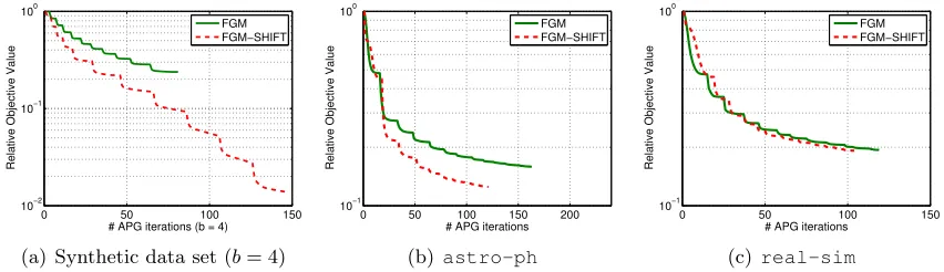
Warm Start: From Theorem 4, the number of iterations needed by APG to achieve an -solution isO(||ω0√−ω∗||
). Since FGM incrementally includes a set of features into the
subproblem optimization, an warm start ofω0 can be very useful to improve its efficiency. To be more specific, when a new active constraint is added, we can use the optimal solution of the last iteration (denoted by [ω∗10, ...,ω∗t−10]) as an initial guess to the next iteration. In other words, at the tth iteration, we use ω−1 =ω0 = [ω∗10, ...,ω∗t−1
0
5.3 De-biasing of FGM
Based on Algorithm 4, we show that FGM resembles the re-training process and can achieve de-biased solutions. For convenience, we first revisit the de-biasing process in the
`1-minimization (Figueiredo et al., 2007).
De-biasing for `1-methods. To reduce the solution bias, a de-biasing process is often adopted in `1-methods. For example, in the sparse recovery problem (Figueiredo et al.,
2007), after solving the`1-regularized problem, aleast-square problem(which drops the `1-regularizer) is solved with the detected features (or supports). To reduce the feature selection bias, one can also apply this de-biasing technique to the`1-SVM for classification
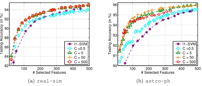
tasks. However, it is worth mentioning that, when dealing with classification tasks, due to the label noises, such as the rounding errors of labels, a regularizer is necessary and important to avoid the over-fitting issue. Alternatively, we can apply the standard SVM on the selected features to do the de-biasing using a relative large C, which is also referred to as the re-training. When C goes to infinity, it is equivalent to minimize the empirical loss without any regularizer, which, however, may cause the over-fitting problem.
De-biasing effect of FGM. Recall that, in FGM, the parameters B and the trade-off parameter C are adjusted separately. In the worst-case analysis, FGM includes B
features/groups that violate the optimality condition the most. When B is sufficiently small, the selected B features/groups can be regarded as the most relevant features. After that, FGM addresses the `22,1-regularized problem (22) w.r.t. the selected features only, which mimics the above re-training strategy for de-biasing. Specifically, we can use a relatively large C to penalize the empirical loss to reduce the solution bias. Accordingly, with a suitableC, each outer iteration of FGM can be deemed as the de-biasing process, and the de-biased solution will in turn help the worst-case analysis to select more discriminative features.
5.4 Stopping Conditions
Suitable stopping conditions of FGM are important to reduce the risk of over-fitting and improve the training efficiency. The stopping criteria of FGM include 1) the stopping conditions for the outer cutting plane iterations in Algorithm 1; 2) the stopping conditions for the inner APG iterations in Algorithm 4.
5.4.1 Stopping Conditions for Outer iterations
We first introduce the stopping conditions w.r.t. the outer iterations in Algorithm 1. Re-call that the optimality condition for the SIP problem is P
dt∈Dµt∇αf(α,dt) = 0 and
µt(f(α,dt)−fm(α)) = 0,∀dt∈ D. A direct stopping condition can be written as:
f(α,d)≤fm(α) +, ∀d∈ D, (26)
wherefm(α) = maxdh∈Ctf(α,dh) andis a small tolerance value. To check this condition, we just need to find a new dt+1 via the worst-case analysis. If f(α,dt+1) ≤ fm(α) +
, the stopping condition in (26) is achieved. In practice, due to the scale variation of
decreases. Therefore, in this paper, we propose to use the relative function value difference as the stopping condition instead:
F(ωt−1, b)−F(ωt, b)
F(ω0, b) ≤c, (27)
wherec is a small tolerance value. In some applications, one may need to select a desired
number of features. In such cases, we can terminate Algorithm 1 after a maximum number of T iterations with at mostT B features being selected.
5.4.2 Stopping Conditions for Inner iterations
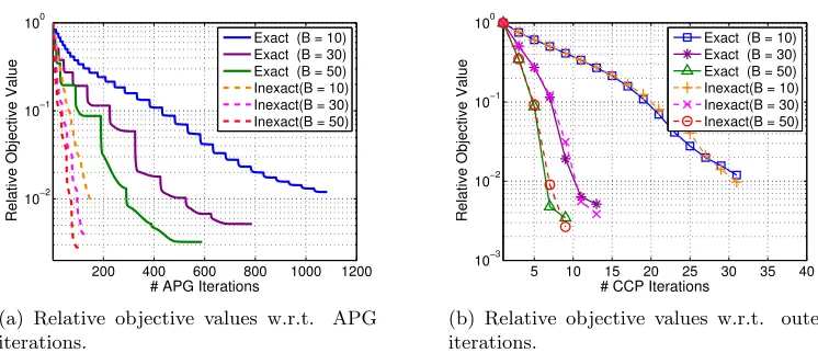
Exact and Inexact FGM: In each iteration of Algorithm 1, one needs to do the inner master problem minimization in (22). The optimality condition of (22) is ∇ωF(ω) = 0. In practice, to achieve a solution with high precision to meet this condition is expensive. Therefore, we usually achieve an-accurate solution instead.
Nevertheless, an inaccurate solution may affect the convergence. To demonstrate this, let ωb and bξ be the exact solution to (22). According to Theorem 3, the exact solution of
b
α to (20) can be obtained byαb =bξ. Now supposeω is an-accurate solution to (22) and
ξ be the corresponding loss, then we have αi=αbi+i, wherei is the gap between αb and
α. When performing the worst-case analysis in Algorithm 2, we need to calculate
c=
n
X
i=1
αiyixi= n
X
i=1
(αbi+i)yixi =bc+
n
X
i=1
iyixi=bc+ ∆bc,
wherebcdenotes the exact feature score w.r.t. αb, and ∆bcdenotes the error ofc brought by the inexact solution. Apparently, we have
|bcj−cj|=|∆cbj|=O(), ∀j= 1, ..., m.
Since we only need to find those significant features with the largest|cj|0s, a sufficiently small
is enough such that we can find the most-active constraint. Therefore, the convergence of FGM will not be affected ifis sufficiently small, but overall convergence speed of FGM can be greatly improved. Let {ωk} be the inner iteration sequence, in this paper, we set the stopping condition of the inner problem as
F(ωk−1)−F(ωk)
F(ωk−1) ≤in, (28)
where in is a small tolerance value. In practice, we set in = 0.001, which works well for
the problems that will be studied in this paper.
5.5 Cache for Efficient Implementations
The optimization scheme of FGM allows to use some cache techniques to improve the optimization efficiency.
one needs to calculatew0xi for each instance to compute the gradient of the loss function,
which takesO(mn) cost in general. Unlike these methods, the gradient computation in the modified APG algorithm of FGM is w.r.t. the selected features only. Therefore, we can use a column-based database to store the data, and cache these features in the main memory to accelerate the feature retrieval. To cache these features, we needs O(tBn) additional memory. However, the operation complexity for feature retrieval can be significantly re-duced from O(nm) to O(tBn), wheretB m for high dimensional problems. It is worth mentioning that, the cache for features is particularly important for the nonlinear feature selection with explicit feature mappings, where the data with expanded features can be too large to be loaded into the main memory.
Cache for inner products. The cache technique can be also used to accelerate the Algorithm 4. To make a sufficient decrease of the objective value, in Algorithm 4, a line search is performed to find a suitable step size. When doing the line search, one may need to calculate the loss function P(ω) many times, where ω = Sτ(g) = [ω01, ...,ω0t]0. The
computational cost will be very high if n is very large. However, according to equation (25), we have
ω=Sτ(gh) =
oh
||gh||
gh =
oh
||gh||
(vh−
1
τ∇P(vh)),
where onlyoh is affected by the step size. Then the calculation of
Pn
i=1ω 0x
i follows
n
X
i=1
ω0xi = n X i=1 t X h=1
ω0hxih
! = n X i=1 t X h=1 oh
||gh||
v0hxih −
1
τ ∇P(vh) 0x
ih
! .
According to the above calculation rule, we can make a fast computation of Pn
i=1ω0xi
by caching v0hxih and ∇P(vh)0xih for the hth group of each instance xi. Accordingly, the
complexity of computingPn
i=1ω 0x
i can be reduced fromO(ntB) to O(nt). That is to say,
no matter how many line search steps will be conducted, we only need to scan the selected features once, which can greatly reduce the computational cost.
6. Nonlinear Feature Selection Through Kernels
By applying the kernel tricks, we can extend FGM to do nonlinear feature selections. Let
φ(x) be a nonlinear feature mapping that maps the input features with nonlinear relations into a high-dimensional linear feature space. To select the features, we can also introduce a scaling vectord∈ Dand obtain a new feature mappingφ(x√d). By replacing (x√d) in (5) with φ(x√d), the kernel version of FGM can be formulated as the following semi-infinite kernel (SIK) learning problem:
min
α∈A,θθ : θ≥fK(α,d), ∀ d∈ D,
wherefK(α,d) =12(αy)0(Kd+C1I)(αy) andKijd is calculated asφ(xi
√
d)0φ(xj
√ d). This problem can be solved by Algorithm 1. However, we need to solve the following optimization problem in the worst-case analysis:
max d∈D 1 2 n X i=1
αiyiφ(xi
√ d) 2 = max d∈D 1
2(αy)
0
6.1 Worst Case Analysis for Additive Kernels
In general, solving problem (29) for general kernels (e.g., Gaussian kernels) is very challeng-ing. However, foradditive kernels, this problem can be exactly solved. A kernelKd is an additive kernel if it can be linearly represented by a set of base kernels{Kj}pj=1 (Maji and Berg, 2009). If each base kernel Kj is constructed by one feature or a subset of features,
we can select the optimal subset features by choosing a small subset of kernels.
Proposition 2 The worst-case analysis w.r.t. additive kernels can be exactly solved.
Proof Suppose that each base kernelKj in an additive kernel is constructed by one feature
or a subset of features. Let G = {G1, ...,Gp} be the index set of features that produce the
base kernel set {Kj}pj=1 and φj(xiGj) be the corresponding feature map to Gj. Similar to the group feature selection, we introduce a feature scaling vector d ∈ D ⊂ Rp to scale φj(xiGj). The resultant model becomes:
min d∈Db
min w,ξ,b
1 2kwk
2 2+
C
2
n
X
i=1 ξi2
s.t. yi
p
X
j=1 p
djw0Gjφj(xiGj)−b
≥1−ξi, ξi≥0, i= 1,· · · , n,
wherewGj has the same dimensionality withφj(xiGj). By transforming this problem to the SIP problem in (13), we can solve the kernel learning (selection) problem via FGM. The corresponding worst-case analysis is reduced to solve the following problem:
max d∈D
p
X
j=1
dj(αy)0Kj(αy) = max
d∈D
p
X
j=1 djsj,
wheresj = (αy)0Kj(αy) andKi,kj =φj(xiGj)
0φ
j(xkGj). This problem can be exactly solved by choosing the B kernels with the largestsj’s.
In the past decades, many additive kernels have been proposed based on specific application contexts, such as the general intersection kernel in computer vision (Maji and Berg, 2009), string kernel in text mining and ANOVA kernels (Bach, 2009). Taking the general inter-section kernel for example, it is defined as: k(x,z, a) =Pp
j=1min{|xj|a,|zj|a},wherea >0
is a kernel parameter. When a= 1, it reduces to the well-known Histogram Intersection Kernel (HIK), which has been widely used in computer vision and text classifications (Maji and Berg, 2009; Wu, 2012).
6.2 Worst-Case Analysis for Ultrahigh Dimensional Big Data
Ultrahigh dimensional big data widely exist in many application contexts. Particularly, in the nonlinear classification tasks with explicit nonlinear feature mappings, the dimension-ality of the feature space can be ultrahigh. If the explicit feature mapping is available, the nontrivial nonlinear feature selection task can be cast as a linear feature selection problem in the high-dimensional feature space.
Taking the polynomial kernelk(xi,xj) = (γx0ixj+r)υ for example, the dimension of the
feature mapping exponentially increases withυ(Chang et al., 2010), whereυ is referred to as the degree. Whenυ= 2, the 2-degree explicit feature mapping can be expressed as
φ(x) = [r,p2γrx1, ...,p2γrxm, γx21, ..., γx2m,
√
2γx1x2, ..., √
2γxm−1xm].
The second-order feature mapping can capture the feature pair dependencies, thus it has been widely applied in many applications such as text mining and natural language pro-cessing (Chang et al., 2010). Unfortunately, the dimensionality of the feature space is (m+ 2)(m+ 1)/2 and can be ultrahigh for a medianm. For example, if m = 106, the di-mensionality of the feature space isO(1012), and around 1 TB memory is required to store the weight vector w. As a result, most of the existing methods are not applicable (Chang et al., 2010). Fortunately, this computational bottleneck can be effectively avoided by FGM since only tB features are required to be stored in the main memory. For convenience, we store the indices and scores of the selectedtB features in a structured arraycB.
Algorithm 5Incremental Implementation of Algorithm 2 for Ultrahigh Dimensional Data. Given α,B, number of data groups k, feature mappingφ(x) and a structured arraycB.
1: SplitX intok subgroupsX= [X1, ...,Xk]. 2: For j= 1, ..., k.
Calculate the feature scores w.r.t. Xj according toφ(xi).
Sort sand update cB.
Fori=j+ 1, ..., k. (Optional)
Calculate the cross feature score sw.r.t. Xj and Xi. Sort s and update cB.
End End
3: Return cB.
For ultrahigh dimensional big data, it can be too huge to be loaded into the main memory, thus the worst-case analysis is still very challenging to be addressed. Motivated by the incremental worst-case analysis for complex group feature selection in Section 4.3, we propose to address the big data challenge in an incremental manner. The general scheme for the incremental implementation is presented in Algorithm 5. Particularly, we partition
7. Connections to Related Studies
In this section, we discuss the connections of proposed methods with related studies, such as the`1-regularization (Jenatton et al., 2011a), active set methods (Roth and Fischer, 2008;
Bach, 2009), SimpleMKL (Rakotomamonjy et al., 2008), `q-MKL (Kloft et al., 2009, 2011;
Kloft and Blanchard, 2012), infinite kernel learning (IKL) (Gehler and Nowozin, 2008), SMO-MKL (Vishwanathan et al., 2010), and so on.
7.1 Relation to `1-regularization
Recall that the `1-norm of a vector w can be expressed as a variational form (Jenatton
et al., 2011a):
kwk1 =
m
X
j=1 |wj|=
1 2mind0
m
X
j=1 wj2
dj
+dj. (30)
It is not difficult to verify that, d∗j =|wj| holds at the optimum, which indicates that the
scale of d∗j is proportional to |wj|. Therefore, it is meaningless to impose an additional
`1-constraint ||d||1 ≤ B or ||w||1 ≤ B in (30) since both d and w are scale-sensitive. As
a result, it is not so easy for the `1-norm methods to control the number of features to be selected as FGM does. On the contrary, in AFS, we bound d∈[0,1]m.
To demonstrate the connections of AFS to the`1-norm regularization, we need to make some transformations. Let wbj =wj
p
dj and wb = [wb1, ...,wbm]
0, the variational form of the
problem (5) can be equivalently written as
min d∈D min
b
w,ξ,b 1 2
m
X
j=1 b w2j
dj
+C 2
n
X
i=1 ξi2
s.t. yi(wb 0x
i−b)≥1−ξi, i= 1,· · · , n.
For simplicity, hereby we drop the hat fromwb and define a new regularizerkwk 2
B as
kwk2B= min d0
m
X
j=1 w2j
dj
, s.t. ||d||1 ≤B, d∈[0,1]m. (31)
This new regularizer has the following properties.
Proposition 3 Given a vector w∈ Rm with kwk0 =κ >0, where κ denotes the number
of nonzero entries in w. Let d∗ be the minimizer of (31), we have: (I) d∗j = 0 if |wj|= 0. (II) If κ ≤ B, then d∗j = 1 for |wj| > 0; else if kwk1
max{|wj|} ≥ B and κ > B, then we have
|wj|
d∗
j =
kwk1
B for all |wj|>0. (III) If κ≤B, then kwkB =kwk2; else if
kwk1
max{|wj|} ≥B and κ > B, kwkB= k√wBk1.
The proof can be found in Appendix D.
According to Proposition 3, if B < κ, kwkB is equivalent to the `1-norm regularizer.
by 1, which lead to two advantages of kwk2
B over the`1-norm regularizer. Firstly, by using kwk2
B, the sparsity and the over-fitting problem can be controlled separately by FGM.
Specifically, one can choose a proper C to reduce the feature selection bias, and a proper stopping tolerance c in (27) or a proper parameter B to adjust the number of features
to be selected. Conversely, in the `1-norm regularized problems, the number of features is determined by the regularization parameter C, but the solution bias may happen if we intend to select a small number of features with a small C. Secondly, by transforming the resultant optimization problem into an SIP problem, a feature generating paradigm has been developed. By iteratively infer the most informative features, this scheme is particularly suitable for dealing with ultrahigh dimensional big data that are infeasible for the existing
`1-norm methods, as shown in Section 6.2.
Proposition 3 can be easily extended to the group feature selection cases and multiple kernel learning cases. For instance, given a w ∈ Rm with p groups {G
1, ...,Gp}, we have
Pp
j=1||wGj||2 = kvk1, where v = [||wG1||, ...,||wGp||]
0 ∈
Rp. Therefore, the above two advantages are also applicable to FGM for group feature selection and multiple kernel learning.
7.2 Connection to Existing AFS Schemes
The proposed AFS scheme is very different from the existing AFS schemes (e.g., Weston et al., 2000; Chapelle et al., 2002; Grandvalet and Canu, 2002; Rakotomamonjy, 2003; Varma and Babu, 2009; Vishwanathan et al., 2010). In existing works, the scaling vectord0 d
is not upper bounded. For instance, in the SMO-MKL method (Vishwanathan et al., 2010), the AFS problem is reformulated as the following problem:
min
d0αmax∈A 1 0α−1
2
p
X
j=1
dj(αy)0Kj(αy) +
λ
2(
X
j
dqj)2q,
where A ={α|0 α C1,y0α = 0} and Kj denote a sub-kernel. When 0 ≤ q ≤ 1, it
induces sparse solutions, but results in non-convex optimization problems. Moreover, the sparsity of the solution is still determined by the regularization parameterλ. Consequently, the solution bias inevitably exists in the SMO-MKL formulation.
A more related work is the `1-MKL (Bach et al., 2004; Sonnenburg et al., 2006) or the
SimpleMKL problem (Rakotomamonjy et al., 2008), which tries to learn a linear combina-tion of kernels. The variacombina-tional regularizer of SimpleMKL can be written as:
min d0
p
X
j=1 ||wj||2
dj
, s.t. ||d||1≤1,
where p denotes the number of kernels and wj represents the parameter vector of the
jth kernel in the context of MKL (Kloft et al., 2009, 2011; Kloft and Blanchard, 2012). Correspondingly, the regularizer||w||2
B regarding kernels can be expressed as:
min d0
p
X
j=1 ||wj||2
dj
To illustrate the difference between (32) and the`1-MKL, we divide the two constraints in
(32) byB, and obtain
p
X
j=1 dj
B ≤1, 0≤ dj
B ≤
1
B,∀j∈ {1, ..., p}.
Clearly, the box constraint dj
B ≤
1
Bmakes (32) different from the variational regularizer in`1
-MKL. Actually, the`1-norm MKL is only a special case of||w||2
BwhenB = 1. Moreover, by
extending Proposition 3, we can obtain that ifB > κ, we have||w||2
B =
Pp
j=1||wj||2, which
becomes a non-sparse regularizer. Another similar work is the `q-MKL, which generalizes
the `1-MKL to `q-norm (q > 1) (Kloft et al., 2009, 2011; Kloft and Blanchard, 2012).
Specifically, the variational regularizer of `q-MKL can be written as
min d0
p
X
j=1 ||wj||2
dj
, s.t. ||d||2q≤1.
We can see that, the box constraint 0≤ dj
B ≤
1
B,∀j ∈ {1, ..., p} is missing in the `q-MKL.
However, when q >1, the`q-MKL cannot induce sparse solutions, and thus cannot discard
non-important kernels or features. Therefore, the underlying assumption for`q-MKL is that,
most of the kernels are relevant for the classification tasks. Finally, it is worth mentioning that, when doing multiple kernel learning, both `1-MKL and `q-MKL require to compute
and involve all the base kernels. Consequently the computational cost is unbearable for large-scale problems with many kernels.
An infinite kernel learning method is introduced to deal with infinite number of ker-nels (p = ∞) (Gehler and Nowozin, 2008). Specifically, IKL adopts the `1-MKL
formu-lation (Bach et al., 2004; Sonnenburg et al., 2006), thus it can be considered as a special case of FGM when setting B = 1. Due to the infinite number of possible constraints, IKL also adopts the cutting plane algorithm to address the resultant problem. However, it can only include one kernel per iteration; while FGM can include B kernels per iteration. In this sense, IKL is also analogous to the active set methods (Roth and Fischer, 2008; Bach, 2009). For both methods, the worst-case analysis for large-scale problems usually domi-nates the overall training complexity. For FGM, since it is able to include B kernels per iteration, it obviously reduces the number of worst-case analysis steps, and thus has great computational advantages over IKL. Finally, it is worth mentioning that, based on the IKL formulation, it is non-trivial for IKL to include B kernels per iteration.
7.3 Connection to Multiple Kernel Learning