A Note on Polynomial type Minimal Surfaces

(1)

Annals. Computer Science Series. 12 Tome 1 Fasc. – 2014

A

N

O

T

E

O

N

P

O

L

Y

N

O

M

I

A

L

T

Y

P

E

M

I

N

I

M

A

L

S

U

R

F

A

C

E

S

C

Ch

hi

i

ra

r

ag

g

D

De

ee

e

pa

p

ak

k

A

Ag

g

r

aw

a

w

al

a

l

,

P

Pr

r

as

a

s

an

a

nn

na

a

K

Ku

um

m

ar

a

r

Birla Institute of Technology and Science Pilani K K Birla Goa Campus , Department of Mathematics

ABSTRACT:In this paper, we develop two new minimal surfaces of degree six in parametric polynomial form with isothermal parameter. Graphical representations in different angles have been presented. All computations are done using Mathematica 9.0.

KEYWORDS: Minimal Surface, Polynomials, Euclidean Space.

1.

INTRODUCTION

The study of minimal surfaces is indispensable to Differential Geometry. In fact minimal surfaces or the surfaces of least area, are a field of study that has intrigued mathematicians for many years. The inspiration stems from the fact that they can easily be visualized. The famous physicist J. A. F. Plateau, studied them experimentally and determined some interesting geometric properties. A major breakthrough in the study of minimal surfaces has been established in evolving important theory with the works of J. Douglas [Dou30] and T. Radó [Rad30].

Finding minimal surfaces is a herculean task and in general still an open problem. Thus only a few exact minimal surfaces have been found, and computational techniques could be used as an inevitable tool for the advancement of the branch. The only global result which was an exception to the above argument is the work by Bernstein [Ber27], who considered minima l surfaces from the point of view of PDE.

Much of the work in the twentieth century has involved generalizations of the theory to higher dimensions, Riemannian spaces and wider classes of surfaces. One of the most important works is that of Osserman [Oss64, Oss69] which has greatly influenced the modern global theory of complete minimal surfaces in three dimensional Euclidean spaces. Costa [Cos84] discovered a new complete embedded minimal surface of genus 1 with three punctures. This famous work disproved the conjecture that the plane, the helicoid and the catenoid are the only embedded minimal surfaces that could be formed by puncturing a compact surface. More recent work includes the discovery of a sequence of properly embedded minimal surfaces with finite topology by Hoffman [Hof87, HM90] and Meeks [HM90], and significant contributions by Karcher [Kar88], and Pérez and Ros [PR96]. Brakke [Bra92], Hinata et al. [HSK74] and Wagner [Wag77], evolved some parametric minimal surfaces, using

finite element methods.

The theory of minimal surfaces has found applications in many fields such as architecture [Emm13, Wal09], material science, aviation, ship manufacture, general relativity [CGP10], biology, crystallogeny, art [Emm93] and so on. Triply periodic minimal surfaces have been observed in biological membranes [DM98], equipotential surfaces in crystals [Mac85], and as block copolymers [JGA03] and nanocomposites.

In this paper, we explore an elegant technique given by Xu and Wang [XW08] to generate new minima l surfaces of degree six in parametric polynomial form with isothermal parameters, and provide our construction of two new sets of minimal surfaces. 2. PRELIMINARY

Before we generate the new minimal surfaces, we will first review some important definitions, concepts and results that we will require [ Giu84, Pre01]. Let σ be a regular surface patch in R3 given by:

σ(u, v) = (x(u, v), y(u, v), z(u, v)), where u, v are in R.

We need the following fundamental definitions from differential geometry which play a crucial role in determining the nature of surfaces.

Definition 1. The first fundamental form of σ is defined as:

Edu2 + 2Fdudv + Gdv2

where

E = σu∙ σu,F = σu∙ σv,G = σv ∙ σv

Here,σuand σv are the first-order partial derivatives of σ(u, v) with respect to u and v respectively.

Definition 2. The second fundamental form of σ is defined as:

Ldu2 + 2Mdudv + Ndv2

(2)

Here N is the standard unit normal vector on the surface and σuu, σuv and σvv are the second order partial derivatives of σ(u, v) with respect to u and v. Definition 3. The mean curvature H of σ(u, v) is define d as:

Definition 4. If the surface σ(u, v) satisfies: E = G, F = 0,

then σ(u, v) is called a surface with isothermal parameter.

Definition 5. If the surface σ(u, v) satisfies: σuu + σvv = 0,

then σ(u, v) is called a harmonic surface. Definition 6. If σ(u, v) satisfies :

H = 0,

then σ(u, v) is called a minimal surface.

Before proceeding further we state few lemmas [XW08] which are required in the subsequent section. Lemma 1. A surface with isothermal parameter is a minimal surface if and only if it is a harmonic surface.

Lemma 2. A harmonic polynomial surface of degree six,σ(u, v) must have the following form:

where a, b, c, d, e, f, g, h, i, j, k, l, m are coefficient vectors.

We start by giving a close relation between minima l surfaces and harmonic polynomials. In [ XW08], a very significant theorem has been proved on the necessary and sufficient conditions, for a harmonic polynomial surface of degree six to be minimal. Theorem 1. A harmonic polynomial surface of degree six, σ(u, v) is a minimal surface if and only if

equations:

3. GENERATING NEW MINIMAL SURFACES

To generate a new minimal surface from harmonic polynomial surfaces, we must find a solution to the system of e quations given in Theorem 1. However, it is extremely difficult to get the solution for the system directly. We therefore start by arbitrarily initializing values to some of the coefficient vectors and then make intelligent assumptions to satisfy the other equations. The paper [ XW08] gives examples of two such classes of minimal surfaces and studies their properties. In this paper we generate two different classes of minimal surfaces.

3.1 Harmonic polyno mial minimal surface 1

We make the following assumptions:

(3)

.

Next, to find i and j we make an intelligent assumption to satisfy their corresponding equations :

i= (1, 1, 0) j = (-2, 2, 0) Similarly, we find a, b, c and d;

a = (1, 0, 0), b = (0, 2, 0),

c = (1, 1, 0), d = (-1, 1, 0)

We directly get four reduced equations for e, f, g and

h as the following:

Substituting and solving the remaining equations yields the following values for the coefficient vectors

f, g and h in terms of the components of vector e = (e1, e2, e3):

We now substitute these values for the coefficient vectors in the equation given in Lemma 2 for σ(u, v). We can safely assume m = (0, 0, 0) since it is a constant vector and does not affect the shape of the surface. The components of e act as the control parameters for the shape of the surface.

We choose e1 = 0, e2 = 0 and e3 = -30.

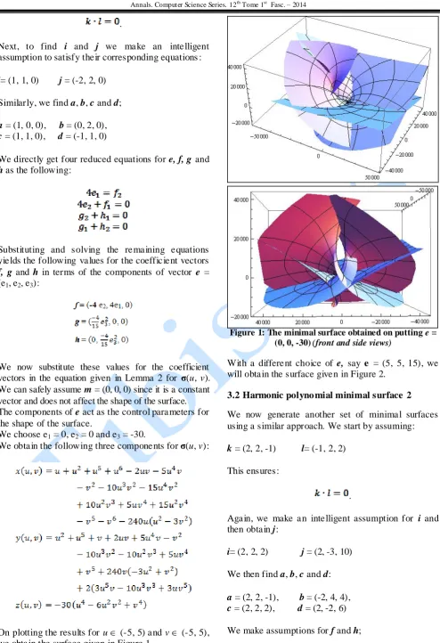
We obtain the following three components forσ(u, v):

On plotting the results for u (-5, 5) and v (-5, 5), we obtain the surface given in Figure 1.

Figure 1: The minimal surface obtained on putting e = (0, 0, -30) (front and side views)

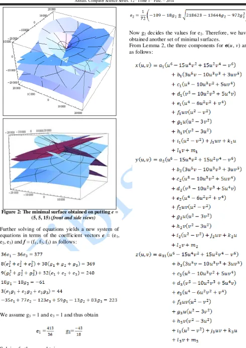
With a different choice of e, say e = (5, 5, 15), we will obtain the surface given in Figure 2.

3.2 Harmonic polyno mial minimal surface 2

We now generate another set of minimal surfaces using a similar approach. We start by assuming:

k = (2, 2, -1) l= (-1, 2, 2) This ensures:

.

Again, we make an intelligent assumption for i and then obtain j:

i= (2, 2, 2) j = (2, -3, 10) We then find a, b, c and d:

a = (2, 2, -1), b = (-2, 4, 4),

c = (2, 2, 2), d = (2, -2, 6) We make assumptions for f and h;

(4)

Figure 2: The minimal surface obtained on putting e = (5, 5, 15) (front and side views)

Further solving of equations yields a new system of equations in terms of the coefficient vectors e = (e1,

e2, e3) and f = (f1, f2, f3) as follows:

We assume g3 = 1 and e3 = 1 and thus obtain

Solving further, we obtain:

Now g2 decides the values for e2. Therefore, we have

obtained another set of minimal surfaces.

From Lemma 2, the three components for σ(u, v) are as follows:

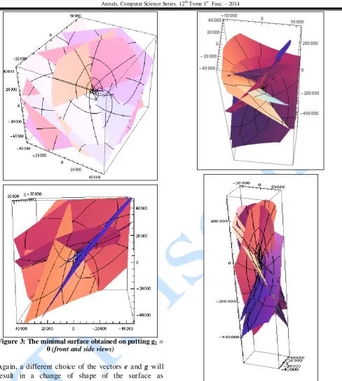
Taking m = (0, 0, 0) and putting g2 = 0, we obtain the

(5)

Figure 3: The minimal surface obtained on putting g2 = 0 (front and side views)

Again, a different choice of the vectors e and g will result in a change of shape of the surface as

illustrated in Figure 4. _{Figure 4. The minimal surface obtained with e1 = 413} and g2 = 0(front and side views)

4. CONCLUSION AND FUTURE WORK

(6)

REFERENCES

[Ber27] S. Bernstein - Übereingeometrisches Theorem und seine Anwendung auf die partiellenDifferentialgleichungenvomelli ptischenTypus, Math. Zet., 26, 551-558, 1927.

[Bra92] K. A. Brakke - The surface evolver,

Exp. Math.,1 (2), 141–165, 1992. [CGP10] P. T. Chruściel, G. J. Gallo way, D.

Pollack - Mathematical general relativity: a sampler, Bull. Amer. Math. Soc.,47, 567-638, 2010.

[Cos84] C. J. Costa - Example of a complete minimal immersion in R3 of genus one and three embedded ends, Bol. Soc. Bras. Math. , 15, 47–54, 1984.

[DM98] Y. Deng, M. Mieczkowski - Three-dimensional periodic cubic membrane structure in the mitochondria of amoebae Chaoscarolinensis, Protoplasma, 203, 16–25, 1998.

[Dou30] J. Douglas - Solution of the problem of Plateau, Proc. Nat.Aca. Sci., 16, 242– 248, 1930.

[Emm13] M. Emmer - Minimal Surfaces and Architecture: New Forms, Nex. Net. Jl., 15, 227-239, 2013.

[Emm93] M. Emmer - Soap Bubbles in Art and Science: From the Past to the Future of Math Art, The Visual Mind, 135 – 142, 1993.

[Giu84] E. Giusti - Minimal Surfaces and functions of bounded variation, Birkhauser-Verlag, Basel-Boston, 1984. [HM90] D. Hoffman, W. H. Meeks III -

Embedded minimal surfaces of finite topology, Ann. Math.,131, 1–34, 1990. [Hof87] D. Hoffman - The co mputer-aided

discovery of new embedded minimal surfaces, Math.Intell.,9, 8-21, 1987. [HSK74] M. Hinata, M. Shimasaki, T. Kiyono -

Numerical solution of Plateau’s problem by a finite element method, Math. Comp., 28 (125), 45–60, 1974.

[JGA03] S. Jiang, A. Göpfert, V. Abetz - Novel Morphologies of Block Copolymer

Blends via Hydrogen Bonding,

Macromolecules , 36, 6171–6177, 2003. [Kar88] H. Karcher - Embedded minimal

surfaces derived from Scherk's

examples, Man. Math., 62, 83-114, 1988.

[Mac85] A. L. Mackay - Periodic minimal surfaces, Nature, Lond., 314, 604-606, 1985.

[Oss64] R. Ossermann - Global properties of minimal surfaces in E3 and En, Ann. Math., 80, 340–364, 1964.

[Oss69] R. Ossermann - A Survey of Minimal Surfaces, Van Nostrand, Reinhold, New York, 1969.

[PR96] J. Pérez, A. Ros - The space of properly embedded minimal surfaces with finite total curvature, Indiana Univ. Math. J., 45, 177-204, 1996.

[Pre01] A. N. Pressley- Elementary Differential Geometry, Springer-Verlag, London, 2001.

[Rad30] T. Radó - On Plateau’s problem, Ann. Math.,31 (3), 457–469, 1930.

[Wag77] H. J. Wagner - A contribution to the numerical approximation of minimal surfaces, Computing, 19 (1), 35–58, 1977.

[Wal09] T. Wallisser - Other geometries in architecture: bubbles, knots and minimal surfaces, Mathknow, 3, 91-111, 2009. [XW08] G. Xu, G. Wang - Parametric