Applying queuing theory for a reliable integrated location –inventory problem under facility disruption risks

Journal of Industrial Engineering and Management Studies

Vol. 4, No. 2, 2017, pp. 1-18

DOI: 10.22116/JIEMS.2017.54601 www.jiems.icms.ac.ir

Applying queuing theory for a reliable integrated location

inventory problem under facility disruption risks

Masoud Rabbani1,*, Leila Aliabadi1_{, Razieh Heidari}1_{, Hamed Farrokhi-Asl}2

Abstract

This study considers a reliable location – inventory problem for a supply chain system comprising one supplier, multiple distribution centers (DCs), and multiple retailers in which we determine DCs location, inventory replenishment decisions and assignment retailers to DCs, simultaneously. Each DC is managed through a continuous review (S, Q) inventory policy. For tackling real world conditions, we consider the risk of probabilistic distribution center disruptions, and also uncertain demand and lead times, which follow Poisson and Exponential distributions, respectively. A new mathematical formulation is proposed and we model the proposed problem in two steps, in the first step, a queuing system is applied to calculate mean inventory and mean reorder rate of steady-state condition for each DC. Next, regarding the results obtained from the first step, we formulate a mixed integer nonlinear programming model which minimizes the total expected cost of inventory, location and transportation and can be solved efficiently by means of LINGO software. Finally, several test problems and sensitivity analysis of key parameters are conducted in order to illustrate the effectiveness of the proposed model.

Keywords: inventory – location model; disruption; queuing theory; uncertain demand; supply chain management.

Received: September 2016-23 Revised: June 2017-16 Accepted: July 2017-15

1.

Introduction

Supply chain management (SCM) is defined as a set of tactical, operational and strategic decision-making functions that optimizes the performance of whole supply chain (Zeng, Phan, & Matsui, 2013). Traditionally, researchers have considered the tactical decisions such as the inventory control and the strategic decisions such as facility locations separately that may lead to sub-optimal decisions (Daskin, Coullard, & Shen, 2002; Diabat, Abdallah, & Henschel, 2015; Javid & Azad, 2010; Miranda & Garrido, 2004). By considering these decisions at the same time, a significant saving in total cost can be achieved. Therefore, many

* Corresponding author; [email protected]

researchers have been interested in joint inventory and location models in order to obtain single optimization model for determining both tactical and strategic decisions, simultaneously. Baumol and Wolfe (1958) were the first researchers that suggested the idea of joint inventory systems and facility locations models. Shen, Coullard, and Daskin (2003) presented a joint inventory–location problem and considered an amount of safety stock in their models. Their problem was formulated as a set-covering integer programming model. An integrated location-distribution–inventory model for three-echelon supply chain under demand uncertainty is presented by Miranda and Garrido (2008).They solved the proposed problem by an efficient heuristic based on Lagrangian relaxation. Liao, Hsieh, and Lai (2011) investigated the effect of distribution, facility location, and inventory issues at the same time in a multi-objective location-inventory problem under vendor– management inventory. They applied a Non-Dominated Sorting Genetic Algorithm for solving their model. Lin, Yang, and Chang (2013) formulated a hub location-inventory model for a strategic design of bicycle sharing system. The main objective of their paper was to determine the following joint decisions: the number and locations of bicycle stations in the system, the creation of bicycle lanes among bicycle stations, the selection of paths of users between origins and destinations, and the inventory levels of sharing bicycles to be held at the bicycle stations. The design decisions are made with consideration for both total cost and service levels and optimized by a heuristic method. Gzara, Nematollahi, and Dasci (2014) developed two mixed-integer nonlinear problems for joint inventory and location decisions under part service level requirements and part warehouse. Such models are complex due to uncertain demand and extremely nonlinear time-based service level restrictions. Since they developed a new method for approximating these nonlinearities to a linear formulation which can be solved through commercial optimization software. Fontalvo, Maza, and Miranda (2017) presented a strategic inventory-location model, multi- item and different with demand periods and developed a genetic algorithm for solving model. Then, a case study of a steel company in Colombia was discussed to illustrate the proposed model.

In a supply chain planning decision process, uncertainty is the main factor which can affect the effectiveness of supply chain and also its performance (Macchion, Danese, & Vinelli, 2015). The source of uncertainty is categorized into three groups: manufacturing (process), supply, and demand. Recently, the effect of uncertainty in studying joint location- inventory problem has drawn more academic attention. For instance, Sadjadi, Makui, Dehghani, and Pourmohammad (2016) formulated a stochastic location- inventory problem with uncertain lead time and demand which follow Exponential and Poisson distributions, respectively. In their problem, shortages are allowed and are fully backlogged. They presented a nonlinear integer-programming model to address their stochastic problem and solved it by using CPLEX. A novel and practical stochastic inventory- location problem with stochastic demand under two different replenishment policies, independent replenishment and join replenishment, was proposed by Qu, Wang, and Liu (2015). They designed intelligent algorithms to solve their models and found that inventory- location problem with joint replenishment outperforms than inventory- location problem with independent replenishment while opening distribution center is more than one. Another stochastic location- inventory with uncertain demand was addressed by Zhang and Unnikrishnan (2016) for a closed loop supply chain. They formulated six different coordination strategies as nonlinear integer problems with chance restrictions and transformed to conic quadratic mixed-integer programs that can be efficiently solved by CPLEX.

comparison with traditional inventory models. The first research of queuing systems with inventory was done by Sigman and Simchi-Levi (1992). They proposed a light traffic heuristic for an M/G/1 - queue with a finite inventory when lead time follows Exponential distribution. Liu, Liu, and Yao (2004) suggested a multi-stage inventory queue model, which this queuing model incorporates an inventory control mechanism like the base stock level. Schwarz and Daduna (2006) analyzed an M/M/1 queuing system with inventory control, allowable shortages, and uncertain lead time under different continuous review such as (r, S), (r, Q) , and (0, Q). Kim (2005) considered an inventory control problem with lost sales in a facility that presents a single kind of service for customers. He modeled the proposed problem using a queuing system with limited waiting room and on- instantaneous replenishment policy. A queuing – inventory system with two groups of customers was addressed by Zhao and Lian (2011). They computed the steady-state probability distribution by using Bright–Taylor algorithm through formulating their model as a level –dependent quasi-birth-and-death method. Saffari and Haji (2009) studied a queuing system with inventory control for two – echelon supply chain where demand rate is Poisson distribution and the supplier applies a continuous review (r, Q) policy. They suggested that if the supplier confronts shortage, the retailer can buy the product from others suppliers with zero lead times and an extra cost. An (S,Q) Markovian inventory system with two kinds of customers, ordinary and priority customers, and lost sales was analyzed by Isotupa (2006). He assumed the demand rate for each kind of customer is Poisson distribution with different and independent parameters. Then, their model was developed by Isotupa and Samanta (2013) using the concepts of rationing in which a supplier reserve several stocks for priority customers. In situations that on –hand inventory drops below a certain level, k, all existing inventory reserved for priority customers and all demand of ordinary customers will lose. Teimoury, Modarres, Ghasemzadeh, and Fathi (2010) applied a queuing approach to production-inventory planning considering two class of customers, continuous review (S. Q) and lost sales in a PASHOO Chemical Company. In their model, each type of customer arrives according to two independent Poisson distribution with parameters λ₁ and λ₂for priority customers and ordinary, respectively, and lead times are exponentially distributed with parameter μ. They initially developed an algorithm to determine the optimal values order quantity, Q, and reorder level, S. Then, a multi-item capacitated lot-sizing problem with safety stock and setup times production planning model is formulated for determining the production quantity at each period by using optimal reorder level and quantity calculated by first algorithm as inputs. RAMEZANI (2014), Krishnamoorthy, Shajin, and Lakshmy (2016), Melikov and Shahmaliyev (2017), and Ghafour, Ramli, and Zaibidi (2017) also developed a queuing – inventory system with different assumptions.

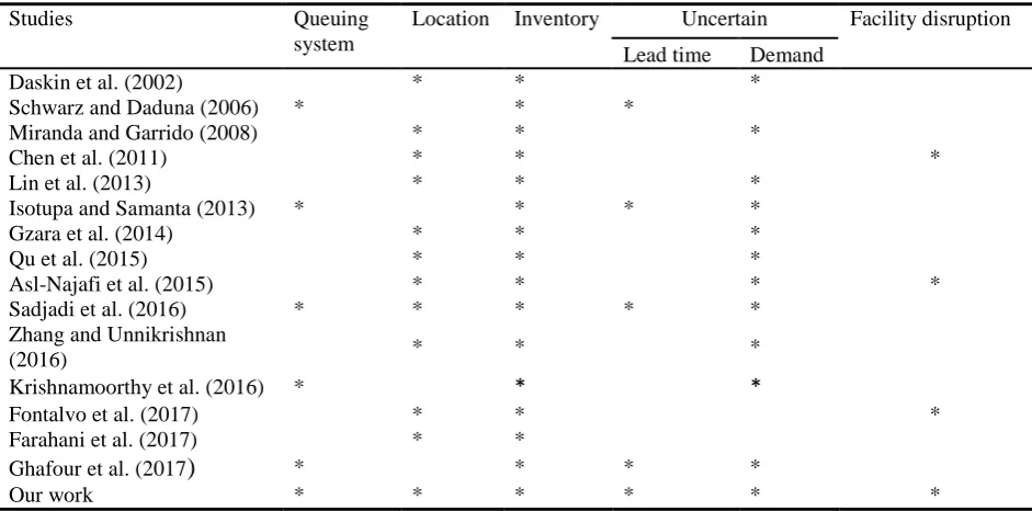
facilities may fail partially in case of disruption and considered substitutable products as a strategy to reduce the risk of disruption. Due to NP hard problem, they developed a hybrid algorithm including Variable Neighborhood Search and Tabu Search to solve their problem. A comparison of mentioned papers is illustrated in Table 1. From the Table, most previous papers on inventory -location models have failed to take into account the issue of facility disruption and uncertain lead time. Furthermore, papers that considered the risk of disruption, have failed to consider uncertain demand and lead time. However, uncertain demand, uncertain lead time and facility disruption may exist at the same time. Develop a model considering all of these issues are needed. Hence, we propose in this study a mixed integer nonlinear programing model (MINLP) to integrate a facility location and inventory system. This problem addresses a three levels supply chain with a supplier, multiple distributed centers (DCs) and multiple retailers. Demands from retailers arrive according to Poisson distribution with parameter λ. Supplier’s lead time is uncertain and follow exponential distribution with parameter μ. Each opened distribution center has an (S. Q)inventory policy. In order to make the proposed problem more realistic, we consider the risk of probabilistic DC disruptions in our model. This study uses a queuing system for calculating the mean inventory level and mean reorder rate of steady-state condition. Next, a reliable inventory– location model is formulated based on the results of queuing theory, which minimizes the total expected costs associated with inventory, location, and transportation. Our paper is the first one to consider the issues of uncertain demand, uncertain lead time, and the risk of facility disruption simultaneously in an integrated location- inventory problem.

The rest of our research is organized as follows: We first describe the problem in Section 2. Section 3 provides notations and model formulation. Then, we solve the proposed model using LINGO 9 software and present numerical examples and sensitivity analysis of important parameters respect to different numbers of retailers and distribution centers in Section 4. Finally, conclusion remarks and future works direction are provided in Section 5.

Table 1. Brief review of mentioned studies.

Studies Queuing

system

Location Inventory Uncertain Facility disruption Lead time Demand

Daskin et al. (2002) * * *

Schwarz and Daduna (2006) * * *

Miranda and Garrido (2008) * * *

Chen et al. (2011) * * *

Lin et al. (2013) * * *

Isotupa and Samanta (2013) * * * *

Gzara et al. (2014) * * *

Qu et al. (2015) * * *

Asl-Najafi et al. (2015) * * * *

Sadjadi et al. (2016) * * * * *

Zhang and Unnikrishnan

(2016) * * *

Krishnamoorthy et al. (2016) * * *

Fontalvo et al. (2017) * * *

Farahani et al. (2017) * *

Ghafour et al. (2017) * * * *

2.

Problem definition

This study presents a mathematical programming formulation for a reliable location- inventory problem in a three-level supply chain distribution system involving a single supplier, multiple distribution centers and multiple retailers. It is assumed that the location of retailers and supplier are predetermined. The formulation includes the following decisions: (і) locating distribution centers from a set of candidate locations 𝐽 (іі) the best assignment of retailers to opened distribution centers (ііі) the inventory policy at each opened distribution center. Each opened distribution center orders a single commodity to supplier based on an (𝑆. 𝑄) inventory policy that arrives after an exponentially distributed lead time with parameter 𝜇. Each retailer is only assigned to one opened distribution center. Retailers’ demands arrive according to a Poisson process and the retailers' demands are independent. Hence, the demand of each opened distribution center follows Poisson distributed with parameter 𝜆. Inventory management policy at each opened distribution center follows First In, Firs Out (FIFO) policy. Each candidate distribution center in set 𝐽 can disrupt independently with an equal probability 𝑝. When an opened distribution center fails, it cannot prepare any service and its original retailers will be either assigned to other opened distribution center (functional) or subject to certain penalty. Regarding Chen et al. (2011), it is assumed each retailer can get service from a serial of 𝑅 distribution centers. Under this assumption, in normal situations, each retailer will be assigned its Level 1 distribution center, called primary distribution center. Whenever, the retailer’s Level 𝑟 (𝑟 < 𝑅 − 1) distribution center is disrupted, the retailer is reassigned to its Level (𝑟 + 1) distribution center (backup distribution center) . When all of the assigned distribution center to the retailer are failed, the retailers give up service and incur a penalty cost. Thereupon, due to independent failures, the probability for a retailer to get service from its level-𝑟 facility is (1 − 𝑝)𝑝𝑟−1 and the probability for a retailer to suffer penalty is 𝑝𝑅. By considering this assumption, supply chain system reliability and overall performance would be significantly improved. So, the main objective is to minimize total cost of distribution center location, inventory management, and transportation. Figure 1 shows the supply chain described in this study.

DC 1

DC 4 DC 2

DC 3 supplier

Retailer 1

Retailer 2

3. Model formulation

In (S, Q) inventory policy, as soon as the stock on - hand drops the safety level, S, a batch of 𝑄(𝑄 > 𝑆) units is placed. So, the maximum level is 𝑄 + 𝑆. The constraint 𝑄 > 𝑆 guarantees that there exist no perpetual shortages. If 𝑄 ≤ 𝑆 and inventory level drops to zero then the system will be in shortage forever. As above mentioned, supplier’s lead time follows exponential distribution with parameter 𝜇 and, the demand of each opened distribution center is Poisson distributed with parameter𝜆. In this section a queuing system is applied to calculate mean inventory and the mean reorder rate in each opened distribution center.

We define 𝐼_𝑗(𝑡) as the inventory level in opened distribution center 𝑗 at time 𝑡. As regards 𝑄_𝑗 > 𝑆_𝑗, at any given point of time there exist at most one order pending. So, inventory level process {𝐼_𝑗(𝑡); 𝑡 ≥ 0} with state space as 𝐸_𝑗 = {0.1.2 … . 𝑄_𝑗 + 𝑆_𝑗} is a Markov process that the rate diagram of it is shown in Figure 2. So, the steady-state probabilities of the inventory system are calculated by following equations:

𝑃𝑗(𝑖. 𝑘. 𝑡) = 𝑝𝑟 [𝐼𝑗(𝑡) = 𝑘|𝐼𝑗(0) = 𝑖] 𝑖. 𝑘 𝜖 𝐸𝑗 (1)

𝑃𝑗(𝑘) = 𝑙𝑖𝑚_𝑡→∞𝑃𝑗(𝑖. 𝑘. 𝑡). (2)

0 1 k k+1 S S+1 K-1 k K+1 Q K-Q K-1 k K+1 S+Q

λ

λ λ λ λ λ λ λ λ λ λ λ λ λ

μ

μ

μ

... ... ... ... ... ... ...

Figure 2. Rate diagram for (S, Q) inventory policy

According to Figure 2 and Markov process properties, the balance equations for the system are given as follows:

𝜆_𝑗𝑃_𝑗(𝑆_𝑗+ 𝑄_𝑗) = 𝜇𝑃_𝑗(𝑆_𝑗)

𝜆_𝑗𝑃_𝑗(𝑘) = 𝜆𝑗𝑃𝑗(𝑘 + 1) + 𝜇𝑃𝑗(𝑘 − 𝑄𝑗) 𝑄𝑗 ≤ 𝑘 ≤ 𝑄𝑗+ 𝑆𝑗− 1

𝜆_𝑗𝑃_𝑗(𝑘) = 𝜆𝑗𝑃𝑗(𝑘 + 1) 𝑆𝑗+ 1 ≤ 𝑘 ≤ 𝑄𝑗 − 1

(𝜆_𝑗+ 𝜇)𝑃_𝑗(𝑆_𝑗) = 𝜆_𝑗𝑃_𝑗(𝑆_𝑗+ 1) ₍₃₎

(𝜆𝑗+ 𝜇)𝑃𝑗(𝑘) = 𝜆𝑗𝑃𝑗(𝑘 + 1) 1 ≤ 𝑘 ≤ 𝑆𝑗− 1

𝜇𝑃𝑗(0) = 𝜆𝑗𝑃𝑗(1)

By solving the above equations recursively, as a result:

𝑃𝑗(𝑘) = (1 +

𝜇 𝜆𝑗)

𝑘−1_𝜇

𝜆𝑗𝑃𝑗(0)

1 ≤ 𝑘 ≤ 𝑆𝑗 (4)

𝑃𝑗(𝑘) = (1 +

𝜇 𝜆_𝑗)

𝑆𝑗 _𝜇

𝜆_𝑗𝑃𝑗(0) 𝑆𝑗 ≤ 𝑘 ≤ 𝑄𝑗 (5)

𝑃_𝑗(𝑘) = ((1 + 𝜇 𝜆_𝑗)

𝑆𝑗

− (1 + 𝜇 𝜆_𝑗)

𝑘−𝑄𝑗−1 )𝜇

Since ∑𝑄_𝑘=0𝑗+𝑆𝑗𝑃_𝑗(𝑘) = 1 from equations (4) to (6), we have:

𝑃_𝑗(0) = 𝜆𝑗

𝜆_𝑗+ 𝜇𝑄_𝑗(1 +_𝜆𝜇 𝑗)

𝑆𝑗 ₍₇₎

Now, we can calculate the mean reorder, 𝑅_𝑗, rate and mean inventory level, 𝐼̅_𝑗, in the steady-state condition as below.

 The mean reorder rate in each distribution center (𝑅_𝑗)

𝑅_𝑗 = 𝜆_𝑗𝑃_𝑗(𝑆_𝑗 + 1) = 𝜇 (1 + 𝜇 𝜆_𝑗)

𝑆𝑗

𝑃_𝑗(0) (8)

 The mean inventory level in each distribution center (𝐼̅_𝑗)

𝐼̅𝑗 = ∑ 𝑘 × 𝑘∈𝐸𝑗

𝑃𝑗(𝑘) = (1 +

𝜇 𝜆𝑗)

𝑆_𝑗

((𝑄𝑗2 + 𝑄𝑗+ 2𝑄𝑗𝑆𝑗)

𝜇

2𝜆𝑗+ 𝑆𝑗+ 1) 𝑃𝑗(0)

− (1 + 𝜇 𝜆𝑗)

𝑆𝑗+1

(𝑄_𝑗+ 𝑆_𝑗+ 1)𝑃_𝑗(0) + (𝑄_𝑗+ 2)𝑃_𝑗(0) (9)

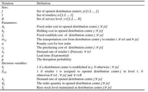
The sets, parameters and variables used in the proposed location-inventory problem are defined in Table 2. In next section, we first introduce component of the total cost function, then formulate the problem as a nonlinear mixed-integer model.

Table 2. Notations

Notation Definition

Sets:

𝐽 Set of opened distribution centers; 𝑗𝜖{1.2 … . 𝐽}

𝐼 Set of retailers; 𝑖𝜖{1.2 … . 𝐼}

𝑅 Set of service level ; 𝑟𝜖{1.2 … . 𝑅} Parameters:

𝐴_𝑗 Fixed order cost in opened distribution center 𝑗 ;∀ 𝑗𝜖𝐽

ℎ𝑗 Holding cost in opened distribution center 𝑗 ;∀ 𝑗𝜖𝐽

𝑓_𝑗 Fixed establish cost of distribution center 𝑗 ;∀ 𝑗𝜖𝐽

𝑡r𝑖𝑗 The transportation cost from distribution center 𝑗 to retailer 𝑖 ;∀ 𝑖𝜖𝐼 and ∀ 𝑗𝜖𝐽

𝜋 Penalty cost for lost order

𝑐_𝑗 The purchasing cost of distribution center 𝑗 ;∀ 𝑗𝜖𝐽

𝜆_𝑖 Demand rate of retailer 𝑖 (Poisson) ∀ 𝑖𝜖𝐼

𝜇 Lead time (Exponential)

𝑝 The disruption probability

Decision variables:

𝑌𝑗 1 if a distribution center is established in 𝑗, 0 otherwise ; ∀ 𝑗𝜖𝐽

𝑍_𝑖𝑗𝑟 1 if retailer 𝑖 is assigned to opened distribution center 𝑗 in level 𝑟, 0 otherwise;∀ 𝑖𝜖𝐼 , ∀ 𝑗𝜖𝐽 and ∀ 𝑟𝜖𝑅

𝜆𝑗 Demand rate of opened distribution center 𝑗;∀ 𝑗𝜖𝐽

𝑄_𝑗 The order quantity in opened distribution center 𝑗;∀ 𝑗𝜖𝐽

3.1. Components of objective function

The objective of this reliable location-inventory problem is to minimize the following costs under the risk of probabilistic distribution center disruptions.

 The total of locating opened distribution centers

∑ 𝑓𝑗 𝑗∈𝐽

𝑌𝑗 ₍₁₀₎

 The total expected penalty cost 𝜋 ∑ 𝜆𝑖𝑝𝑅

𝑗∈𝐽

(11)

 The total shipment cost from the opened distribution center 𝑗 to retailer 𝑖

∑ ∑ ∑ 𝜆_𝑖𝑡𝑟_𝑖𝑗𝑍_𝑖𝑗𝑟(1 − 𝑝)𝑝𝑟−1 𝑅

𝑟=1 𝑗∈𝐽 𝑖∈𝐼

(12)

 The inventory costs consist of holding, ordering and purchase costs ∑(ℎ𝑗𝐼̅𝑗+ 𝐴𝑗𝑅𝑗+ 𝐶𝑗𝑄𝑗𝑅𝑗)𝑌𝑗

𝑗𝜖𝐽

(13)

The annual demand of each opened distribution center equals the sum of demand(s) of its assigned retailer(s) as follows

𝜆𝑗 = ∑ ∑ 𝜆𝑖𝑍𝑖𝑗𝑟(1 − 𝑝)𝑝𝑟−1 𝑅

𝑟=1 𝑗∈𝐽

(14)

Summarizing the above, the reliable location-inventory can be formulated as a mixed integer nonlinear programing model by using the queuing approach as follows:

𝑀𝑖𝑛 𝑍 = ∑ 𝑓𝑗 𝑗∈𝐽

𝑌𝑗+ ∑ ∑ ∑ 𝜆𝑖𝑡𝑟𝑖𝑗𝑍𝑖𝑗𝑟(1 − 𝑝)𝑝𝑟−1 𝑅

𝑟=1 𝑗∈𝐽 𝑖∈𝐼

+ ∑ 𝜇 (1 + 𝜇 𝜆𝑗)

𝑆_𝑗

𝑃𝑗(0)𝐴𝑗 𝑗∈𝐽

𝑌𝑗

+ ∑ 𝜇 (1 + 𝜇 𝜆𝑗)

𝑆𝑗

𝑃𝑗(0)𝐶𝑗𝑄𝑗 𝑗∈𝐽

𝑌𝑗− ∑ ℎ𝑗 𝑗∈𝐽

(1 + 𝜇 𝜆𝑗)

𝑆𝑗+1

(𝑄𝑗+ 𝑆𝑗+ 1)𝑃𝑗(0)𝑌𝑗

+ ∑ ℎ_𝑗

𝑗∈𝐽

𝑌_𝑗(1 + 𝜇 𝜆_𝑗)

𝑆𝑗

((𝑄_𝑗2+ 𝑄_𝑗+ 2𝑄_𝑗𝑆_𝑗) 𝜇

2𝜆_𝑗+ 𝑆𝑗+ 1) 𝑃𝑗(0)

+ ∑ ℎ_𝑗(𝑄_𝑗+ 2)𝑃_𝑗(0)𝑌_𝑗

𝑗∈𝐽 (15a)

Subject to

∑ ∑ 𝜆_𝑖𝑋_𝑖𝑗𝑟(1 − 𝑝)𝑝𝑟−1 𝑅

𝑟=1

= 𝜆_𝑗

𝑖𝜖𝐼

∀ 𝑗𝜖𝐽 (15b)

∑ 𝑋𝑖𝑗𝑟 𝑅

𝑟=1

∑ 𝑋_𝑖𝑗𝑟 = 1

𝑗𝜖𝐽 ∀ 𝑖𝜖𝐼. 𝑟𝜖𝑅

(15d)

𝜆_𝑗 ≤ 𝜇 ∀ 𝑗𝜖𝐽 (15e)

𝑄_𝑗 > 𝑆_𝑗 ∀ 𝑗𝜖𝐽 (15f)

𝑌_𝑗𝜖{0.1} ∀ 𝑗𝜖𝐽 (15g )

𝑍𝑖𝑗𝑟 𝜖{0.1} ∀ 𝑖𝜖𝐼. 𝑟𝜖𝑅. 𝑗𝜖𝐽 (15h)

Due to the total expected penalty cost, 𝜋 ∑ 𝜆_{𝑖𝜖𝐼 𝑖}𝑝𝑅. is a constant, we omit from the objective function. So, Constraint (15a) minimizes the total costs without the fixed penalty cost. Constraint (15b) shows that the demand of each opened distribution center equals the sum of demand(s) of its allocated retailer(s). Constraint (15c) guarantees that a retailer can only go to a location with an opened distribution center, and that no retailer goes to the similar distribution center at two or more levels. Constraint (15d) postulate that each retailer is only assigned to one distribution center at each assignment level. Constraint (15e) ensures stability inventory system in each opened distribution center. Constraint (15f) that there exist no perpetual shortages. Constraints (15g) and (15h) define binary variables.

4.

Numerical experiments

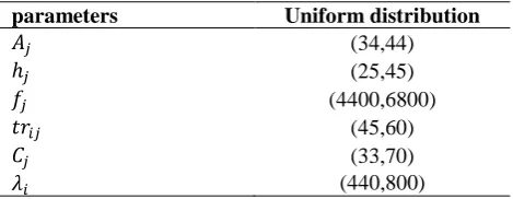
This section presents the computational results in order to test the proposed MINLP model. So, this model is coded in LINGO 9.0 software and implemented on an Intel Core i5 PC with CPU of 1.4 GHz and 4.00 GB RAM. Several test problems have been designed considering different numbers of distribution centers and retailers. The parameters in all of test problems are generated by using the Uniform distributions that are shown in Table 3. The disruption probability in all test problems is constant and equals 0.1. The computational results have been reported in Table 4.

Table 3. Distribution of parameters

parameters Uniform distribution

𝐴𝑗 (34,44)

ℎ𝑗 (25,45)

𝑓𝑗 (4400,6800)

𝑡𝑟𝑖𝑗 (45,60)

𝐶𝑗 (33,70)

Table 4. The obtained results for test problems

R = 2 R= 3

retailer*DC Best cost Execution time Best cost Execution time

4*3 64770.96 2 73953.61 3

6*4 194616.8 2 119332.1 3

9*4 285098.0 3 177395.0 3

9*5 322397.5 2 194649.7 3

9*6 288260.0 3 175944.6 3

9*7 283836.6 2 170316.0 3

13*5 411409.2 4 307518.7 3

13*6 406609.2 3 295460.2 3

13*7 413076.4 3 305239.6 5

15*5 470391.7 3 357799.2 3

20*7 718638.0 4 517219.16 4

13*13 511932.4 4 318573.1 3

4.1. Sensitivity analysis

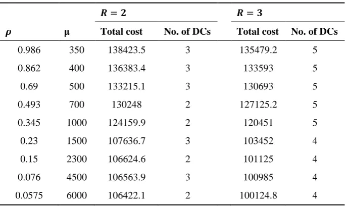
In this section, in order to illustrate the impact of some key parameters on objective function and number of distribution centers, sensitivity analysis is performed. For this work, the parameters 𝜆. 𝜇. 𝑝 and 𝑅 are changed in several levels for problems with 5 retailers and 5 distribution centers and with 6 retailers and 6 distribution centers. Tables 5 and 6 show the result of the change the value of 𝜇 for problems with 5 retailers and 5 distribution centers and with 6 retailers and 6 distribution centers, respectively. Sensitivity analyses of total costs with changing the value of 𝜇 are depicted in Figures 3 and 4 for problems with 5 retailers and 5 distribution centers and with 6 retailers and 6 distribution centers, respectively. Tables 7 and 8 show the result of the change the value of 𝜆 for problems with 5 retailers and 5 distribution centers and with 6 retailers and 6 distribution centers, respectively. Sensitivity analyses of total costs with changing the value of 𝜆 are depicted in Figures 6 and 7. Figures 5 and 8 summarize the sensitivity analyses of total costs for two problem sizes by changing the values of 𝜇 and 𝜆, respectively. Table 9 shows the results of change the value of 𝑝 and 𝑅 for problem with 5 retailers and 5 distribution centers.

Table 5. The obtained results for a problem with 5 DCs and 5 retailers

𝑹 = 𝟐 𝑹 = 𝟑

𝝆 μ Total cost No. of DCs Total cost No. of DCs

0.986 350 121077.8 3 119169 5

0.862 400 119946.5 3 117025 5

0.69 500 116312.4 3 113958 5

0.493 700 114945.41 2 110765 5

0.345 1000 109125.2 2 104709 5

0.23 1500 99713.1 3 86526 4

0.15 2300 89124.2 2 84296.7 4

0.076 4500 88857.6 3 82415.2 3

Figure 3. Sensitivity analysis of costs with changing the value of μ for a problem with 5 DCs and 5 retailers

Table 6. The obtained results for a problem with 6 DCs and 6 retailers

𝑹 = 𝟐 𝑹 = 𝟑

𝝆 μ Total cost No. of DCs Total cost No. of DCs

0.986 350 138423.5 3 135479.2 5

0.862 400 136383.4 3 133593 5

0.69 500 133215.1 3 130693 5

0.493 700 130248 2 127125.2 5

0.345 1000 124159.9 2 120451 5

0.23 1500 107636.7 3 103452 4

0.15 2300 106624.6 2 101125 4

0.076 4500 106563.9 3 100985 4

0.0575 6000 106422.1 2 100124.8 4

0 20000 40000 60000 80000 100000 120000 140000

0 1000 2000 3000 4000 5000 6000 7000

𝜇

Figure 4. Sensitivity analysis of costs with changing the value of μ for a problem with 5 DCs and 5 retailers

Figure 5. Summary on sensitivity analyses of costs with changing the value of μ for two problem sizes

0 20000 40000 60000 80000 100000 120000 140000 160000

0 1000 2000 3000

_𝜇

6*6, R=2 6*6, R=3

Tota

l

cost

0 20000 40000 60000 80000 100000 120000 140000 160000

0 1000 2000 3000

_𝜇

Table 7. The obtained results for a problem with 5 DCs and 5 retailers

𝑹 = 𝟐 𝑹 = 𝟑

𝝆 𝝀 Total cost No. of DCs Total cost No. of DCs

0.015 30 122427 2 89831.054 4

0.055 110 137275 2 96512.88 4

0.1 200 164312.06 2 110731.07 4

0.15 300 184125.15 2 124608.7 4

0.25 500 230145.85 3 150245.15 4

0.4 800 270780 3 220336.4 4

0.42 840 277799 3 255336.4 4

0.45 900 311512 3 295150 4

Figure 6. Sensitivity analysis of costs with changing the value of λ for a problem with 5 DCs and 5 retailers.

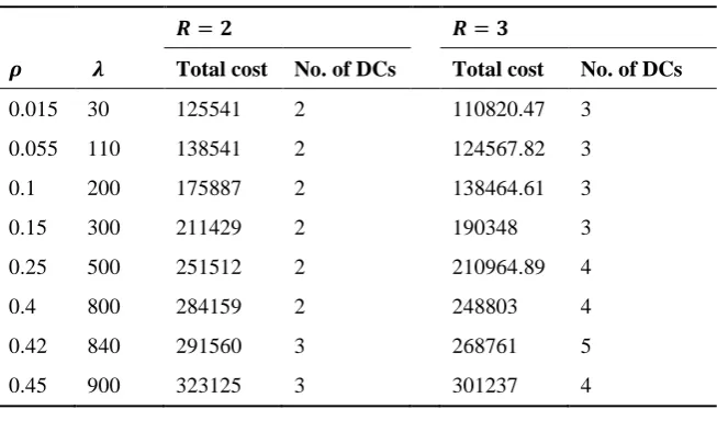
Table 8. The obtained results for a problem with 6 DCs and 6 retailers.

𝑹 = 𝟐 𝑹 = 𝟑

𝝆 𝝀 Total cost No. of DCs Total cost No. of DCs

0.015 30 125541 2 110820.47 3

0.055 110 138541 2 124567.82 3

0.1 200 175887 2 138464.61 3

0.15 300 211429 2 190348 3

0.25 500 251512 2 210964.89 4

0.4 800 284159 2 248803 4

0.42 840 291560 3 268761 5

0 50000 100000 150000 200000 250000 300000 350000

0 200 400

𝜆

Figure 7. Sensitivity analysis of costs with changing the value of λ for a problem with 5 DCs and 5 retailers.

Figure 8. Summary on sensitivity analyses of costs with changing the value of 𝝀 for two problem sizes.

0 50000 100000 150000 200000 250000 300000 350000

0 200 400 600 800 1000 1200

𝜆

6*6, R=2 6*6, R=3

0 50000 100000 150000 200000 250000 300000 350000

0 200 400 600 800 1000

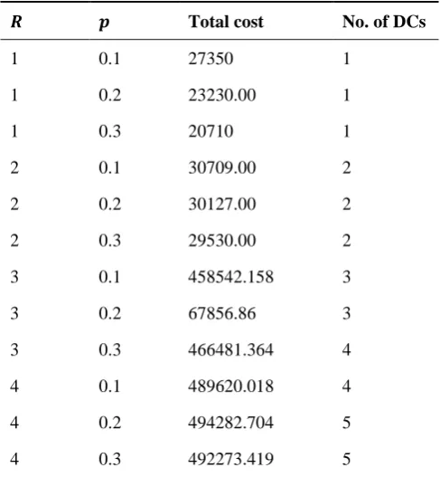
Table 9. The obtained results for a problem with 5 DCs and 5 retailers.

𝑹 𝒑 Total cost No. of DCs

1 0.1 27350 1

1 0.2 23230.00 1

1 0.3 20710 1

2 0.1 30709.00 2

2 0.2 30127.00 2

2 0.3 29530.00 2

3 0.1 458542.158 3

3 0.2 67856.86 3

3 0.3 466481.364 4

4 0.1 489620.018 4

4 0.2 494282.704 5

4 0.3 492273.419 5

According to performed sensitivity analysis, we can extract the following conclusions as well:

 By increasing the value of 𝜇, the total costs and the optimal number of DCs decrease. When the value of 𝜇 increases, expected lead time reduces and so the probability of facing shortages in each opened DC decreases. So, the mean inventory level decreases. Besides, from Constraint (15e), as the value of 𝜇 increases, the number of DCs decreases. As a result, the cost of establishing new DCs and inventory decrease.

 By increasing the value of 𝜆, the total costs and the optimal number of DCs increase. This is because when the value of 𝜆 increases, the costs of inventory and transportation will increase. Furthermore, there may be a need to establish more DCs to satisfy the retailers’ demands. Thereupon, the costs of establishing new DCs will increase.

 When 𝑅 = 1, by increasing 𝑝, the total costs increases and the optimal number of DCs decreases.

 When 𝑅 > 1, by increasing 𝑝, the total costs and the optimal number of DCs increase. That shows at a higher 𝑝, additional DCs can supply better redundancy for reliable service quality against DC failures. In fact, when retailers can be reassigned to more back-up DCs, the marginal penalty cost saving from one extra DC can better compensate the additional infrastructure investment, so making redundancy preferable.  By increasing 𝑅, the total costs and the optimal number of DCs increase.

5.

Conclusions

lead-times and also the risk of facility disruptions simultaneously in our model. The demand rate of each DC followed Poisson distribution and supplier’s lead –times was exponentially distributed. Therefore, a queuing system has been applied for calculating the mean inventory level and mean reorder rate of the steady-state condition. Then, the stochastic location- inventory problem has been formulated as a mixed integer nonlinear programming model based on the results from the queuing theory, which minimized the total expected costs of inventory, location, and transportation under all possible facility disruption scenarios. Managerial insights about model are drawn based on sensitivity analysis and numerical results. For example, when the amount of 𝜇 increases, the total costs and the optimal number of DCs will decrease, while the total costs and the optimal number of DCs increase as the value of 𝜆 increases.

For future study, the model can be developed in several directions such as, considering multi products, multi suppliers, waiting time of demand in queue and backorders. Considering facility failure probabilities as site dependence and spatial correlation.

References

Asl-Najafi, J., Zahiri, B., Bozorgi-Amiri, A., and Taheri-Moghadam, A., (2015). "A dynamic closed-loop location-inventory problem under disruption risk", Computers & Industrial Engineering, Vol. 90, pp. 414-428.

Baumol, W. J., and Wolfe, P., (1958). "A warehouse-location problem", Operations Research, Vol. 6, No. 2, pp. 252-263.

Chen, Q., Li, X., and Ouyang, Y., (2011). "Joint inventory-location problem under the risk of probabilistic facility disruptions", Transportation Research Part B: Methodological, Vol. 45, No. 7, pp. 991-1003.

Daskin, M. S., Coullard, C. R., and Shen, Z.-J. M., (2002). "An inventory-location model: Formulation, solution algorithm and computational results", Annals of operations research, Vol. 110, No. 1, pp. 83-106.

Diabat, A., Abdallah, T., and Henschel, A., (2015). "A closed-loop location-inventory problem with spare parts consideration", Computers & Operations Research, Vol. 54, pp. 245-256.

Farahani, M., Shavandi, H., and Rahmani, D., (2017). "A location-inventory model considering a strategy to mitigate disruption risk in supply chain by substitutable products", Computers & Industrial Engineering, Vol. 108, pp. 213-224.

Fontalvo, M. O., Maza, V. C., and Miranda, P., (2017). "A Meta-Heuristic Approach to a Strategic Mixed Inventory-Location Model: Formulation and Application", Transportation Research Procedia, Vol. 25, pp. 729-746.

Ghafour, K., Ramli, R., and Zaibidi, N. Z., (2017). "Developing a M/G/C-FCFS queueing model with continuous review (R, Q) inventory system policy in a cement industry", Journal of Intelligent & Fuzzy Systems, Vol. 32, No. 6, pp. 4059-4068.

Gzara, F., Nematollahi, E., and Dasci, A., (2014). "Linear location-inventory models for service parts logistics network design", Computers & Industrial Engineering, Vol. 69, pp. 53-63.

Isotupa, K. S., (2006). "An (s, Q) Markovian inventory system with lost sales and two demand classes", Mathematical and computer modelling, Vol. 43, No. 7, pp. 687-694.

Javid, A. A., and Azad, N., (2010). "Incorporating location, routing and inventory decisions in supply chain network design", Transportation Research Part E: Logistics and Transportation Review, Vol. 46, No. 5, pp. 582-597.

Kim, E., (2005). "Optimal inventory replenishment policy for a queueing system with finite waiting room capacity", European journal of operational research, Vol. 161, No. 1, pp. 256-274.

Krishnamoorthy, A., Shajin, D., & Lakshmy, B., (2016). "On a queueing-inventory with reservation, cancellation, common life time and retrial". Annals of operations research, Vol. 247, No. 1, pp. 365-389.

Liao, S.-H., Hsieh, C.-L., and Lai, P.-J., (2011). "An evolutionary approach for multi-objective optimization of the integrated location–inventory distribution network problem in vendor-managed inventory". Expert Systems with Applications, Vol. 38, No. 6, pp. 6768-6776.

Lin, J.-R., Yang, T.-H., and Chang, Y.-C., (2013). "A hub location inventory model for bicycle sharing system design: Formulation and solution", Computers & Industrial Engineering, Vol. 65, No. 1, pp. 77-86.

Liu, L., Liu, X., and Yao, D. D., (2004). "Analysis and optimization of a multistage inventory-queue system". Management Science, Vol. 50, No. 3, pp. 365-380.

Macchion, L., Danese, P., and Vinelli, A., (2015). "Redefining supply network strategies to face changing environments. A study from the fashion and luxury industry", Operations management research, Vol. 8, pp. 15-31.

Melikov, A., and Shahmaliyev, M., (2017). "Analysis of Perishable Queueing-Inventory System with Positive Service Time and (S-1, S) Replenishment Policy", Paper presented at the International Conference on Information Technologies and Mathematical Modelling.

Miranda, P. A., and Garrido, R. A., (2004). "Incorporating inventory control decisions into a strategic distribution network design model with stochastic demand", Transportation Research Part E: Logistics and Transportation Review, Vol. 40, No. 3, pp. 183-207.

Miranda, P. A., and Garrido, R. A., (2008). "Valid inequalities for Lagrangian relaxation in an inventory location problem with stochastic capacity", Transportation Research Part E: Logistics and Transportation Review, Vol. 44, No. 1, pp. 47-65.

Qu, H., Wang, L., and Liu, R., (2015). "A contrastive study of the stochastic location-inventory problem with joint replenishment and independent replenishment", Expert Systems with Applications, Vol. 42, No. 4, pp. 2061-2072.

Ramezani, M., (2014). "A quoining-location model for in multi-product supply chain with lead time under uncertainty".

Sadjadi, S. J., Makui, A., Dehghani, E., and Pour Mohammad, M., (2016). "Applying queuing approach for a stochastic location-inventory problem with two different mean inventory considerations", Applied Mathematical Modelling, Vol. 40, No. 1, pp. 578-596.

Saffari, M., and Haji, R., (2009). "Queueing system with inventory for two-echelon supply chain", Paper presented at the Computers & Industrial Engineering, 2009. CIE 2009. International Conference.

Schwarz, M., and Daduna, H., (2006). "Queueing systems with inventory management with random lead times and with backordering", Mathematical Methods of Operations Research, Vol. 64, No. 3, pp. 383-414.

Shen, Z.-J. M., Coullard, C., and Daskin, M. S., (2003). "A joint location-inventory model", Transportation science, Vol. 37, No. 1, pp. 40-55.

Teimoury, E., Modarres, M., Ghasemzadeh, F., and Fathi, M., (2010). "A queueing approach to production-inventory planning for supply chain with uncertain demands: Case study of PAKSHOO

Chemicals Company", Journal of Manufacturing Systems, Vol. 29, No. 2, pp. 55-62.

Zeng, J., Phan, C. A., and Matsui, Y., (2013). "Supply chain quality management practices and performance: An empirical study", Operations management research, Vol. 6, pp. 19-31.

Zhang, Z.-H., and Unnikrishnan, A., (2016). "A coordinated location-inventory problem in closed-loop supply chain". Transportation Research Part B: Methodological, Vol. 89, pp. 127-148.