A knowledge-based NSGA-II approach for scheduling in virtual manufacturing cells

JIEMS

Journal of Industrial Engineering and Management Studies

Vol. 3, No. 1, pp. 89 - 107

www.jiems.icms.ac.ir

A knowledge-based NSGA-II approach for scheduling in virtual

manufacturing cells

M. Zandieh1,* Abstract

This paper considers the job scheduling problem in virtual manufacturing cells (VMCs) with the goal of minimizing two objectives namely, makespan and total travelling distance. To solve this problem two algorithms are proposed: traditional non-dominated sorting genetic algorithm (NSGA-II) and knowledge-based non-dominated sorting genetic algorithm (KBNSGA-II). The difference between these algorithms is that, KBNSGA-II has an additional learning module. Finally, we draw an analogy between the results obtained from algorithms applied to various test problems. The superiority of our KBNSGA-II, based on set coverage and mean ideal distance metrics, is inferred from results.

Keywords: Multi-objective optimization; Non-dominated sorting genetic algorithm; Knowledge based algorithm; Virtual manufacturing cells; Job scheduling.

Received: Oct2016-24

Revised: Dec2016-20

Accepted: Dec2016-20

1. Introduction

For most enterprises, it is of vital importance that the manufacturing processes to be optimally controlled. That is, to minimize manufacturing cost, satisfy the production schedule and to improve productivity. In some industries the optimal control of the system is a complex and hard task to carry out. Typically these companies specialize in a few processes and render their production facilities for the manufacturing of a variety of parts. A well-known method for improving planning and control in such industries is virtual manufacturing cells (VMCs). The virtual cell concept was first developed at the national bureau of standards as part of the control software for the automated manufacturing research facility (AMRF) project. A virtual cell is a logical grouping of workstations

* Corresponding Author.

1

which are dynamically generated and controlled and are not necessarily transposed into physical proximity (McLean et al., 1982). The grouping is based on a predefined logic and only exists in the production control system and in the minds of the workers. Virtual manufacturing cells are created periodically, for instance every week or every month depending on changes in volumes and mix of demand (Slomp et al., 2005). A virtual cell controller takes over the control and identifies a set of required machines with spare capacity to process the jobs. In VMC a machine can be shared among several cells. This increases the performance of cells.

A new approach for layout in VMCs is scattered layout. This approach was first suggested by Montreuil et al. (1991), in which to increase accessibility, similar machines are scattered across the shop floor. Since the similar machines are not located in close proximity travelling distance between machines must be considered when scheduling jobs. Nomden et al. (2006) have surveyed an excellent taxonomy of past research devoted entirely to VMCs. We provide state of the art related to VMCs as follows.

Kesen et al. (2009) investigated the three different types of layouts namely cellular, process and virtual cells. They compared the performance of these layouts using simulation technique. They developed an ant colony optimization to reveal the behavioral characteristics of each layout. Kesen et al. (2010) presented a multi objective mixed integer programming formulation for job scheduling in VMCs, where the objective is to minimize the sum of the weighted makespan and total travelling distance. They also developed a genetic algorithm based on heuristic for scheduling of jobs in VMCs.

In this paper we employed two objective meta-heuristic algorithms for solving the multi-objective mixed integer programming formulation which Kesen et al. (2010) have presented. First, we applied a non-dominated sorting genetic algorithm II (NSGA-II) and then a new algorithm called knowledge based non-dominated sorting genetic algorithm (KBNSGA-II) to solve Kesen’s formulation. Both algorithms were tested on various problems and the results were compared using various comparison metrics.

This paper is organized as follows: In Section 2 we present the problem description with the assumptions and mathematical formulation. Section 3 introduces non-dominated sorting genetic algorithm for VMCs scheduling. A knowledge-based sorting genetic algorithm is presented in Section 4. Section 5 presents experimental results and comparison of the proposed algorithms in term of some metrics. Finally, Section 6 states our conclusions and future researches on this topic.

2. Problem description and formulation

This paper is concerned with the scheduling of jobs in VMCs where there are n jobs and m

machine types. Each machine type can include at least two machines. ( )s i is an individual machine that is a member of machine type i s i





operation of job j. Each job has its specific route and the machines that can process O_{j h,} are predefined. If Oj h, is performed in machine type i, all s i( ) machines compete to perform the

The problem consists of two parts: machine assignment and scheduling. Each job can only visit each machines once. Jobs are produced in batches. Processing times, batch sizes as well as precedence relationships are defined in advance. Batch splitting is not permissible, i.e. when O_{j h,} is allocated to machine s i( ) all operations in the batch must be performed on that machine. Moreover, when O_{j h,} starts all operations in the batch must be completed without interruption and preemption. All jobs are available at time zero. Machines are stationary and distances between each pair of machine are predefined. Breakdown and maintenance activities are ignored. . The notations for the problem definition and formulation are given as follow (Kesen et al. 2010).

Parameters

j job index (j1, 2,..., )n

,

i k machine group index ( ,i k1, 2,..., )m

l index for order on each machine (l1, 2,...,l_{s i( )}) h operation index (h1, 2,...,h_j)

, j h

O hth operation of job j

( )

s i individual machine s belonging to machine group i

j

N batch size of job j

jh

P unit processing time of operation h of job j

( ), ( ) s j s k

D unit transportation cost for each job from machine s i( ) to s k( )

M very big number q

w weight of the qth objective function Decision variables

max

C makespan or completion time of all jobs ( ), ,

s i j h

Y 1 if machine s i( ) is selected for operation O_{j h,} , 0 otherwise

( ), , , s i j h l

X 1 if O_{j h,} is performed on machine ( )s i in the order l, 0 otherwise

, j h

t starting time of operation O_{j h,} ( ),

s i l

Tm starting time of the machine ( )s i for the order l

max ( ), , ( ), , 1 ( ), ( )

1 1 1 1

min , (1)

j

h

n m m

s i j h s k j h s i s k j j h i k

C Y Y D N

   

 

 

 





Subject to:

max j h, j h, j; 1, 2,..., ; 1, 2,..., j (2)

C t P N j n h h

, , , 1; 1, 2,..., ; 1, 2,..., 1 (3)

j h j h j j h j

t P N t  j n h h 

( ), ( ), , , , ( ), 1; 1, 2,..., ; 1, 2,..., ; 1, 2,..., ; 1, 2,..., ( ) 1 (4)

s i l s i j h l j h j s i l j s i

Tm X P N Tm  i m j n h h l l 

, .(1 ( ), , , ) ( ), ; 1, 2,..., ; 1, 2,..., ; 1, 2,..., ; 1, 2,..., ( ) (5)

j h s i j h l s i l j s i

t M X Tm i m j n h h l l

( ), .(1 ( ), , , ) , ; 1, 2,..., ; 1, 2,..., ; 1, 2,..., ; 1, 2,..., ( ) (6)

s i l s i j h l j h j s i

( ), , , ( ) 1 1

1; 1, 2,..., ; 1, 2,..., (7)

j

h n

s i j h l s i

j h

X i m l l

 

  



( ), , 1; 1, 2,..., ; 1, 2,..., (8)

s i j h j

i

Y  j n h h



( ), , , ( ), , ; 1, 2,..., ; 1, 2,..., ; 1, 2,..., (9)

s i j h l s i j h j

l

X Y i m j n h h



max 0; j h, 0; s i l( ), 0; s i( ), , ,j h l, s i( ), ,j h {0, 1} (10)

C  t  Tm  X Y 

The objective function in equation (1) minimizes the total travelling distance and the completion time of all jobs. Constraints in equation (2) assure that makespan must be greater than or equal to the completion times of all operations. The constraints in equation (3) secure that no operation can be started unless the preceding operations have been completed. The constraints in equation (4) indicate that successive operations of any machine must wait for the preceding operation to be completed. Constraint sets (5) and (6) enforce that if X_{s i( ), , ,j h l} is equal to 1 the hth operation of job j and the lth order on machine s i( ) must start at the same time. Constraint (7) shows that only one operation can be assigned on each order of operation on any machine. Equation (8) indicates that every operation is assigned only to one machine. Equation (9) ensures that if an operation is assigned to any particular machine, this operation will be positioned only once. Constraint set (10) enforces that decision variable must be greater than or equal to zero.

3. A NSGA-II for the job scheduling in VMCs problem

Finding the global optimum for a general multi objective optimization problem (MOOP) is NP-Complete (Back, 1996). In a MOOP, finding a solution that optimizes all objectives is ideal but because of conflicting objectives, in most cases, a set of solutions is found. Consider a general multi-objective minimization problem with p decision variables and q objectives (q1):

Minimize y f x( )( ( ),f x₁ f x₂( ),...,f x_q( )) Subject to:

x( ,x x_{1 2},...,x_p)X y( ,y y_{1 2},...,y_q)Y

Where x is the decision vector, y is the objective vector, X is the parameter space and Y is the objective space. We say solution a dominate solution b, if and only if: f ai( ) f bi( ); i {1,..., }q and f ai( ) f bi( ); i {1,..., }q . Non-dominated solutions are a set of solutions that dominate the others but do not dominate themselves. A feasible solution which is not dominated by any other solution in all feasible space is called Pareto optimal. The Pareto optimal set, which is also called the efficient set, is the collection of all Pareto optimal solutions. Pareto optimal solutions in the objective space are called the Pareto optimal frontier.

comparison mechanism, genetic operators and an elitist approach. The NSGA-II ranks each solution based on dominance. The solutions of the current population are partitioned in non-dominated fronts. The first non-dominated front contains all non-dominated solutions in the population. The second non-dominated front contains all non-dominated solutions obtained after removing the first front. This process continues till all solutions are fitted in a front. The NSGA-II also calculates the crowding distance for each individual solution. Crowding distance gives the algorithm the ability to distinguish individual solutions that are in the same frontier. The individual solutions that are in a lower frontier are considered better than those in higher frontier. If the individual solutions are in the same frontier, then those that have upper crowding distance are considered better.

if (i 1) m

f  and (i 1) m

f  denote the values for objective function m for the nearest solution surrounding solution i with (i 1) i (i 1)

m m m

f   f  f  , max m

f and min m

f the maximum and the minimum values for objective function m and M is the total number of objective, then crowding distance ( )d_i for a solution i is calculated by

( 1) ( 1) max min 1

i i

M

m m

i

m m m

f f

d

f f

 



 





NSGA-II starts with the creation of a random population of solutions P₀ of size N, where N is the population size. Solutions are ranked using the concept of non-dominated sorting. A new population of solutions Q₀ is created using the set of recombination operators that are appropriate for the problem considered. The old and the new generation of solutions are merged into a new population of solutions R_t of size 2N . Non-dominated sorting is subsequently used to sort the solutions contained in R_t. According to the ranking priorities, fronts from the combined population (R_t) are moved to intermediate population P_t1. If the last move would not fill the P_t1 completely and the next move is bigger than the size of space left in P_t1 then based on crowding distance the best solution from last front are moved to P_t₁. The new population of solutions Qt1 is created from Pt1

through the typical recombination operators. The same process is repeated for a pre-specified number of generations. The specially designed components of the proposed NSGA-II are explained in following sections:

3.1. The representation mechanism and the schedule generation scheme

There are two parts to each solution (chromosome). One represents operation sequence vector and the other machine assignment vector. Elements in the first vector indicate the order of operations related to jobs and elements in the second vector represents the selected machine for the corresponding operation. To show the inner working of thisrepresentation mechanism Consider the case where there are three types of machines, namely A, B and C and each machine type has four, two and two machines respectively. Furthermore, there are four jobs namely 1, 2, 3 and 4 that consist of three, two, two and two operations respectively (see Table 1 and 2). For this case, one possible schedule could be (O4,1O2,1O4,2O1,1O1,2 O3,1O1,3 O2,2 O3,2), where

ij

job index (see Figure 1). To decode the solutions in the new representation, reading the data from left to right, for each occurrence of the job index, the operation index is increased by one.

4 2 4 1 1 3 1 2 3

o

o

o

o

o

o

o

o

o

Figure 1: Operation order vector

Machine selection vector is presented using an array of values. For the problem shown in Table 1 and 2 one possible encoding of the machine selection vector is presented in Figure 2. This solution representation is derived from representation of Gen et al. (1994).

o

o

o

o

o

5 3 8 7 1 5 8 2 6

o

o

o

Operation

Machine selection

o

Figure 2: Machine selection vector

Table 1: Machine types and individual machines belonging to it

Machine type Machine number A 1, 2, 3, 4 B 5, 6 C 7,8

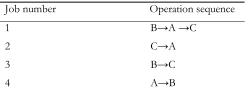
Table 2: Operation sequences for the jobs

Job number Operation sequence 1 B→A →C

2 C→A

3 B→C

In this paper, only active schedules are considered. An active schedule is defined as a feasible schedule, where no operation can be started earlier unless at least one other operation is delayed or some constraints are violated. In order to generate an active schedule, each operation is allocated to its predetermined machine in the order identified in the operation sequence vector. When operation

jh

O is scheduled on machine s i( ) the blank intervals between operations that have already been scheduled on machine s i( ) are evaluated from left to right to detect the earliest feasible time available. If such a time interval is found, it will be allocated there. Otherwise it will be allocated at the end of scheduled operations.

3.2. Selection strategy

The selection strategy chooses a number of chromosomes as parents to implement the genetic operators on them. In this research, a crowded tournament selection operator with tour-size=2 is used. In the crowded tournament selection, first we select two chromosomes to attend the tournament randomly. If the two chromosomes are in the different frontiers, then the chromosome with the best frontier would be selected as winner. Otherwise the chromosome with the best crowding distance is selected.

3.3. Crossover operators

In this paper, two crossover operators are employed to create an offspring. One of them is to create the operation sequence part of child and the other to create the machine assignment part of child. These operators are defined as follows:

Crossover operator for operation sequence vector:In the proposed solution representation, there are similar numbers in the operation sequence vector but each number represents a different concept. This makes it difficult to define the crossover operator. To overcome this, the representation for operation sequence vector is transformed into the permutation representation.

In order to implement permutation representation all operations are assigned a fixed ID as shown in Figure 3. Then all operations in the operation sequence vector are shown with their respective ID number. For instance, permutation representation for operation sequence in Figure 1 can be represented as shown in Figure 4.

o

o

o

o

o

1 2 3 4 5 6 7 8 9

o

o

o

Operation

Fixed ID

o

Figure 3: Fixed ID for each operation

o

o

o

o

o

8 4 9 1 2 6 3 5 7

o

o

o

Operation reffered

Operation sequence

o

The crossover operation is implemented as follows: First, we randomly select a substring of operation sequence vector from first parent. Next we produce a proto child by copying this substring into the corresponding positions in child. The corresponding operations of substring are deleted from the second parent. Finally, the remaining operations in the second parent are placed into the unfilled positions of the proto-child from left to right. After the crossover operator is implemented, the offspring in the operation sequence vector are converted into the prior representation and a feasible child is produced. This procedure has been proposed by Gao et al. (2004). An example of this crossover is illustrated in Figure 5.

8 4 9 1 2 6 3 5 7

Parent 1

4 8 5 1 2 6 3 9 7

Parent 2

4 8 9 1 2 5 6 3 7

Offspring

Figure 5: Order crossover on operation sequence vector

Crossover operator for machine assignment vector: the operation sequence vector of an offspring is produced by a Uniform crossover operator. Uniform crossover first generates a random crossover mask and then exchanges relative genes between parents according to the mask. A crossover mask is a binary string randomly generated and equal in size to the chromosomes. The mask is scanned from left to right. If the current bit is 1 then the child inherits the corresponding gene from first parent. Otherwise the genes are supplied from the second parent. The second offspring is produced in the similar way, except that when current position is 1 in the string the genes are selected from the second parent and when 0 the selection is from the first parent. It is illustrated in Figure 6.

5 4 3 6 3 7 4 4 2 6

6 2 1 4 6 2 5 6 3 7

1 0 0 1 0 1 1 0 1 0

6 4 3 4 3 2 5 4 3 6

5 2 1 6 6 7 4 6 2 7

Parent 1

Parent 2

Mask

Offspring 1

Offspring 2

3.4. Mutation operator

Mutation operator is implemented in both the operation sequence vector and the machine assignment vector, separately.

Mutation operator for machine assignment vector: An operation is selected randomly and from among the machines can process this operation, one is selected randomly and replaces previous machine.

Crossover operator for operation sequence vector: To mutate in operation sequence an operation is selected randomly and its position in the operation sequence vector is swapped with the position of its immediate prior operation.

4. The proposed knowledge based NSGA-II

4.1. Introduction

In recent years the study of interaction between evolution and learning in combinational optimization problems has been attracting much attention and several research have been done in this field (e.g. by Ho et al. (2007), Chung and Reynolds (1996), Branke (1999), Louis and McDonnell (2004), Michalski (2000), Xing et al. (2010)). The diversity of these methods and their positive results has persuaded us to opt for a holistic architecture called knowledge-based heuristic searching (KBHSA). KBHSA comprises the integration of two modules namely knowledge and heuristic search. Heuristic searching module searches through the wide solution space and finds good solutions. The knowledge module learns the available knowledge from the same good solutions and feeds it back to heuristic searching module. We demonstrate the performance of this architecture in a new algorithm called knowledge based non-dominated sorting genetic algorithm (KBNSGA-II). The general idea for this methods is to keep good and/or bad features of the previous solutions to improve the quality of next solutions. We use operational memory (OM) to save good features of previous solutions which initially was proposed by Ho et al. (2007) for flexible job-shop schedules in the algorithm named LEGA.

4.2. Operational memory

Operational memory is an array of bits that contains the set of suitable machines for generating improved solutions (see Figure 7).

1 1 0 0 1 0 1 1 1 0 1 0 1 0 1 1 1 0 0 0 1 1 1 1

M5 M6

o

M1

o

o

M3 M4

o

M7 M8

o

o

M2 M1 M2

o

M3M4 M5

o

M6

o

M1 M2 M3 M4 M5 M6 M7 M8

M7 M8

Figure 7: Operational memory

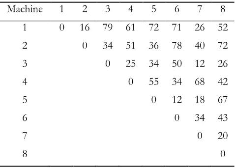
(i) OM initialization: In initializing OM we must consider two objectives, the makespan and the total traveling distance. We were able to extract the initial knowledge for the total traveling distance but the useful initial knowledge for minimizing the total completion time of the jobs was not attained. Initial knowledge for minimizing the total traveling distance of jobs is explained below. Every job can choose different routes between machines for its completion. All possible routes for that job are evaluated and k number of best routes are discovered and OM is initialized by them (k is the number of operations related to that job). For instance, consider the problem shown by Table 1, 2 and 3. Table 3 shows the distance between machines. Job 1 in Table 2 consists of three operations namely O_1,1,O_1,2,O_1,3 which have to be processed by machine types B, A and C. According to Table 1, each machine types B, A and C consist of 2, 4 and 2 machines respectively. Therefore, Job 1 has 16 (2 4 2 16)   routes to choose from. Using Table 3 the following three shortest routes are chosen.

M5→M3→M7 TTD=46 M5→ M3→M8 TTD=60 M6→ M3→M7 TTD=62

According to these three routes, machines M5 and M6 are suitable for operation O1,1. Therefore bits

related to machines M5 and M6 in OM for operation O1,1 is set to 1. The machine that is considered

for operation O_1,2 is M3. Similarly, machines M7 and M8 deemed suitable for operation O1,3. The bit

related to machine M3 for operation O1,2 and the bits related to machine M7 and M8 for operation 1,3

O are set to 1. The rest of the bits related to operations of Job 1 remain at zero. Likewise suitable routes for all jobs are identified and OM is initialized. Figure 7 depicts an initialized OM for the given example.

(ii) Updating of OM: With the repetition of algorithm, it is possible to discover other suitable machines and OM would be updated. In each generation all solutions in first front are used for updating OM and consequently the number of bits that have the value of 1 would increase.

Table 3. Distance matrix between each pair of machine

Machine 1 2 3 4 5 6 7 8 1 0 16 79 61 72 71 26 52 2 0 34 51 36 78 40 72 3 0 25 34 50 12 26

4 0 55 34 68 42

5 0 12 18 67

6 0 34 43

7 0 20

4.3. Applying OM on the proposed KBNSGA-II

The difference between KBNSGA-II and NSGA-II is that KBNSGA-II has an additional mutation operator named intelligent mutation. In intelligent mutation when selecting a new machine for an operation, suitable machines are selected from OM. The steps of intelligent mutation operator in machine selection vector are presented below.

1) Select an operation O_ij randomly from operation sequence vector of a solution 2) Detect machine M_k that is currently selected to process O_ij.

3) Detect a set of machines (P O_ij) that can process O_ij

4) Identify a set of suitable machines POM O( _ij) in Operational Memory that can process O_ij

5) If POM O( _ij) contains only M_k then select a machine randomly from (P O_ij). Otherwise, select a random machine in POM O( _ij) (except M_k) to process O_ij.

5. Experimental design

5.1. Test problems

Thirty nine test problems were created to examine the performance of the algorithms. Data required for a problem are the distance between each pair of machines, processing time of jobs on machines and batch size. Distances between each pair of machines in the test problem are uniformly distributed from 10 to 80. Processing time of jobs on machines follows the uniform distribution with a lower bound of 2 and upper bound of 10. Batch size also corresponds to uniform distribution with a lower bound of 5 and upper bound of 40.

5.2. Evaluation metrics

To evaluate the effectiveness and performance of the proposed algorithms the following five comparison metrics are considered:

(1) Spacing metric: This metric measures the uniformity of the spread of the points of the solution set. It is defined as follows:

2

1

1

( )

Q

i i

S d d

Q 





where

, 1

min M

i k

i m m

k Q k i m

d f f

  _





1 Q

i

i

d d

Q







the number of non-dominated solution in ,Q M is the number of objectives and f_ji is the value of objective function j for solution i. The lower value of spacing metric the better solution quality we have.

{ | : } ( , ) b B a A a b C A B

B

  



(3) Mean ideal distance (MID): This metric shows the closeness between Pareto solution and ideal point (0,0). Lower values of MID are preferred.

1 Q

i i

D MID

Q







1 2

( i) ( i) ... ( i )

i M

D  f  f   f

(4) Maximum spread metric: this metric measures the Euclidean distance between boundary objectives values in the non-dominated solutions. The higher value of set coverage metric, the better solution quality we have.

2

1 1

1

(max min )

Q Q

M

i i

m m

i i

m

D f f

 







(5) The number of Pareto solutions: This metric shows the number of Pareto solutions that each algorithm obtain. We have the better solution quality, whenever this metric is higher.

5.3. Experimental results

The algorithms were coded in Borland C++ and executed on a computer with 2.1 GHz Intel Core 2 Duo processor and 2GB of RAM. We executed the algorithms 3 times for each problem. The computational time for the problems 1 to 18 and 19 to 39 are determined to be 60 and 180 seconds, respectively. The population size for both algorithms ranges from 300 to 5000 Depending on the complexity of the problems. Crossover probability is 0.7. Mutation probability in NSGA-II is 0.3. Intelligent and simple mutations in KBNSGA-II are set at 0.24 and 0.06 respectively.

In this paper RPD is applied as a common performance measure to compare the algorithms (Ruiz and Allahverdi, 2007). RPD for spacing and mean ideal distance metrics is calculated by the following formula:

100 Sol LB RPD

LB



 

Where, sol is the objective function value obtained from a given algorithm for each instances of its execution. LB is the best solution obtained from both algorithms. RPD For maximum spread and the number of Pareto solution metrics is calculate as follow:

100 UB Sol RPD

UB



 

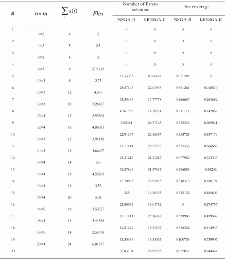
# : problem number :

n number of jobs :

m number of machine types :

Flex average number of equivalent machines per operation

Table 4. RPD values of the number of Pareto solutions and values of set coverage metric for algorithms.

Set coverage Number of Pareto

solutions Flex ( ) i s i



n m

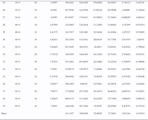
Table 5. RPD values of Spacing, Maximum spread and MID metrics for the algorithms MID Maximum spread Spacing Flex ( ) i s i



n m

1.636741 1.110642 1.680163 0.076514 2.935825 1.46918 1.798964 2.952191 4.198806 2.656749 1.304348 3.106266 3.145251 3.088123 4.153152 1.670314 2.736112 2.86889 0.882059 1.547209 1.527537 1.811919 2.223352 2.352625 5.785695 3.612942 2.551022 4.237655 4.089312 5.889459 4.305791 2.421164 44.18387 25.02028 51.70065 13.48464 41.41806 35.77596 33.84191 10.76106 75.32104 44.55521 32.30925 50.25078 44.40162 72.77698 42.69404 27.2684 59.84582 67.80154 81.99853 11.11885 52.94436 28.85419 42.2813 66.15424 44.18482 71.08444 75.06103 35.94961 29.16576 36.63923 69.8149 32.48029 926.9429 162.9596 1734.811 126.2618 122.1881 115.5011 502.9213 1662.493 89.24439 158.4972 1263.631 1009.05 237.1833 131.4423 967.1466 328.6058 309.4261 82.79936 85.39437 235.8405 216.7817 503.1054 207.4439 236.6583 191.3561 19.89574 300.4056 398.2369 173.0098 800.9179 144.6526 161.5357 5.0099 8.0381 4.4589 4.47009 8.41379 4.62411 5.83459 5.72152 7.47651 5.9021 9.13194 5.98477 7.96571 5.63819 7.0625 20 32 26 18 32 18 24 28 38 24 36 30 40 34 42 35×4 35×4 35×6 40×4 40×4 45×4 45×4 45×5 45×5 50×4 50×4 50×5 50×5 50×6 50×6 25 26 27 28 29 30 31 32 33 34 35 36 37 38 39 Mean

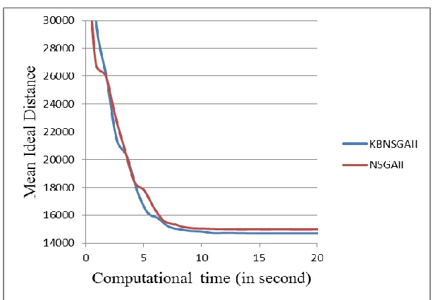
To compare the two algorithms in term of the five metrics, the two sample ttests are performed and the results are shown in Tables 6-10. The results indicate that KBNSGA-II is preferred with respect to the set coverage and the mean ideal distance metrics. Moreover, in spacing metric the obtained results from NSGA-II are better than those of KBNSGA-II. This is because the knowledge module (OM) guides the algorithms toward promising space and therefore the search space is condensed. However, since NSGA-II searches a larger space, metrics related to diversity obtained from NSGA-II are preferred. Figure 8 depicts the convergence of both algorithms in minimizing the mean ideal distance metric for Problem 21.

N Mean StDev SE Mean NSGA-II 39 25.6 18.1 2.9 KBNSGA-II 39 26.2 17.5 2.8 Difference = mu NSGA-II - mu KBNSGA-II Estimate for difference: -0.65

95% upper bound for difference: 6.06

t-test of difference = 0 (vs <): t-value = -0.16 p-value = 0.436 df = 75

Table 7. Two-sample ttest for NSGA-II vs KBNSGA-II in term of set coverage

N Mean StDev SE Mean NSGA-II 39 0.262 0.220 0.035 KBNSGA-II 39 0.457 0.307 0.049 Difference = mu NSGA-II - mu KBNSGA-II Estimate for difference: -0.1954

95% upper bound for difference: -0.0944

t-test of difference = 0 (vs <): t-value = -3.23 p-value = 0.001 df = 68

Table 8. Two-sample ttest for NSGA-II vs KBNSGA-II in term of spacing

N Mean StDev SE Mean NSGA-II 39 162 170 27 KBNSGA-II 39 329 494 79 Difference = mu NSGA-II - mu KBNSGA-II Estimate for difference: -167.1

95% upper bound for difference: -26.8

t-test of difference = 0 (vs <): t-value = -2.00 p-value = 0.026 df = 46

Table 9. Two-sample ttest for NSGA-II vs KBNSGA-II in term of maximum spread

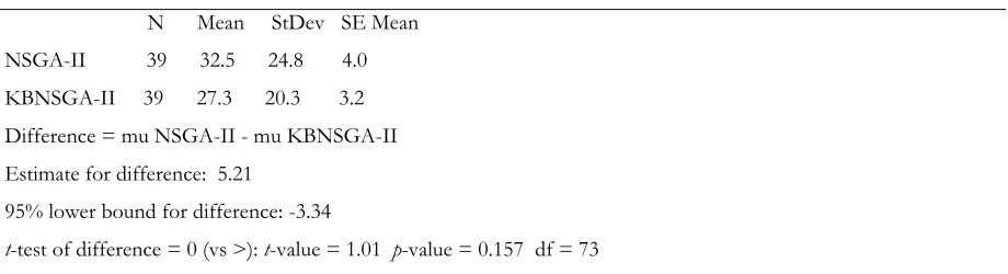
N Mean StDev SE Mean NSGA-II 39 32.5 24.8 4.0 KBNSGA-II 39 27.3 20.3 3.2 Difference = mu NSGA-II - mu KBNSGA-II Estimate for difference: 5.21

95% lower bound for difference: -3.34

Table 10. Two-sample ttest for NSGA-II vs KBNSGA-II in term of mean ideal distance

N Mean StDev SE Mean NSGA-II 39 2.42 1.94 0.31 KBNSGA-II 39 1.67 1.24 0.20 Difference = mu NSGA-II - mu KBNSGA-II Estimate for difference: 0.751

95% lower bound for difference: 0.134

t-test of difference = 0 (vs >): t-value = 2.03 p-value = 0.023 df = 64

Figure 8: Convergence of proposed algorithms in minimizing the MID metric

6. Conclusion

Further research can concentrate on developing the proposed knowledge-based procedure for other scheduling problems or applying the learning method in other meta-heuristics. Another future research may be the consideration of some other realistic assumptions such as machine availability constraints, batch splitting and sequence-dependent setup times. To add the other optimization objectives in the problem such as minimization of maximum machine workloads is another opportunity for research.

References

Back, T., 1996. Evolutionary Algorithms in Theory and Practice, Oxford University Press: New York, NY. Branke, J., 1999. Memory-enhanced evolutionary algorithms for dynamic optimization problems. Proceedings of the Congress on Evolutionary Computation, IEEE Press, Piscataway, 1875-1882.

Louis, S.J., McDonnell, J., 2004. Learning with case-injected genetic algorithms. IEEE Transactions on Evolutionary Computation 8(4).

Chung, C.J., Reynolds, R.G., 1996. A test-bed for solving optimization problems using cultural algorithm, in: Proceedings of the Fifth Annual Conference on Evolutionary Programming, MIT Press, Cambridge, 225-236. Deb, K., Pratap, A., Agarwal, S., Meyarivan, T., 2002. A fast and elitist multi-objective genetic algorithm: NSGA-II. IEEE Trans Evolutionary Comput. 6, 182–197.

Gao, J., Sun, L., Gen, M., 2008. A hybrid genetic and variable neighborhood descent algorithm for flexible job shop scheduling problems. Computers and Operations Research 35(9), 2892-2907.

Ho, N.B., Tay, J.C., Lai, E.M.K., 2007. An effective architecture for learning and evolving flexible job-shop schedules. European Journal of Operational Research 179(2), 316-333.

Kesen, S.E., Toksari, M.D., Gungor, Z., Guner, E., 2009. Analyzing the behaviors of virtual cells (VCs) and traditional manufacturing systems: Ant colony optimization (ACO)- based metamodels. Computers & Operations Research 36(7), 2275-2285.

Kesen, S.E., Das, S.K., Gungor, Z., 2010. A genetic algorithm based heuristic for scheduling of virtual manufacturing cells (VMCs). Computers and Operations Research 37, 1148-1156.

McLean, C.R., Bloom, H.M., Hopp T.H., 1982. The virtual manufacturing cell. In: Proceedings of the fourth IFAC/IFIP conference on information control problems in manufacturing technology, Gaithersburg, MD, 1– 9.

Michalski, R.S., 2000. Learnable evolution model: evolution process guided by machine learning. Machine Learning 38(1), 9-40.

Nomden, G., Slomp, J., Suresh, N.C., 2006. Virtual manufacturing cells: A taxonomy of past research and identification of future research issues. International Journal of Flexible Manufacturing System 17, 71-92. Montreuil, B., Venkatadri, U., Lefrancois, P., 1991. Holographic layout of manufacturing systems. 19th HE Systems Integration Conference, 1-13.

Ruiz, R., Allahverdi, A., 2007. Some effective heuristics for no-wait flow-shops with setup times to minimize total completion time. Annals of Operations Research 156, 143-171.

Srinivas, N., & Deb, K., 1994. Multi-objective function optimization using nondominated sorting genetic algorithms. Evolutionary Computation Journal 2(3),221-248.

Gen, M., Tsujimura, Y., Kubota E., 1994. Solving job-shop scheduling problem using genetic algorithms. In: Proceedings of the 16th international conference on computer and industrial engineering, Ashikaga, Japan, 576–9.

Slomp, J., Chowdary, B.V., Suresh, N.C., 2005. Design of virtual manufacturing cells: a mathematical programming approach, Robotics and Computer-Integrated Manufacturing 21, 273–288.