MODIFIED GENETIC ALGORITHM BASED SOFTWARE RELIABILITY USING SPRT: RAYLEIGH MODEL

Http://www.ijetmr.com©International Journal of Engineering Technologies and Management Research [17]

MODIFIED GENETIC ALGORITHM BASED SOFTWARE RELIABILITY

USING SPRT: RAYLEIGH MODEL

Dr. R.Satyaprasad1_{, Ch.Surya Kiran}2_{, Dr. G.Krishna Mohan}3

1_{Associate Professor, Department of CSE, Acharya Nagarjuna University, India} 2_{Research Scholar, Department of CSE, Acharya Nagarjuna University, India} 3_{Professor, Department of CSE, KL University, Vaddeswaram, India}

Abstract:

In Classical Hypothesis testing volumes of data is to be collected and then the conclusions are drawn, which may need more time. But, Sequential Analysis of Statistical science could be adopted in order to decide upon the reliability or unreliability of the developed software very quickly. The procedure adopted for this is, Sequential Probability Ratio Test (SPRT). It is designed for continuous monitoring. The likelihood based SPRT proposed by Wald is very general and it can be used for many different probability distributions. In the present paper we propose the performance of SPRT on 6 data sets of Time domain data using Rayleigh model and analyzed the results. The parameters are estimated using Modified Genetic Algorithm.

Keywords: Rayleigh Model; Genetic Algorithm; SPRT.

Cite This Article: Dr. R.Satyaprasad, Ch.Surya Kiran, and Dr. G.Krishna Mohan. (2018). “MODIFIED GENETIC ALGORITHM BASED SOFTWARE RELIABILITY USING SPRT: RAYLEIGH MODEL.” International Journal of Engineering Technologies and Management Research, 5(4), 17-25. DOI: https://doi.org/10.29121/ijetmr.v5.i4.2018.204.

1. Introduction

Sequential analysis is a method of statistical inference whose main feature is that the number of observations required by the procedure is not determined in advance. The decision to end the observations depends, at each stage, on the results of the samples already taken. (SPRT), which is usually applied in situations, requires a decision between two simple hypothesis or a single decision point. Wald’s (1947) SPRT procedure has been used to classify the software under test into one of two categories (e.g., reliable/unreliable, pass/fail, certified/noncertified) (Reckase, 1983). Wald's procedure is particularly relevant if the data is collected sequentially. Classical Hypothesis Testing is different from Sequential Analysis. In Classical Hypothesis testing, the number of cases tested or collected is fixed at the beginning of the experiment. In this method, the analysis is made and conclusions are drawn after collecting the complete data.

DOI: 10.5281/zenodo.1244675

Http://www.ijetmr.com©International Journal of Engineering Technologies and Management Research [18] the stochastic process representing the failure occurrences is given by a Homogeneous Poisson Process with the expression

( )

( )

!

n t

e t

P N t n

n

 _ −

= =

 

  (1.1)

Stieber (1997) observes that, the application of SRGMs may be difficult and reliability predictions can be misleading,if classical testing strategies are used. However, he observes that statistical methods can be successfully applied to the failure data. He demonstrated his observation by applying the well-known sequential probability ratio test of Wald for a software failure data to detect unreliable software components and compare the reliability of different software versions. In this chapter the popular SRGM – Rayleigh model is considered and the principle of Stieber is adopted in detecting unreliable software in order to accept or reject the developed software. The theory proposed by Stieber is presented in Section 2 for a ready reference. Extension of this theory to the considered SRGM is presented in Section 3. Modified Genetic Algorithm based parameter estimation method is presented in Section 4. Application of the decision rule to detect unreliable software with reference to the SRGM is given in Section 5.

2. Sequential Test for a Poisson Process

A.Wald, developed the SPRT at Columbia University in 1943. A big advantage of sequential tests is that they require fewer observations (time) on the average than fixed sample size tests. SPRTs are widely used for statistical quality control in manufacturing processes. The SPRT for Homogeneous Poisson Processes is described below.

Let {N t , t

( )

0} be a homogeneous Poisson process with rate ‘’. In this case, N t

( )

= number of failures up to time ‘ t’ and ‘’ is the failure rate (failures per unit time). If the system is put on test (for example a software system, where testing is done according to a usage profile and no faults are corrected) and that if we want to estimate its failure rate ‘’. We can not expect to estimate ‘’ precisely. But we want to reject the system with a high probability if the data suggest that the failure rate is larger than ₁and accept it with a high probability, if it is smaller than ₀. As always with statistical tests, there is some risk to get the wrong answers. So we have to specify two (small) numbers ‘’ and ‘’, where ‘’ is the probability of falsely rejecting the system. That is rejecting the system even if  ₀. This is the "producer’s" risk. ' ' is the probability of falsely accepting the system .That is accepting the system even if   ₁ . This is the “consumer’s” risk. Wald’s classical SPRT is very sensitive to the choice of relative risk required in the specification of the alternative hypothesis. With the classical SPRT, tests are performed continuously at every time point t0as additional data are collected. With specified choices of

0

 and 1such that00 1, the probability of finding N t

( )

failures in the time span

( )

0,t with

1

 , ₀ as the failure rates are respectively given by

 

( )

1

1 1

( )!

N t t

e t

P

N t

 _ −

Http://www.ijetmr.com©International Journal of Engineering Technologies and Management Research [19]

 

( )

0

0 0

( )!

N t t

e t

P

N t

 _ −

= (2.2)

The ratio 1 0

P

P at any time ’t’ is considered as a measure of deciding the truth towards 0 or 1 , given a sequence of time instants say t₁  t₂ t₃ ...t_K and the corresponding realizations

1 2

( ), ( ),... ( )_K

N t N t N t ofN t

( )

. Simplification of 1 0

P

P gives ( )

1 1

0 1

0 0

exp( )

N t

P

t P

  



 

= − _{+  }

 

The decision rule of SPRT is to decide in favour of ₁, in favour of ₀ or to continue by observing the number of failures at a later time than 't' according as 1

0

P P

is greater than or equal to a constant

say A, less than or equal to a constant say B or in between the constants A and B. That is, we decide the given software product as unreliable, reliable or continue (Satyaprasad, 2007) the test process with one more observation in failure data, according to

1 0

P A

P  (2.3)

1 0

P B

P  (2.4)

1 0

P

B A

P

  (2.5)

The approximate values of the constants A and B are taken as 1

A 



−

 ,

1

B 



 −

Where ‘ ’ and ‘’ are the risk probabilities as defined earlier. A good test is one that makes the

 and errors as small as possible. The common procedure is to fix theerror and then choose a critical region to minimize the error or maximize the power i.e 1− of the test. A simplified version of the above decision processes is to reject the system as unreliable if N t

( )

falls for the first time above the line

( )

. 2

U

N t =a t+b (2.6)

To accept the system to be reliable if N t

( )

falls for the first time below the line

( )

. 1

L

DOI: 10.5281/zenodo.1244675

Http://www.ijetmr.com©International Journal of Engineering Technologies and Management Research [20] To continue the test with one more observation on

(

t N t,

( )

)

as the random graph of _t N t,

( )

_is between the two linear boundaries given by equations (2.6) and (2.7) where

1 0

1 0

log

a  

  − =       (2.8) 1 1 0 1 log log b      −      =       (2.9) 2 1 0 1 log log b     −       =       (2.10)

The parameters  , ,₀and₁ can be chosen in several ways. One way suggested by Stieber is

( )

0 .log 1 q q   = − ,

( )

1 .log 1 q q q   =

− where q 1₀

 

=

If ₀and ₁ are chosen in this way, the slope of N_U

( )

t and N_L

( )

t equals. The other two ways of choosing λ0 and λ1 are from past projects (for a comparison of the projects) and from part of the

data to compare the reliability of different functional areas.

3. Sequential Test for Software Reliability Growth Models

In Section 2, for the Poisson process it is known that the expected value of N t

( )

=tcalled the

average number of failures experienced in time 't' .This is also called the mean value function of the Poisson process. On the other hand if we consider a Poisson process with a general function (not necessarily linear) m t

( )

as its mean value function the probability equation of a such a process is



 

( )



( )

( ) . , 0,1, 2,

!

y m t

m t

P N t Y e y

y

−

= = = − − − −

Depending on the forms of m t

( )

various Poisson processes called NHPP are obtained. For our

two parameter Rayleigh model, the mean value function is given as

( )

(

( )

)

2

1 bt

m t =a −e− where

0, 0

a b

It may be written as





1( ) ( )

1 1 . ( ) ( )! N t m t

e m t

P

N t

Http://www.ijetmr.com©International Journal of Engineering Technologies and Management Research [21]





0( ) ( )

0 0 . ( ) ( )! N t m t

e m t

P

N t

− =

Where,m t₁( ),m t₀( ) are values of the mean value function at specified sets of its parameters indicating reliable software and unreliable software respectively. LetP₀,P₁ be values of the NHPP at two specifications of b say b b0, 1, where

(

b0 b1

)

. It can be shown that for our model m t

( )

at b1 is greater than that atb₀. Symbolicallym t0

( )

m t1

( )

. Then the SPRT procedure is as follows:

Accept the system to be reliable if, 1 0

P B

P 

i.e.,









1 0 ( ) ( ) 1 ( ) ( ) 0 . ( ) . ( ) N t m t N t m t

e m t

B

e m t

−

− 

i.e.,

1 0

1 0

log ( ) ( )

1 ( )

log ( ) log ( )

m t m t

N t

m t m t

   _{ + −}  ₋    

− (3.1)

Decide the system to be unreliable and reject if, 1 0 P A P  i.e., 1 0 1 0 1

log ( ) ( )

( )

log ( ) log ( )

m t m t

N t

m t m t

  −  _{ + −}     

− (3.2)

Continue the test procedure as long as

1 0 1 0

1 0 1 0

1

log ( ) ( ) log ( ) ( )

1

( )

log ( ) log ( ) log ( ) log ( )

m t m t m t m t

N t

m t m t m t m t

    −  _{+ −}  _{+ −}  ₋      _{ }  

− − (3.3)

Substituting the appropriate expressions of the respective mean value function –m t

( )

of Rayleigh we get the respective decision rules and are given in following lines

Acceptance region: ( ) ( )

(

)

( ) ( ) 2 2 0 1 2 1 2 0 log 1 ( ) 1 log 1

b t b t

b t

b t

a e e

DOI: 10.5281/zenodo.1244675

Http://www.ijetmr.com©International Journal of Engineering Technologies and Management Research [22] Rejection region:

( ) ( )

(

)

( )

( )

2 2

0 1

2 1

2 0

1 log ( )

1 log

1

b t b t

b t

b t

a e e

N t

e

e

 

− −

−

− −

 _{ + −}

 

 



 ₋ 

 

 ₋ 

 

(3.5)

Continuation region:

( ) ( )

(

)

( )

( )

( )

( ) ( )

(

)

( )

( )

2 2 2 2

0 1 0 1

2 2

1 1

2 2

0 0

1

log log

1

1 1

log log

1 1

b t b t b t b t

b t b t

b t b t

a e e a e e

N t

e e

e e

 

 

− − − −

− −

− −

−

 _{+ −}  _{+ −}

 ₋   

  _{ }  

 ₋   ₋ 

   

 ₋   ₋ 

   

(3.6)

It may be noted that in the above mentioned model the decision rules are exclusively based on the strength of the sequential procedure

(

 ,

)

and the values of the respective mean value functions

namely, m t₀( ),m t₁( ). If the mean value function is linear in ‘t’ passing through origin, that is,

( )

m t =t the decision rules become decision lines as described by Stieber. In that sense equations (3.1), (3.2), (3.3) can be regarded as generalizations to the decision procedure of Stieber. The applications of these results for live software failure data are presented with analysis in Section 5.

4. Midified Genetic Algorithm

Genetic Algorithm (GA) has been popularly used to solve various optimization problems. GA has advantages of easy implementation with large search space and rapid convergence on good quality solutions. It does not impose restrictions on the continuity, the existence of derivatives, and the unimodality of evaluation functions. Traditional GA has several steps for searching process:

• Chromosome representation;

GA simulates the initial population of parametric solution represented as chromosomes. Each chromosome is encoded as string of bits. Since the parameters of SRGMs are usually real numbers, we proposed an IEEE floating-point standard to encode chromosomes.

Chromosome Representation and Weighted Bit Mutation

• Fitness function;

➢ least squares estimation (LSE)

Http://www.ijetmr.com©International Journal of Engineering Technologies and Management Research [23]

• Selection scheme: This scheme is to select the candidate chromosomes from the current population based on their fitness values. Our goal is to maximize fitness function for finding the best parameters. With these fitness values, we can further adopt roulette wheel selection and uniform crossover to choose candidate chromosomes. Arebuilding mechanism is proposed. Among each generation, one best chromosome is kept at the end of the population to avoid disappearance from the selection scheme. This mechanism does not violate GA’s original purpose.

• Crossover operator: Two chromosomes are chosen from the population and are exchanged in part with each other in order to improve their fitness value. The uniform crossover is one of the simplest forms (Goldberg, 1989). The crossover may happen at different bits with a probability called crossover rate, P. This rate typically ranges from 0.5 to 0.8 from GA literatures (Jiang, 2006). It is decide to adopt uniform crossover in our experiments.

• Mutation operator: In IEEE floating-point format,it is found that some bits are less efficient during bit mutation. The sign bit mutation is useless as the estimated parameter are a positive real numbers. Similarly, if we mutate at a very high exponential bit or at a very low fractional bit, the whole string will respectively be 2±128 times the original or only be changed slightly. In fact, these mutations may be too severe or negligible. Depending on Sensitivity analysis on different bit mutations, a weighted bit mutation is provided.

• Stopping criteria: The searching process will iteratively evolve parametric solutions until the maximal generations equal to 10000 trials or the best fitness function does not change in the past 10000 trials.

A. Algorithm for parameter estimation

In this section, we show how to modify the traditional GA to estimate the parameters of SRGMs. The detailed algorithm of MGA is shown below. It is noted that all the proposed mechanisms of MGA are built by using Java programming language.

1) Initialize a population of chromosomes randomly

2) FOR (Iteration i=1; i<=Maximum generation && termination condition=FALSE; i=i+1) a) Calculate fitness for all individual chromosomes

b) Reproduce offspring by roulette selection

c) Choose two chromosomes from the population in order and randomize a probability p d) IF p < Crossover rate THEN

i. Generate two offsprings by recombining two chromosomes. ENDIF

e) Choose a chromosome from the population in order and randomize a probability q f) IF q < Mutation rate THEN

g) mutate the chosen chromosome at a weighted bit position h) ENDIF

i) Keep the fittest parent in the end of population j) Check termination condition

3) ENDFOR

DOI: 10.5281/zenodo.1244675

Http://www.ijetmr.com©International Journal of Engineering Technologies and Management Research [24]

5. SPRT Analysis of Data Sets: Time domain

In this section, the developed SPRT methodology is shown for a software failure data which is of time domain. The decision rules based on the considered mean value function for fivedifferent data sets, borrowed from Pham (2006), Xie et al., (2002) are evaluated. Based on the estimates of the parameter ‘b’ in each mean value function, we have chosen the specifications of b0= −b ,

1

b = +b  equidistant on either side of estimate of b obtained through a data set to apply SPRT such that b0  b b1. Assuming the value of  =0.002, the choices are given in the following table.

Table 5.1: Estimates of a, b & Specifications of b0, b1 for Time domain

Data Set Estimate of ‘a’ Estimate of ‘b’ b0 b1

1 (IBM)

) 103.44412 0.002113 0.000113 0.004113

2 (SONATA) _{54.523513 0.007732 0.005732 0.009732}

3 (LYU) _{89.428933 0.005875 0.003875 0.007875}

4 (NTDS) _{63.252277 0.030499 0.028499 0.032499}

5 (XIE) _{87.507780 0.058409 0.056409 0.060409}

6 (AT&T) _{84.559492 0.104032 0.102032 0.106032}

Using the selectedb0, b1 and subsequently the m t m t0( ), 1( ) for the model, we calculated the

decision rules given by Equations 3.4 and 3.5, sequentially at each ‘t’ of the data sets taking the

strength

(

 ,

)

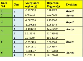
as (0.05, 0.2). These are presented for the model in Table 5.2.

Table 5.2: SPRT analysis for 5 data sets of Time domain data Data

Set N(t)

Acceptance region (≤)

Rejection

Region (≥) Decision

1 ₁ -0.192413 0.409923 Reject

2 1 5.450218 9.227729 Accept

3 1 -1.097859 1.955607 Reject

2 -1.089988 1.963344

4 1 -1.463770 14.417935 Accept

2 9.219935 22.746529

5

1 0.342287 10.149104

Reject

2 -0.352199 8.690369

3 -1.141871 2.044587

6 1 -0.263947 47.757861 Accept

Http://www.ijetmr.com©International Journal of Engineering Technologies and Management Research [25] From the above table it is observed that a decision of either to accept or reject the system is reached well in advance of the last time instant of the data.

6. Conclusion

The table 5.2 of Time domain data as exemplified for 6 Data Sets shows that Rayleighmodel is performing well in arriving at a decision. Out of 6 Data Sets of Time domain the procedure applied on the model has given a decision of acceptance for 3 and Rejection for 3 at various time instant of the data as follows. Data Set #1, #3 and #5 are Rejected at 1st, 2nd and 3rdinstant of time respectively. Data Set #2, #4 and #6 are accepted at 1st_{, 2}nd _{and 2}nd _{instant of time respectively.}

Therefore, by applying SPRT on data sets it can be concluded that we can come to an early conclusion of reliable or unreliable software.

References

[1] Goldberg, D. E.(1989). “Genetic Algorithms in Search, Optimization, and Machine Learning”, Addison-Wesley.

[2] JIANG, H. Y. (2006). "Can the Genetic algorithm be a good tool for software engineering Searching problems?" Proceedings of the 30th IEEE International computer software and applications conference (COMPSAC 2006), PP. 362-366, Chicago, USA.

[3] Krishna Mohan. G and Satya Prasad. R. (2011). “Detection of Reliable Software using SPRT on Time Domain data”, International Journal of Computer Science, Engineering and Applications (IJCSEA) Vol. 1, No. 4, pp[92-99].

[4] Lyu, M.R. (1996). “The hand book of software reliability engineering”, McGrawHill & IEEE Computer Society press.

[5] Pham. H., (2006). “System software reliability”, Springer.

[6] Reckase, M. D. (1983). “A procedure for decision making using tailored testing”, In D. J. Weiss (Ed.), New horizons in testing: Latent trait theory and computerized adaptive testing (pp. 237-254). New York: Academic Press.

[7] Satyaprasad (2007).”Half logistic Software reliability growth model “Ph.D Thesis of ANU, India. [8] Stieber, H.A. (1997). “Statistical Quality Control: How To Detect Unreliable Software Components”, Proceedings the 8th International Symposium on Software Reliability Engineering, 8-12.

[9] Wald. A., (1947). “Sequential Analysis”, John Wiley and Son, Inc, New York.

[10] Xie, M., Goh. T.N., Ranjan.P. (2002). “Some effective control chart procedures for reliability monitoring” -Reliability engineering and System Safety 77 143 -150.

*Corresponding author.