https://doi.org/10.5194/gmd-12-5113-2019 © Author(s) 2019. This work is distributed under the Creative Commons Attribution 4.0 License.
A comparative assessment of the uncertainties of global surface
ocean CO
2
estimates using a machine-learning ensemble
(CSIR-ML6 version 2019a) – have we hit the wall?
Luke Gregor1,2,3, Alice D. Lebehot1,2, Schalk Kok4, and Pedro M. Scheel Monteiro1 1SOCCO, Council for Scientific and Industrial Research, Cape Town, 7700, South Africa 2MaRe, Marine Research Institute, University of Cape Town, Cape Town, 7700, South Africa
3Environmental Physics, Institute of Biogeochemistry and Pollutant Dynamics, ETH Zürich, 8092 Zürich, Switzerland 4Department of Mechanical & Aeronautical Engineering, University of Pretoria, Pretoria, 0028, South Africa
Correspondence:Luke Gregor ([email protected]) Received: 14 February 2019 – Discussion started: 5 April 2019
Revised: 5 November 2019 – Accepted: 8 November 2019 – Published: 10 December 2019
Abstract.Over the last decade, advanced statistical inference and machine learning have been used to fill the gaps in sparse surface ocean CO2measurements (Rödenbeck et al., 2015).
The estimates from these methods have been used to con-strain seasonal, interannual and decadal variability in sea–air CO2 fluxes and the drivers of these changes (Landschützer
et al., 2015, 2016; Gregor et al., 2018). However, it is also becoming clear that these methods are converging towards a common bias and root mean square error (RMSE) bound-ary: “the wall”, which suggests thatpCO2estimates are now
limited by both data gaps and scale-sensitive observations. Here, we analyse this problem by introducing a new gap-filling method, an ensemble average of six machine-learning models (CSIR-ML6 version 2019a, Council for Scientific and Industrial Research – Machine Learning ensemble with Six members), where each model is constructed with a two-step clustering-regression approach. The ensemble average is then statistically compared to well-established methods. The ensemble average, CSIR-ML6, has an RMSE of 17.16 µatm and bias of 0.89 µatm when compared to a test dataset kept separate from training procedures. However, when validat-ing our estimates with independent datasets, we find that our method improves only incrementally on other gap-filling methods. We investigate the differences between the methods to understand the extent of the limitations of gap-filling esti-mates ofpCO2. We show that disagreement between
meth-ods in the South Atlantic, southeastern Pacific and parts of the Southern Ocean is too large to interpret the interannual variability with confidence. We conclude that improvements
in surface oceanpCO2estimates will likely be incremental
with the optimisation of gap-filling methods by (1) the in-clusion of additional clustering and regression variables (e.g. eddy kinetic energy), (2) increasing the sampling resolution and (3) successfully incorporatingpCO2estimates from
al-ternate platforms (e.g. floats, gliders) into existing machine-learning approaches.
1 Introduction
The ocean plays a crucial role in mitigating against climate change by taking up about a third of anthropogenic carbon dioxide (CO2) emissions (Sabine et al., 2004; Khatiwala et
al., 2013; McKinley et al., 2016). While the mean state in the global contemporary marine CO2uptake is a widely used
benchmark (Le Quéré et al., 2018), underlying assumptions and limited confidence regarding the variability and long-term evolution of this sink persist. Sparse observations of surface ocean CO2 during winter and in large inaccessible
years (Monteiro et al., 2015; Bakker et al., 2016; Gray et al., 2018).
The community has turned to models and data-based ap-proaches to improve estimates of CO2uptake by the oceans
for periods and regions with poor or no observational cover-age (Wanninkhof et al., 2013b; Rödenbeck et al., 2015; Verdy and Mazloff, 2017). Ocean biogeochemical models are able to capture the general global trend in increasing oceanic CO2
uptake shown by observations but suffer from significant re-gional and interannual (∼1 Pg C yr−1) differences in their es-timates because these models cannot yet accurately parame-terise the marine carbonate system at computationally feasi-ble resolutions (Wanninkhof et al., 2013b). In recent years, data-based approaches, e.g. statistical interpolations and re-gression methods, have become a popular alternative to bio-geochemical models (Lefèvre et al., 2005; Telszewski et al., 2009; Landschützer et al., 2014; Rödenbeck et al., 2014; Jones et al., 2015; Iida et al., 2015). The regression methods try to maximise the utility of existing ship-based observa-tions by extrapolating CO2using proxy variables (observable
from space or interpolated). Extrapolating with proxy vari-ables is possible due to the non-linear relationship between the partial pressure of CO2 (pCO2) in the surface ocean
and proxies that may drive changes in surface oceanpCO2.
Improved access to quality-controlled ship-based measure-ments of surface ocean CO2through the Surface Ocean CO2
Atlas (SOCAT) database, and satellite and reanalysis prod-ucts as proxy variables have aided the development of the data-based methods (Rödenbeck et al., 2015; Bakker et al., 2016).
1.1 The current state of machine learning in ocean CO2estimates
With the increase in the number of statistical estimates of surface ocean CO2, the Surface Ocean CO2 Mapping
(SO-COM) community collated 14 of these methods in an in-tercomparison of “gap-filling” methods (Rödenbeck et al., 2015). The intercomparison gives an overview of the SO-COM landscape, with regression and statistical interpolation approaches making up eight and four of the 14 methods, re-spectively (Rödenbeck et al., 2015). Two model-based ap-proaches were also compared.
While SOCOM intercomparison did not seek to iden-tify an optimal mapping method, it assessed members ac-cording to how well they represented interannual variabil-ity (IAV) relative to climatological surface ocean pCO2
increasing at the rate of atmospheric CO2 concentrations
(Riav). Two methods, the Jena-MLS (mixed-layer scheme) and MPI-SOMFFN (self-organising map feed-forward neu-ral network), achieved lowerRiavscores compared to other members of the comparison. MPI-SOMFFN is a global im-plementation of a two-step clustering-regression approach and has been widely adopted in the literature (Landschützer et al., 2015, 2016, 2018; Ritter et al., 2017). The elegance of
the clustering-regression approach, particularly the cluster-ing step, is that it reduces the problem into smaller parts with more coherent variability and reduces the computational size of the problem per cluster – a beneficial attribute when using regression methods that do not scale well to big datasets.
The SOCOM intercomparison found that the gap-filling methods were in agreement in regions with a large number of seasonally resolving persistent measurements, but the differ-ent methods did not agree in regions where data were sparse (e.g. the Southern Ocean). Similarly, Ritter et al. (2017) found little agreement in the Southern Ocean on seasonal timescales, yet on decadal timescales, there was agreement on the direction of trends between gap-filling methods. 1.2 Measuring the uncertainty of estimates?
The assessment of gap-filling methods is largely limited by the distribution of the observational coverage, which is particularly true for the Southern Hemisphere where data are sparse (Rödenbeck et al., 2015; Bakker et al., 2016). The standard use of root mean squared error (RMSE) and bias as measures of uncertainty gives larger weighting to observation-heavy regions or periods compared with data-sparse regions and periods, potentially leading to underes-timates of uncertainty (Lebehot et al., 2019). Note that the term “error” refers here to the error introduced by the gap-filling method relative to the observations. TheRiav score improves on the standard implementation of RMSE and bias by weighting the uncertainties annually, thus giving a less temporally biased estimate of uncertainty.
Previous studies have compared their methods’ estimates to independent datasets, where measurements ofpCO2 are
not included in the SOCAT datasets (Landschützer et al., 2013, 2014; Jones et al., 2015; Denvil-Sommer et al., 2019). These data serve as good validation data, particularly with the inclusion of derivations ofpCO2from autonomous
plat-forms in the Southern Ocean, a historically undersampled area especially during winter (Boutin and Merlivat, 2013; Gray et al., 2018).
One of the concluding statements in the SOCOM inter-comparison is that pseudo or synthetic data (deterministic model output) experiments should be used to test and com-pare methods. Gregor et al. (2017) did just this, but their study was limited to the Southern Ocean, and the synthetic data did not fully capture the variability represented by ob-servations, in part due to coarse synthetic data resolution (5 d mean and 1/2◦spatially). The authors found that the
ensem-ble average performed slightly better than ensemensem-ble mem-bers, in agreement with ensemble averaging approaches pre-viously used in ocean CO2studies (Khatiwala et al., 2013).
1.3 Aims
The main aim of this study is to present and evaluate a new machine-learning approach to estimate surface oceanpCO2.
We propose the use of an ensemble average, where we hy-pothesise that the “whole is greater than the sum of its parts” as the strengths of the ensemble members are often comple-mentary in such a way to overcome the weaknesses (Khati-wala et al., 2013; Gregor et al., 2017). Further, we aim to evaluate the method for a selection of existing gap-filling methods. From this comparison, we aim not only to gain a sense of our method’s performance but also the state of gap-filling based estimates; i.e. where would we be able to im-prove in future work?
2 Methods
There are two main components to this study: surfacepCO2
mapping with multiple methods and robust error estima-tion from SOCAT v5 gridded product and independent data sources. This study takes a similar two-step approach used in the Japanese Meteorological Agency – multi-linear regres-sion (JMA-MLR) and MPI-SOMFFN approaches, where data are grouped or clustered first, and then a regression al-gorithm is applied separately to each group or cluster. We use the ocean CO2biomes by Fay and McKinley (2014) as
an option for grouping. Alongside this grouping, we use an optimal K-means clustering configuration. Next, four non-linear regression methods are applied to each of the group-ings. The regression methods are support vector regression (SVR), feed-forward neural network (FFN), extremely ran-domised trees (ERT) and gradient-boosting machine (GBM). The latter two approaches are new to the application. These methods are then compared to independent data sources. This is outlined in more detail in the experimental overview be-low.
2.1 Experimental overview
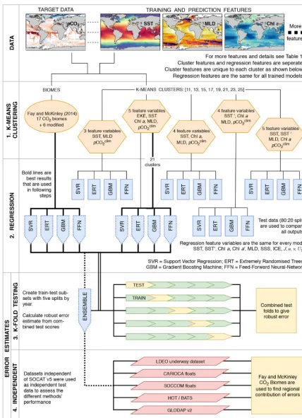
The experimental design, outlined below, is summarised in Fig. 1:
1. In the first step (denoted as “K-means clustering” in Fig. 1), we generate climatological biomes using the oceanic CO2biomes by Fay and McKinley (2014), and
a selection of features variables (five combinations) and number of clusters (a range of 11 to 25 clusters, step-ping by two) resulting in a total of 41 clustering config-urations.
2. Four regression algorithms are applied to each cluster-ing configuration, resultcluster-ing in 164 models (described by the “regression” section in Fig. 1). The test data (isolated from the model training procedure) are used to identify the best-performing clustering configuration with annually weighted bias, RMSE andRiav. The four
regression models for CO2biomes and the four models
from the best-performing clustering configuration (as indicated by the bold lines in Fig. 1) are used in the steps that follow. The selected eight models are aver-aged to create an ensemble average that is included with the eight members for further evaluation.
3. The third step (as represented by the “K-fold testing” section in Fig. 1 and Sect. 2.5) provides a robust un-certainty evaluation based on the training data (SOCAT v5). An iterative test-train approach is applied to esti-mate the bias, RMSE andRiavfor the complete SOCAT v5 dataset (rather than just one test split).
4. The fourth step compares the ensemble average esti-mates of surface oceanpCO2with independent test data
(that are not in SOCATv5, as represented by the “inde-pendent” section in Fig. 1), which allows testing the pre-dictive ability of the ensemble method (Sect. 2.6). Four methods from the SOCOM gap-filling intercomparison study are included for reference.
5. Lastly, all gap-filling methods are compared to identify regions where there is a divergence in the trend and sea-sonal cycle.
2.2 Data: clustering, training and prediction
Standard machine-learning implementation requires a train-ing and a predictive dataset. The traintrain-ing dataset consists of a target variable that is being predicted (in this case,pCO2)
and one or more feature variables that have samples that cor-respond with target samples, e.g. sea surface temperature (SST), Chl a and mixed-layer depth (MLD) co-located in space and time, where feature variables may directly or in-directly influence the target variable. Features variables are used to predict once a machine-learning model has been trained and must thus be available for the full prediction do-main.
Here, we use surface oceanpCO2calculated from the
SO-CAT v5 monthly griddedfCO2 (fugacity of CO2) product
(hereinafter SOCAT v5, as shown in Fig. 2) as the target vari-able (Sabine et al., 2013; Bakker et al., 2016). SOCAT v5 is a quality-controlled dataset that contains observations of sur-face oceanfCO2, which is converted topCO2with
pCO2=fCO2·exp
Patmsurf·B+2·δ R·T
−1
, (1)
Figure 2.Map showing the distribution of the SOCAT v5 monthly gridded product (1982–2016) as a monthly climatology to show how well the seasonal cycle is represented (regardless of the year). The red shading shows grid points where the majority of data occur from May to October, and the blue shading shows grid points where the majority of data occur from November to April.
An important consideration in the use of the SOCAT database is that in situ measurements (i.e. ship measure-ments) are not collected at the surface. The in situ temper-atures that coincide with pCO2in the SOCAT database are
thus different from surface temperature products used to es-timate pCO2 and calculate fluxes (Goddijn-Murphy et al.,
2015; Bakker et al., 2016). The discrepancy in in situ and remotely sensed temperature results in a theoretical differ-ence between pCO2 measured at the ship intake depth and
the surface due to warming or cooling (Takahashi et al., 1993). Goddijn-Murphy et al. (2015) suggest that a correc-tion for the theoretical difference inpCO2 should be made
using the empirical relationship betweenpCO2and
temper-ature (Takahashi et al., 1993). While this merits further co-ordinated consideration by the marine CO2observation
com-munity, we do not apply such a temperature correction in this study, as we aim to be consistent with the earlierpCO2
esti-mates from the SOCOM intercomparison (Rödenbeck et al., 2015). However, we do present the potential impact of this discrepancy in Sect. S2.4.
Feature variables in both the training and predictive datasets are globally gridded products, including satellite ob-servations, in situ measurements and reanalysis products (Ta-ble 1; see Sect. S1 for details). All feature varia(Ta-bles are grid-ded to a monthly frequency onto a global 1◦×1◦
resolu-tion grid. Thereafter, data processing steps are applied as shown in Table 1 and described in detail in the Supplement (Sect. S1), with the final output being a complete dataset ranging from 1982 to 2016. Note that the clustering and re-gression steps use different subsets of the feature variables, as indicated in Table 1.
In this paragraph, we briefly describe the data processing steps shown in Table 1; detailed product descriptions and in-depth processing steps are in Sect. S1. We derive an ad-ditional SST feature, SST0, by subtracting the annual mean of SST from each respective year, leaving the annual mean anomalies (Reynolds et al., 2007; Banzon et al., 2016). We use the log10 transformation of the Globcolour Chla global
product (Maritorena et al., 2010). Cloud gaps and the period before the start of the product (1982–1997) are filled with the climatology (1998–2016), and high-latitude winter regions (where there is no climatology for Chla) are filled with low-concentration random noise to be consistent with regions of low-concentration Chla(Gregor et al., 2017). We derive an additional Chla feature, Chl a0, using the same procedure as described for the SST annual mean anomalies. We use a log10 transformation of MLD from Argo float density
pro-files (Holte et al., 2017) to create a monthly climatology, thus imposing the assumption that there is no interannual variabil-ity. Wind speed is calculated from 6-hourly data using the equation in Table 1 before taking the monthly average. At-mosphericpCO2is calculated withpCO2=xCOatm2 ×Patm,
wherexCOatm2 is the mole fraction of atmospheric CO2(from
ObsPack v3 by Masarie et al., 2014) andPatmis the reanal-ysed mean sea-level pressure (from ERA-interim 2; Dee et al., 2011) – further details for the procedure are in Sect. S1. The climatology of eddy kinetic energy (EKEclim) is calcu-lated fromuandv surface current components (integrated for depth<15 m) from the Globcurrent product (Rio et al., 2014), whereu0 is calculated asu−uand similarly withv (Table 1).
2.3 Clustering and biomes
The seasonal and interannual variability of global surface oceanpCO2is complex due to interactions of various driver
variables acting on the surface ocean at different space scales and timescales (Lenton et al., 2012; Landschützer et al., 2015; Gregor et al., 2018). Machine-learning algorithms ap-plied globally struggle to represent the pCO2 accurately
unless spatial coordinates are included as feature variables (Gregor et al., 2017). This is due to the fact thatpCO2may
respond inconsistently to observable feature variables in dif-ferent regions as it is not possible to observe all feature vari-ables that drivepCO2. A common practice to avoid the
in-clusion of coordinates is to separate the ocean into regions where processes that drivepCO2are coherent and then
ap-ply individual regressions to each region – five of the eight regression methods in Rödenbeck et al. (2015) apply this ap-proach. We adopt two such approaches to develop regions of internal coherence with respect to CO2variability, namely
re-gions defined by biogeochemical properties and clusters de-fined by a clustering algorithm.
Our first “clustering” approach uses the oceanic CO2
Table 1.Summary of the products, variables and data processing steps used for feature variables. The “usage” column indicates the features that are used for the clustering step (identified by C) and for the regression step (identified by R). Abbreviations are used in Fig. 1 and throughout the text. Basic data processing is described in the text with details in the Supplement (Sect. S1).
Group: product Variable Abbreviation Usage Processing Reference
NOAA: dOISSTv2 Sea surface temperature SST C, R – Reynolds et al. (2007);
(AVHRR only) SST seasonal anomaly SST0 C, R SST – annual average Banzon et al. (2016)
Sea ice fraction ICE R –
Met Office: EN4 Salinity SSS R – Good et al. (2013)
CDIAC: ObsPack v3 AtmosphericpCO2 pCO2atm R xCOatm2 ×sea-level pressure Masarie et al. (2014)
UCSD: Argo mixed layers Mixed-layer depth MLD C, R log10(climatology) Holte et al. (2017)
ESA: Globcolour Chla Chla C, R log10climatology filledcloud gaps1982–1997 Maritorena et
Chlaseasonal anomaly Chla0 R Chla– annual average al. (2010)
ECMWF: ERA-Interim 2 uwind u R – Dee et al. (2011)
vwind v R –
Wind speed U10 R
p u2+v2
ESA: Globcurrent Eddy kinetic energy EKEclim C log10
1/2·u02+v02 Rio et al. (2014)
– Day of the year J R sin365j , cos365j –
LDEO:pCO2climatology Surface oceanpCO2 pCOclim2 C Data smoothing Takahashi et al. (2009)
Figure 3. Regions or biomes as defined by Fay and McKinley (2014). Unclassified regions from the original data have been assigned manually in this study and are shown by the separate colours. This modified configuration of the CO2biomes is referred to as BIO23 in this
biomes by establishing thresholds for SST, Chl a, sea-ice extent and maximum MLD. Unclassified regions from the original biomes are manually assigned based on their geo-graphical extent, resulting in six additional regions (Fig. 3). We maintain these as separate regions from the original Fay and McKinley (2014) biomes. Their study originally did not classify these regions in the core biomes because the physi-cal and biogeochemiphysi-cal properties were not accounted for by the set thresholds from their study. This would suggest that drivers of CO2in these regions could be quite different from
the adjacent open-ocean biomes. Note that we may refer to the modified Fay and McKinley (2014) ocean CO2biomes as
“CO2biomes” or as “BIO23” from here on (Fig. 3). For later
analyses, we group certain biomes together, as shown by the brackets above the colour bar in Fig. 3.
We also useK-means clustering, which groups data based on Euclidean distances. More specifically, we implement mini-batch K means from Python’s Scikit-learn package (Sculley, 2010; Pedregosa et al., 2011), which is described in the Supplement (Sect. S2.2; Fig. S2). We apply clustering with various feature combinations and the number of clusters (shown by orange hexagons in Fig. 1). We tested a range of 11 to 25 clusters (stepping by two). The performance of each clustering configuration is not tested with a clustering met-ric; instead, we test the performance based on the test scores of the regressions in the next step as a more complete indi-cator of performance. We find optimal results with respect to RMSE and biases with 21 and 23 clusters. We selected 21 clusters (Fig. S2). Each method of defining regional coher-ence with respect topCO2variability has its methodological
weaknesses so in this study, we adopted the approach of in-corporating bothK means and CO2biomes into the
ensem-ble average (Fig. 1). Although this likely weakens the geo-physical meaning of the ensemble domains, we show that it strengthens the overall performance of the ensemble average. 2.4 Regression
Here, we describe the underlying machine-learning princi-ples of regression. The co-located data (i.e. SOCAT v5) are split into training and test subsets with a roughly 80 : 20 split. The test subset is isolated from the training process to at-tain a reliable estimate of uncerat-tainty. We make the split be-tween training and test subsets based on a random subset of years in the time series (1982–2016): 1984, 1990, 1995, 2000, 2005, 2010 and 2014. We avoid using a shuffled train-test split (completely random), as this leads to artificially low uncertainties in machine-learning algorithms that are prone to overfitting (see the experiment in Sect. S2.1), where the models can reproduce the shuffled test data better, as these data are adjacent to samples of the same ship track.
We further reduce the possibility of overfitting by tuning the hyperparameters for each model to be more generalised, i.e. able to fit the data that the model has not been exposed to. The search for the optimal hyperparameters is achieved with
grid-search cross validation, where a portion of the training subset is iteratively kept separate from the training process for a certain set of hyperparameters (Hastie et al., 2009). The hyperparameters that result in the best score from the grid search are used for the fit with the full training subset (see Sect. S2.3 for more details). We use a variation ofK-fold cross validation called “groupK fold” in Scikit-learn (Pe-dregosa et al., 2011). Rather than having arbitrary splits for each fold, a given grouping variable is used to split the data – in this case, years. Using years as the grouping variable re-duces bias towards the second half of the time series where data are less sparse.
The train-test split and cross validation are applied iden-tically to each of the four machine-learning algorithms for each clustering configuration. We use the following machine-learning algorithms: ERT – Geurts et al. (2006); GBM – Friedman (2001); SVR – Drucker et al. (1997); and FFNs. The details of these methods and how they were tuned are explained in the Supplement (Sect. S2.3). The first two meth-ods, ERT and GBM, are new to this application. SVR has been implemented as a single global domain by Zeng et al. (2017), and FFN is used by several different methods, some of which are in the SOCOM intercomparison (Land-schützer et al., 2014; Zeng et al., 2014; Sasse et al., 2013).
Regression performance is tested using RMSE primarily but also bias (Eqs. 3 and 4 below) andRiav(Eq. 5), with only the models from the best averaged clustering configuration used for the rest of the study.
2.5 Robust biases and root mean square errors
Standard practice in machine learning is to set aside a test subset of the data, as described in Sect. 2.4. We use this standard approach in the second step of our experiment (re-gression comparison) as an estimate of the performance for each of the machine-learning models (164 in total). How-ever, this grouped train-test split gives a bias and RMSE es-timate limited to the random test years of test subset (see Sect. 2.4). To overcome this limitation, we iteratively apply the train-test split method with multiple selections of years. The splits in the test fold are based on a subset of years spaced 5 years apart. We then refactor the five test-fold es-timates into a complete test estimate (with the same structure as the original SOCAT v5), thus giving a complete estimate of bias and RMSE (Fig. 1, step 3). This robust test-estimate method ensures that correct biases and RMSE scores are re-ported even if methods are prone to overfitting (see Sect. S2.1 and Fig. S1). We limit this procedure to only the CO2biome
and best clustered regressions as it has 5 times the computa-tional cost of a single train-test split.
2.6 Method validation data
in-Table 2.Details for the validation datasets. The measured variables are shown (DIC is dissolved inorganic carbon; TA is total alkalinity) along with the estimated accuracy ofpCO2. This includes the propagated uncertainty in the conversion from DIC and TA topCO2as defined
by Lueker et al. (2000), where the estimates marked with∗are an extrapolation of the estimates, as the DIC and TA uncertainties do not match or exceed those listed in the publication. Note that the error estimates for GLODAP v2 are larger than those shown in the table, as measurement uncertainty is defined as±10 µmol kg−1in Bockmon and Dickson (2015). Grid points show the number of data at the same resolution as the feature variables.
Platform Project Measured variable Accuracy (µatm) Reference Grid points
Ship LDEO pCO2equilibrator ±2.5 µatm Takahashi et al. (2017) 16 161
GLODAP v2 DIC+TA >12 µatm at 400 µatm∗ Olsen et al. (2016); 5976 Bockmon and Dickson (2015)
Surface floats CARIOCA pCO2colourimetry ±3.0 µatm Boutin and Merlivat (2013) 613
Profiling floats SOCCOM pH+TA (LIAR) ∼11 µatm at 400 µatm Carter et al. (2016) 1037
Mooring BATS DIC+TA ∼4 µatm at 400 µatm Bates (2007) 246 HOT DIC+TA <7.6 µatm at 400 µatm∗ Dore et al. (2009) 214
Figure 4.The distribution of the validation data. Details of these datasets are given in Table 2. The Hawaii ocean time series (HOT) and the Bermuda Atlantic time series (BATS) are marked as dia-monds to distinguish them as time series stations.
cluded in the Lamont–Doherty Earth Observatory (LDEO) database but not in SOCAT; (2) not measured with an in-frared analyser; or (3) derived from two other variables in the marine carbonate system, where these include dissolved inor-ganic carbon (DIC), pH and total alkalinity (TA) – where the Southern Ocean Carbon and Climate Observation and Mod-eling (SOCCOM) floats use empirically calculated TA.
The uncertainty ofpCO2that is calculated from DIC and
TA is dependent on the accuracy of these two measurements, as well as the derivation ofpCO2with dissociation constants,
for which we use the CBSys package in Python (Hain et al., 2015).CBSysimplements the constants from Lueker et al. (2000) that reports an uncertainty of 1.9 % standard de-viation of the calculated pCO2 where DIC and TA
uncer-tainties are 2.0 and 4.0 µmol kg−1, respectively. The mea-surements in GLODAP v2 are slightly larger than this at 4 and 6 µmol kg−1, which would result in an error larger than 1.9 % – this is 12 µatm for a 400 µatm estimate at a hy-pothetical 3 % error. However, this error may be larger, as
reported in Table 2, where Bockmon and Dickson (2015) showed that the uncertainty for DIC and TA is likely closer to±10 µmol kg−1. While this potentially large error range
may seem concerning, we argue that the inclusion of these data in data-sparse regions is more valuable than their omis-sion. Additionally, GLODAP v2 data have been adjusted on a per-profile basis to minimise the biases through the compar-ison of deep slow-changing ocean properties (Olsen et al., 2016). Williams et al. (2017) estimated the error forpCO2
calculated empirically to be 2.7 %, where TA was calculated empirically with the locally interpolated alkalinity regression (LIAR) algorithm (Carter et al., 2016). Note that the datasets in Table 2 likely suffer from biases unaccounted for due to temperature mismatches as discussed in Sect. 2.2 (Goddijn-Murphy et al., 2015). It is important to note that each of the validation datasets are compared independently of each other, thus avoiding the complications of accounting for the biases between datasets. AllpCO2data are then gridded to
the same time and space resolution as the feature variables (monthly×1◦) usingxarrayandpandaspackages in Python (McKinney, 2010; Hoyer and Hamman, 2017).
2.7 Sea–air CO2flux calculation
Bulk sea–air CO2flux (FCO2) is calculated with FCO2=kw·K0· pCOsea2 −pCO
atm 2
, (2)
whereK0is the solubility of CO2in seawater (Weiss, 1974)
and kw is the gas-transfer velocity calculated from wind
speed using formulation by Nightingale et al. (2000), as this parameterisation was the closest match to in situ observations of CO2 fluxes (Goddijn-Murphy et al., 2016). The
ERA-interim v2 wind product is used to calculatekw.pCOsea2 is
from the gap-filling methods, and pCOatm2 is atmospheric pCO2. All ancillary variables required in these calculations
Rödenbeck et al. (2014). One of the problems with the bulk estimates of sea–air CO2 fluxes is that models of gas
ex-change in the surface layer of the water column are simpli-fied, but there are approaches, such as the rapid equilibrium model, that account for more complex temperature gradients in the upper layer of the surface ocean (Wanninkhof et al., 2009; Woolf et al., 2016). However, for the sake of consis-tency with past studies, we use the bulk approximation of sea–air fluxes (Eq. 2), wherekwis scaled to 16 cm h−1as in
the SOCOM intercomparison (Rödenbeck et al., 2015). 2.8 Relative interannual variability and interquartile
range metrics
2.8.1 Regression metrics
We use bias and RMSE as first-order metrics of model per-formance.
Bias is the mean difference between the target variable and the estimates thereof:
Bias=Xn
i=1
ˆ yi−y
n , (3)
wherenis the number of training samples,yis the array of target data, and yˆ is the corresponding array of estimates. Similarly, RMSE is a measure of the difference between the target variable and the estimates thereof:
RMSE= v u u t n X
i=1
yi− ˆyi2
n . (4)
In our study, these metrics are calculated for each year and then the mean of the annual bias or RMSE scores is taken as a more robust measure of performance in the context of temporally imbalanced data. This is typically done for the global domain unless otherwise stated.
The relative interannual variability metric (Riav) was used in the SOCOM intercomparison by Rödenbeck et al. (2015) to measure how well a method represents the interannual variability of the SOCAT data. The metric furthers the idea of RMSE calculated by year (and region if stated; otherwise global) by normalising annually weighted RMSE to a bench-mark with interannual variability driven only by atmospheric pCO2:
Riav= σ1982–2015(M
iav(t ))
σ1982–2015
Mbenchiav(t )
(5a)
Miav(t )= s
Pn
i=1 yi− ˆyi
n−1 (5b)
Mbenchiav(t )= s
6in=0 yi− ˆyib
n−1 . (5c)
Here, σ is the standard deviation of Miav andMbenchiav , re-spectively, which are both represented as yearly time series.
Equation (5b) and (5c) show the formulation forMiav(t )and Mbenchiav(t ), which represent these metrics for a single year (t). The symbolirepresents individual data points in a particular yeart,y is the observation-based data for that year,yˆ is the predicted data, andnis the number of points in the year and region. The benchmarkedMbenchiav is calculated to normalise Miav.yˆbrepresents the data where IAV has been removed by summing the climatology of the mapped surface oceanpCO2
and the annual trend of atmosphericpCO2. 2.8.2 Ensemble metrics
We use the interquartile range (IQR) between different gap-filling methods as a robust metric of disagreement, in con-trast to the standard deviation, which is sensitive to outliers. IQR is calculated as the third quartile (75th percentile) minus the first quartile (25th percentile). The disagreement between methods is calculated with annually averaged data, with the resulting difference averaged over the time series to arrive at the interannual disagreement (IQRIA). This is calculated per pixel if the representation of the data is spatial (maps) and per time step of a time series.
3 Results
3.1 Regression results
The results from the regression comparisons (step 2 in Fig. 1) are depicted in Fig. 5a–c, which plot the matrix of the (a) av-erage bias, (b) RMSE and (c)Riavfor each combination of the experimental number of clusters and clustering features.
Results show that the configuration that includes EKEclim (column E in Fig. 5a–c) as a clustering feature has the low-est average RMSE and absolute bias for nearly all clustering configurations, regardless of the number of clusters (rows in Fig. 5a, b). The increased dynamics associated with high-EKE regions might change the way pCO2 behaves
fea-Figure 5.Heat maps showing the average cluster(a)bias,(b)RMSE and(c)relative interannual variability (Riav) for different cluster configurations, where smaller scores are better for all metrics. The rows show the number of clusters, and the columns show clustering feature-variable configurations. Each cluster contains the average of the scores for four regression methods: support vector regression, extremely randomised trees, gradient-boosting machine and feed-forward neural network. The black box indicates clustering configurations that perform well across all metrics; note that a value ofRiav<0.3 falls within the best category of performance in Rödenbeck et al. (2015).
tures: SST, log10(MLDclim),pCOclim2 , log10(Chlaclim) and
log10(EKEclim), and is hereinafter abbreviated as K21E (see
Fig. S2 for the distribution of the climatology for these clus-ters).
Comparatively, the Fay and McKinley (2014) CO2biomes
have an average RMSE score of 18.98 µatm (Table 3) but have a lower meanRiav(0.26) and smaller bias (0.03 µatm) than the K21E configuration. Given that the CO2biomes
per-form well and provide an alternate clustering approach, we include the regression estimates. The eight machine-learning models from K21E and BIO23 (four each) were used to create an ensemble average by averaging pCO2 estimates
(CSIR-ML8, Council for Scientific and Industrial Research – Machine Learning ensemble with Eight members).
All regression methods have lower RMSE scores for K21E than for BIO23, but Riav and bias do not indicate that ei-ther of the two clustering approaches is preferable (Table 3). Comparing the RMSE scores of the individual regression methods, we see that the model scores are ranked the same in each cluster from first to last: SVR, ERT, GBM and FFN. However, it is important to note that this ranking does not apply to bias or Riav, where ERT has low RMSE but the largest bias andRiavin each clustering approach. CSIR-ML8 only slightly betters its members, with RMSE and bias scores of 17.25 and 0.04 µatm, respectively. However, the ensemble averageRiav(0.25) is only just less than the average of the ensemble members’ average (0.26).
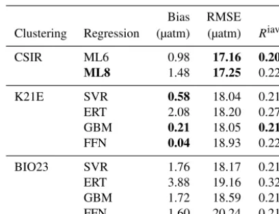
Table 3.Regression scores for the CO2biomes (BIO23), the
clus-tering configuration from column E in Fig. 5 (K21E) and the en-semble average (CSIR-ML8). Abbreviations are as follows: RMSE is the root mean square error;Riavis the relative interannual vari-ability (Eq. 5). Regression methods are as follows: SVR is sup-port vector regression; ERT is extremely randomised trees; GBM is the gradient-boosting machine; FFN is the feed-forward neural network. Bold values are significantly lower than the mean for that column (p <0.05 for the two-tailedZtest; absolute values are used for the bias column).
Bias RMSE Clustering Regression (µatm) (µatm) Riav
CSIR-ML8 0.04 17.25 0.25
K21E SVR −0.45 17.95 0.24
ERT 0.84 17.96 0.36
GBM −0.32 18.21 0.24 FFN −0.30 18.82 0.27
BIO23 SVR −0.19 18.47 0.15
Figure 6.Annually averaged(a)bias and(b)RMSE for the eight individual regression methods in Table 3: BIO23 (dashed lines) and K21E (solid lines). The dotted black lines show the ensemble averages for all eight models (CSIR-ML8), and the solid black line shows metrics for the ensemble average of the SVR, GBM and FFN (CSIR-ML6) from BIO23 and K21E. The grey-filled area in panel(b)shows the number of observations per year, and black triangles show the years that are isolated as the test subset. The vertical dashed grey line demarks 1990, prior to which there is a large positive bias.
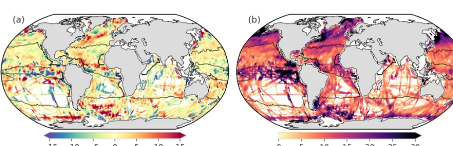
Figure 7.Panel(a)shows the biases from the robust test estimates; panel(b) shows the RMSEs for CSIR-ML6. Convolution has been applied to panels(a)and(b)to make it easier to see the regional nature of the biases and RMSE. Figure S8 shows the bias for every ensemble member. Black lines show the regions as defined in Fig. 3.
3.2 Robust RMSE, bias andRiav
Here, we study the change in the bias and RMSE for all se-lected methods (i.e. K21E, BIO23 and CSIR-ML8; Table 3) across 1982–2016 (Fig. 6). Most notable is that bias scores for all models have the same interannual tendencies, with a positive bias at the beginning of the time series (1982 to
Table 4.The robust estimates of bias, RMSE andRiavfrom 1982 to 2016 for BIO23, K21E and the ensemble averages, CSIR-ML6 and CSIR-ML8, where the first excludes the ERT method. Bold values are significantly lower than the mean for that column (p <0.05 for the two-tailedZtest; absolute values are used for the bias column). See Table S1 for further comparisons between different ensemble average configurations.
Bias RMSE Clustering Regression (µatm) (µatm) Riav
CSIR ML6 0.98 17.16 0.20
ML8 1.48 17.25 0.22
K21E SVR 0.58 18.04 0.21 ERT 2.08 18.20 0.27 GBM 0.21 18.05 0.21
FFN 0.04 18.93 0.22
BIO23 SVR 1.76 18.17 0.21 ERT 3.88 19.16 0.32 GBM 1.72 18.59 0.21 FFN 1.60 20.24 0.21
but this is likely since selected test years (black triangles in Fig. 6b) fall on years of low bias. While FFN has the largest RMSE (18.93 and 20.24 µatm for K21E and BIO23), it has a smaller bias compared to other regression methods (0.04 and 1.60 µatm, respectively), motivating including FFN re-gressions in the ensemble average (Table 4). Conversely, the ERT approach has a significant positive bias likely due to the method’s resilience to outliers, where sparse measurements could be treated as outliers (2.08 and 3.88 µatm for K21E and BIO23, respectively, withp >0.95 for both values; Ta-ble 4; Gregor et al., 2017). A second ensemTa-ble average with-out ERT regressions, thus with six members (CSIR-MLR6 version 2019a; hereafter called CSIR-ML6), has lower biases compared to CSIR-ML8 (0.98 and 1.48 µatm, respectively; Table 4).
Similar to the biases, RMSEs for all models (Fig. 6b) have similar interannual tendencies and variability, with a sharp peak in the year 2000 (>20 µatm, where the mean RMSE is 18.61 µatm). The increased RMSE scores are likely due to the spatial distribution of sampling density (see Fig. S7); e.g. an increase in sampling in the high latitudes during spring and summer, a region and period of high variability and bio-geochemical complexity, would increase the weight of these data in the final RMSE calculation, thus resulting in larger RMSE scores. The increase in the number of samples from 2002 to 2016 results in a sharp decrease in RMSE (<19 µatm for the majority of this period). Both ensemble averages per-form slightly better than all other methods for the majority of the time series with RMSE scores of 17.16 and 17.25 µatm for CSIR-ML6 and CSIR-ML8, respectively (see Table S1 comparisons of ensemble averages with different members).
TheRiavscores for the robust errors (Table 4) are lower than train-test results with a single split reported in Table 3, likely due to an increase of standard deviation for the IAV benchmark (Eq. 5). The lowest score is held by CSIR-ML6 (0.20) and is lower (better) than the average for its members (0.21). TheseRiavestimates compare well to the Jena-MLS and SOM-FFN, which both scored<0.3 (Rödenbeck et al., 2015).
The spatial distribution of the bias and RMSE is now stud-ied for CSIR-ML6 (Fig. 7a and b, respectively), particularly focusing on the regional patterns emerging from the data. CSIR-ML6 clearly represents the subtropical regions (NH-ST and SH-(NH-ST) with relatively low biases and RMSE scores (|bias|<5 µatm and RMSE<10 µatm). The equatorial re-gions (EQU), especially the eastern Pacific, contrasts this with large uncertainties in both bias and RMSE (>|10 µatm| and 30 µatm, respectively). The high-latitude oceans (NH-HL and SH-(NH-HL) have considerable uncertainties due to the large interannual variability of surface oceanpCO2caused
by the formation and retreat of sea ice (around Antarctica; Ishii et al., 1998; Bakker et al., 2008) and phytoplankton spring blooms (Atlantic sector of the Southern Ocean, North Pacific and Arctic Atlantic; Thomalla et al., 2011; Lenton et al., 2013; Gregor et al., 2018). There are two bands of overestimates on the southern and northern boundaries of the North Atlantic Gyre, where the latter coincides with the Gulf Stream. Regression approaches may be prone to a positive bias in the North Atlantic, as this was also shown by Land-schützer et al. (2013, 2014).
In summary, the robust test estimates show that there is a positive bias inpCO2predictions before 1990 for all
mod-els, but it is largest for ERT, and excluding these models from the ensemble results in betterpCO2predictions. The
spatial evaluation of the performance metrics for CSIR-ML6 shows that regions with specific oceanic features (e.g. west-ern boundary currents) mostly have positive biases. However, it is important to note that these uncertainty assessments are limited as the characteristics and biases of the dataset are in-trinsic to the models. Validation with independent data is thus a more reliable estimate of the performance of these methods. 3.3 Validation with independent datasets
Here, we validate the accuracy of pCO2 estimates from
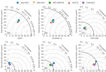
Interpo-Figure 8.Taylor diagrams comparing thepCO2estimates of five gap-filling methods (represented by the different markers) with validation
datasets (Table 2) for the period 1990–2015. Each validation dataset has its own Taylor diagram, as labelled on the bottom axes. The black marker on the bottom axis in each subplot represents the validation dataset and the black arc shows the standard deviation thereof. The closer the gap-filling estimates are to this point, the better the model’s performance, in terms of variance, centred RMSE and correlation (for bias information, see Table 5). The solid grey arcs show the centred RMSE for the datasets (with bias removed). A description of the gap-filling methods from independent studies is provided in the text (Sect. 3.3).
lation (UEA-SI version 1.0; Jones et al., 2015). pCO2
esti-mates by the Jena-MLS were resampled to monthly temporal resolution and interpolated to a 1◦grid using Python’s xar-ray package. Note that these datasets will also suffer from the same temperature biases discussed in Sect. S2.4.
The performance of each gap-filling method is repre-sented with a Taylor diagram for each independent validation dataset (Fig. 8; Taylor, 2001). The most important character-istic learnt from these plots is that the gap-filling methods are tightly bunched for nearly all validation datasets, indicating a similar RMSE, correlation and standard deviation relative to the reference datasets. Poor estimates in Fig. 8a–d may indicate that the training data for gap-filling methods is the limiting factor. Secondly, the gap-filling methods almost al-ways underestimate the standard deviation of the validation datasets, being below the black arched line for all but the sta-tion HOT (Fig. 8e).
All methods fail to represent the standard deviation of the two global validation datasets, LDEO and GLODAP v2 (Fig. 8a, b), with centred RMSE scores greater than 35 µatm. However, calculating RMSE annually results in scores of∼27 µatm for LDEO and∼35 µatm for GLODAP
v2, much lower than shown in Fig. 8a–b, due to high RMSE scores (>40 µatm) for a small subset of years (Sect. S3.4 and Fig. S7). Estimates of the Southern Ocean datasets (Fig. 8c, d), SOCCOM and CARIOCA, have lower RMSE scores (∼16 and∼23 µatm, respectively) relative to LDEO and GLODAP v2. However, for standard deviation scores of similar magnitude and low correlation coefficients, the datasets are not well constrained (Table 5). The SOCCOM dataset also has the largest average absolute bias for esti-mates, with gap-filling methods underestimated by at least 11 µatm (Table 5). This large bias may be because SOCCOM floats have a proportionately large number of winter samples – suggesting that our knowledge of Southern Ocean winter fluxes is largely underestimated (Williams et al., 2017). In contrast, all methods estimate the two time series stations, HOT and BATS (Fig. 8e, f and Table 5), relatively well with correlation scores>0.8 and low average bias∼4.5 µatm.
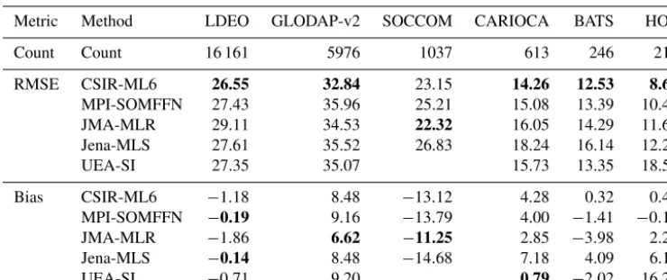
achiev-Table 5.The RMSE and bias for each gap-filling method compared to the validation datasets. For more information on the validation datasets, see Table 2. The first row of data (count) shows the number of gridded samples in the dataset during the period 1990–2015 (that are not in the SOCAT v5 gridded product). Values shown in bold are significantly different from the mean for the column (p <0.05 for the two-tailed
Ztest; absolute values are used for the biases). The UEA-SI method does not have error estimates for SOCCOM floats as these two time series do not overlap.
Metric Method LDEO GLODAP-v2 SOCCOM CARIOCA BATS HOT
Count Count 16 161 5976 1037 613 246 214
RMSE CSIR-ML6 26.55 32.84 23.15 14.26 12.53 8.62
MPI-SOMFFN 27.43 35.96 25.21 15.08 13.39 10.40 JMA-MLR 29.11 34.53 22.32 16.05 14.29 11.64 Jena-MLS 27.61 35.52 26.83 18.24 16.14 12.28 UEA-SI 27.35 35.07 15.73 13.35 18.52
Bias CSIR-ML6 −1.18 8.48 −13.12 4.28 0.32 0.46 MPI-SOMFFN −0.19 9.16 −13.79 4.00 −1.41 −0.12 JMA-MLR −1.86 6.62 −11.25 2.85 −3.98 2.22 Jena-MLS −0.14 8.48 −14.68 7.18 4.09 6.15 UEA-SI −0.71 9.20 0.79 −2.02 16.27
ing low p values. No single method dominates the biases, with JMA-MLR and MPI-SOMFFN each scoring the lowest bias on two occasions. To summarise, all gap-filling methods underperform when validated against independent observa-tional products. Tight bunching of gap-filling method scores per validation dataset shows that training data may limit all methods in the same manner.
3.4 The effect of uncertainties on the sea–air CO2flux interannual variability
In this section, we assess the regional implications of the differences in gap-filling methods’ estimates (within CSIR-ML6 and the four independent methods described in Sect. 3.3) of the sea–air CO2 flux (FCO2) over the period
1990 to 2016. FCO2 was calculated using the same
gas-transfer velocity and solubility for each gap-filling method (Sect. 2.7). Differences in FCO2 are thus driven by
varia-tions inpCO2from each gap-filling method.
The averageFCO2for 1990–2016 by CSIR-ML6 (Fig. 9a)
contextualises the regional distribution of fluxes: strong out-gassing in the equatorial Pacific, strong sink in the midlat-itudes, a moderate uptake for the most part of the subtrop-ics and weak source in the majority of the Southern Ocean (in agreement with, e.g. Takahashi et al., 2009). The global annual time series for FCO2 as simulated by CSIR-ML6
(Fig. 10a) indicates a strengthening for 2000 to 2016 (as for the other methods). To give spatial context to this strengthen-ing, we display the differences inFCO2between 2016 and
2000 (Fig. 9b), since those are the two years where the dif-ference in globalFCO2is greatest for CSIR-ML6 (Fig. 10a).
Note that Fig. 9b serves as a snapshot for the change in FCO2 between those two years, whose interpretation
can-not be linked to an overall anthropogenically forced change
as the comparison between the two years could reflect inter-annual, decadal or multi-decadal variability. The differences inFCO2 between 2016 and 2000 are negative in the high
latitudes and moderately positive in the subtropics, indicat-ing a respective increase and decrease in the CO2ocean
up-take between the two years. The eastern equatorial Pacific is the only region that shows a considerable increase inFCO2
(>10 g C m−2yr−1) between the two specific years. The annual change in FCO2 is also studied for the
different regions. The Southern Hemisphere high-latitude (SH-HL) region is the strongest contributor to the trend (Fig. S10b), where there is a steady increase in the uptake of CO2since the 2000s for all methods (Landschützer et al.,
2015; Gregor et al., 2018). On average, the Northern Hemi-sphere high latitudes (NH-HL) are a weaker sink relative to the SH-HL, because the SH-HL is more than double the area of the NH-HL (Fig. S10c). The equatorial (EQU) region is the only persistent source of CO2 to the atmosphere (also
seen in Fig. 9a). The subtropical regions (Fig. 10c, e) con-tribute to global flux on similar orders of magnitude; how-ever, there is a large divergence between gap-filling methods in the SH-HL.
We use the average interquartile range between the 1-year rolling mean estimates (IQRIA) as a measure of agreement or divergence between gap-filling methods, where large val-ues indicate a divergence (Sect. 2.8.2). We also show the IQRIA scaled to the range of the regional interannual vari-ability (max–min) as a percentage (relative IQRIA), which shows if the trend for a particular region is agreed on by all methods (the smaller the percentage, the better the agree-ment across methods). The disagreeagree-ment between methods in the SH-ST is substantial (Fig. 10e), with divergingFCO2
throughout the period with an IQRIAof 0.11 Pg C yr−1 and
Figure 9. (a)Average sea–air CO2fluxes (FCO2) of CSIR-ML6 for 1990 to 2016, whereFCO2is calculated as shown in Eq. (2). Negative FCO2(blue) indicates regions of atmospheric CO2uptake.(b)The differences betweenFCO2in 2016 and 2000, which are the minimum
and maximum of global ocean uptake flux (FCO2) estimates, respectively (for CSIR-ML6 in Fig. 10a). Black lines show the regions as
defined in Fig. 3.
SH-HL region (Fig. 10f) is 0.08 Pg C yr−1, but the relative IQRIA is lower at 14 %, indicating that all methods agree on the observed strong trend. Compared to the Southern Hemisphere, the Northern Hemisphere regions are both rel-atively well constrained, with IQRIA estimates of 0.04 and 0.05 Pg C yr−1 for the NH-ST and NH-HL regions, respec-tively (Fig. 10c, d). However, a larger relative IQRIAof 20 % suggests that the interannualFCO2estimates in the NH-ST
region are potentially not resolving the trend, or more likely that there is a weak trend with a small difference between the minimum and maximum interannual estimates ofFCO2.
The EQU region (Fig. 10b) has an IQRIAand relative score at 0.03 Pg C yr−1and 14 %.
The CSIR-ML8 method is not included in the IQRIA cal-culations but is included in Fig. 10 to show the impact of the ERT models’ positive bias inpCO2onFCO2(Fig. 6a).
The biases are positive at the beginning and negative end of the time series, with the average absolute difference between the CSIR methods being 0.08 Pg C yr−1. The positive biases have the strongest impact on the SH-ST that occupies 36 % total area (Fig. S10c), with only 11 % of the total observa-tions in SOCAT, suggesting that this method is sensitive to imbalanced datasets.
3.5 Regional disagreement between methods
In order to better understand the regional distribution of the uncertainties inFCO2, we assess the level of agreement
be-tween independent gap-filling methods in their interannual surface oceanpCO2estimates (Fig. 11). We use pCO2for
this representation as no spatial integration occurs – only time averaging.
The interannual estimates of IQRIA (Fig. 11a) show the disagreement between methods is relatively small in the majority of the ocean (<6 µatm), with the exceptions be-ing the Southern Ocean, South Atlantic, southeastern Pacific
and eastern equatorial Pacific with differences of>10 µatm, where these regions coincide with regions of low sam-pling density (Fig. 2). The IQRIA scaled to the maximum– minimum range of interannualpCO2suggests that the
NH-ST trend is relatively well constrained (<10 %), which is in conflict with the IQRIA for FCO2 in Fig. 10c (where the
relative IQRIA is 20 %). The disagreement may stem from the magnifying impact that wind speed has onFCO2; i.e.
small differences in pCO2 may become large when fluxes
are calculated. The same principle may apply to the EQU in Fig. 11b, where relative IQRIAis large (>10 %) forpCO2,
but low wind speeds result in a low relative IQRIAforFCO2
(7 % in Fig. 10b). The largest relative IQRIAscores occur in the SH-ST (>10 % in Fig. 11c) where data are sparse, specif-ically the South Atlantic and southeastern Pacific (Fig. 2a). The relative IQRIAscores suggest that the gap-filling meth-ods agree on pCO2 in the SH-HL east of the Greenwich
meridian (>0◦E).
In summary, we show that there is an agreement between gap-filling methods in the Northern Hemisphere for interan-nualpCO2, but the methods show considerable disagreement
in the Southern Hemisphere, particularly in the subtropics. Disagreements in the equatorial and Southern Hemisphere high-latitude regions are large (>10 %) and should be treated with caution when considering trends in these regions.
4 Discussion
4.1 Not all models are equal
Figure 10.Sea-air CO2 fluxes averaged for regions as shown in Fig. 2:(a)global domain, (b)equatorial regions,(c)Northern
Hemi-sphere subtropical,(d)Northern Hemisphere high latitude,(e)Southern Hemisphere subtropical.(f)Southern Hemisphere high latitude. The coloured lines show the four SOCOM products. The thick and dotted grey lines show the results for CSIR-ML6 and CSIR-ML8, respec-tively. A moving average of 12 months has been applied to smooth the data. Note that they-axis scales differ for the top(a, b). Note that the uncertainties of each model (e.g. bias and RMSE from Fig. 6) are not shown here. The text at the right of each figure shows the number of SOCAT v5 gridded data points for each region (n) and the interannual interquartile range (IQRIA).
an ensemble average of two-step machine-learning models that estimate global surface oceanpCO2. We show robustly
that the CSIR-ML6 method reproduces the available data with greater accuracy than previous methods, albeit in an in-cremental way. Our method is methodologically consistent with regard to feature variables. Though there is variability in the clustering and regression, we create the ensemble average with a good understanding of each model’s biases (Figs. 6 and S8). The argument that ensemble averages reduce trans-parency is also somewhat diminished by the fact that little additional information that can be gained from highly non-linear models, with the exception of basic diagnostics such as feature-variable importance (see Fig. S11) from decision-tree-based approaches (Pedregosa et al., 2011; Castelvecchi, 2016). Our results thus show that there is, in fact, a bene-fit in creating an ensemble average of models (Table 5), and
if carefully implemented, it is an additional tool that can be used to reduce the uncertainties in gap-filling estimates of pCO2.
It could be argued that an exhaustive search for the op-timal configuration (Fig. 5) for CSIR-ML6 may result in poorly trained individual models. However, we think that the merit of introducing and assessing regression algorithms new to the application (for gradient-boosting machines and extremely randomised trees) outweighs the marginal loss in potential performance for individual methods. Moreover, lessons learnt from our study can be used to improve on fu-ture iterations. It also makes the case for ensemble averages stronger, as the CSIR-ML6 performs well relative to other gap-filling methods.
Figure 11. (a)The magnitude of the interannual disagreement between independent gap-filling methods (IQRIA) as shown in Fig. 10; hence, low IQRIAindicates good agreement amongst the different methods.(b)Level of agreement on the interannual variability across methods (in %), more specifically IQRIAscaled by the difference between the maximum and minimum values for interannualpCO2(the range).
as a clustering feature variable leads to an improvement in bias and RMSE for nearly all numbers of clusters, albeit a small improvement. Increased intraseasonal variability of pCO2 appears to be associated with regions of high EKE
compared to low EKE regions (Monteiro et al., 2015; du Plessis et al., 2017, 2019). Moreover, the importance of EKE as a part of the clustering constraints also shows that more thought should be given to how we samplepCO2in
high-EKE regions and at what resolution regression methods are run at.
Our findings suggest the following about the individual re-gression methods: the SVR and GBM algorithms produce good estimates with lower RMSE scores and biases, the FFN approach has larger RMSE scores yet low biases than the other methods, and the ERT approach has low RMSE scores but large biases in the estimates (Fig. 6a, b; Table 4). We do not include the ERT approach in the ensemble average (CSIR-ML6) due to the large time-evolving biases, suggest-ing that ERT (with our tunsuggest-ing) is not suitable for estimatsuggest-ing surface oceanpCO2. The bias in ERT may be due to its
sensi-tivity to imbalanced datasets (Crone and Finlay, 2012), where the data in SOCAT v5 are sparse before 2000. Returning to the above quote by Khatiwala et al. (2013), we thus find that the weaknesses of ERT outweigh its strengths.
4.2 Divergent gap-filling estimates
While we see that the improvements in the performance of gap-filling methods are relatively stagnant (relative to the training and validation data), the differences between the methods’ estimates ofpCO2andFCO2vary significantly in
some regions, particularly in regions where data are sparse, such as in the Southern Hemisphere oceans (Fig. 2). We also find that training the gap-filling methods with limited train-ing data exposes the intrinsic biases of the algorithms, or in the words of Ritter et al. (2017): “the difference [between
Figure 12.The seasonal cycle reproducibility of CSIR-ML6pCO2,
which is a correlation of detrendedpCO2with its own climatology
– the larger the correlation, the stronger the reproducibility of the seasonal cycle (method from Thomalla et al., 2011).
gap-filling methods] is a result of how the spatial and sea-sonal heterogeneity and the sparseness of the data is dealt with”. Conversely, as the number of training data increases, the biases are reduced, and the methods converge.
The Northern Hemisphere subtropical regions are a good example of a region where the gap-filling methods converge (Fig. 11b), as also shown by the low RMSE scores and high correlation for the two mooring stations, HOT and BATS (Fig. 8e, f). One of the reasons that the methods predict the variability well in the subtropics (Fig. 8e, f) is that these re-gions are less biogeochemically complex and driven primar-ily by seasonal changes in SST (Bates, 2001; Dore et al., 2009). This strong SST-driven seasonality in the subtropics is shown by the high seasonal cycle reproducibility (Fig. 12). The gap-filling methods’ divergences also serve as a met-ric to inform where there are not enough data to constrain thepCO2orFCO2estimates; i.e. the divergences inform us
Figure 13.1pCO2trends (p <0.05), where1pCO2is calculated
as the estimated surface oceanpCO2from the CSIR-ML6 method
minus atmosphericpCO2from the CarboScope project (Rödenbeck et al., 2014). The shaded areas show the regions where IQRIA is
>15 %, thus indicating regions where trends should be interpreted with caution.
when scaled to the range of interannual variability (Fig. 11b), should be taken into account when analysing interannual trends of 1pCO2 (Fig. 13). For instance, significant trend
estimates in 1pCO2 for CSIR-ML6 (p <0.05) are
nega-tive for the majority of the global ocean, even in regions where method estimates are too disparate to resolve inter-annual variability (relative IQRIA>15 %; dotted regions in Fig. 13). However, the relative IQRIAis not without its lim-its, as there may be regions where methods are in agreement but share the same biases, thus reporting false confidence in the estimates. Regions of false confidence would most likely occur in data-sparse areas but could only truly be identified with better data coverage in these regions.
4.3 Inching up and over the wall: incremental improvements
In our study, we show that all gap-filling methods suffer from the same uncertainties where there are data to test and val-idate the estimates (Fig. 8), and result in divergences be-tween estimates when there are insufficient data to constrain the methods (Fig. 11b). From these points, it may seem that we may have in fact “hit the wall” in terms of better resolv-ing surface oceanpCO2. In this section, we discuss how we
might overcome this proverbial wall: first, by addressing the existing uncertainty and biases, and then discussing how we could improve on estimates in data-poor regions.
4.3.1 Reducing existing biases
The robust test estimates show that there are regions where training data are not sparse, yet estimates still suffer from large uncertainties (e.g. northern and southern boundaries of the North Atlantic Gyre in Figs. 7a, b and S8). These errors are spatially consistent with those reported by Landschützer et al. (2014). Such regional mismatches between gridded
ob-servations and estimates are likely systematic – meaning that gap-filling methods are not able to resolve the more com-plexpCO2variability at current resolutions (monthly×1◦or
coarser) or with the current regression feature variables (Gre-gor et al., 2017; Denvil-Sommer et al., 2018). It may be pos-sible to reduce these uncertainties with consideration about the drivers of CO2in a specific region. Including appropriate
additional feature variables (if available), such as reanalysis mixed-layer depth products, may improve the uncertainties of gap-filling methods (Gregor et al., 2017). Similarly, in-creasing the temporal and spatial resolution may be able to improve estimates where aliasing occurs in regions of high dynamic variability such as the midlatitude oceans (Monteiro et al., 2015). It is worthwhile to note that increasing the reso-lution may not be the panacea for poor estimates. For exam-ple, the Jena-MLS method is able to estimatepCO2with
rel-ative accuracy (Fig. 8) at a low spatial resolution (≈4◦×5◦;
Rödenbeck et al., 2014); however, with the trade-off in spa-tial resolution, the method is able to increase the temporal resolution to daily estimates.
Another source of bias is the mismatch between the tem-perature at whichpCO2is measured (i.e. at the depth of a
ship’s intake) and the temperature to which pCO2 is
pre-dicted (∼1 m in the case of the dOISSTv2 data; Banzon et al., 2016; Goddijn-Murphy et al., 2015). Goddijn-Murphy et al. (2015) show that this mismatch is considerable in some cases (>5 µatm for large regions, as shown in Fig. S3b). However, the correction of the intake temperature to the re-motely sensed surface temperature also makes the assump-tion that temperature is the only factor that influencespCO2
in the surface layer of the ocean. The correction will thus not account for other processes such as primary production, strat-ification and gas exchange within the surface layer. This is an issue that should be discussed by the community and tested experimentally to assess the impact that these processes may have onpCO2.
4.3.2 Improving estimates in data-poor regions
All gap-filling methods suffer from similar biases and un-certainties (Fig. 8, Table 5) when compared to independent validation data, yet the same methods show vastly differ-ent results in data-sparse regions. These shared uncertainties and regionally consistent divergences between methods are in agreement with past studies, which find that insufficient training data are the limiting factor (Rödenbeck et al., 2015; Landschützer et al., 2016; Ritter et al., 2017; Denvil-Sommer et al., 2018).
we have previously underestimated winter outgassing of CO2
in the Southern Ocean (Gray et al., 2018). Incorporating these new estimates into machine-learning estimates should be a priority for the community as the Southern Ocean plays an important role in anthropogenic CO2 uptake (Gruber et
al., 2019). Incorporating these data successfully into existing models may not be straightforward due to the strong tempo-ral bias of these data toward the end of the time series. For instance, the inclusion of atmosphericpCO2could result in
temporally skewed estimates due to the “memory” effect that including the annually increasing atmospheric pCO2 could
have on estimates.
The complex machine-learning models often used to es-timate pCO2 are prone to overfitting the data, particularly
in regions where data are sparse. Using less complex mod-els, e.g. multi-linear regression, in such regions would re-duce the risk of overfitting the data. A regionally weighted ensemble approach may be an eloquent way to address this problem. In regions with sparse data coverage, simpler mod-els could be favoured, while more complex modmod-els could be weighted more in regions with more data. However, the user would have to apply a potentially subjective model-complexity ranking for each approach. This may work well in the subtropical gyres where pCO2 has a strong
sea-sonal signal driven primarily by temperature (Fig. 12; Taylor, 2001).
One of the weaknesses of our study is that our approach is similar to other regression methods (e.g. MPI-SOMFFN by Landschützer et al., 2014, and JMA-MLR and LSCE-FFNN by Denvil-Sommer et al., 2019) that predict pCO2
based on the instantaneous physical and biological variables without regard for past states. There is thus a need to ex-plore methods that incorporate the past state into future state estimates. This includes assimilative modelling approaches, such as B-SOSE (biogeochemical Southern Ocean state es-timate), which would also provide greater understanding of the driver for changes in surfacepCO2(Verdy and Mazloff,
2017). These methods may be able to provide better con-straints on pCO2 in data-poor regions. However, these
as-similative models are not yet in a stage to fit the data closely (Verdy and Mazloff, 2017).
5 Summary
Our study suggests that we may be reaching the limits of gap-filling methods’ abilities to reduce uncertainties, as shown by the limited incremental improvement in errors by the ensem-ble method we compare with established methods. Signifi-cant uncertainties still prevail across all gap-filling methods, most likely limited by the extent of basin-scale observational gaps in the Southern Hemisphere as well as sampling aliases in mesoscale intensive ocean regions. We propose ways in which the surface ocean CO2 community can improve
es-timates within the bounds of the current observations and make recommendations for future observations.
We introduce a new surface ocean pCO2 gap-filling
method that is a machine-learning ensemble average of six two-step clustering-regression models (CSIR-ML6 ver-sion 2019a). An exhaustive search process was used to find the best K-means clustering configuration which was used alongside the Fay and McKinley (2014) oceanic CO2
biomes. The regression models applied to each clustering method are support vector regression, feed-forward neural networks and gradient-boosting machines. We show that the ensemble average of the six methods marginally outperforms each of its members, thus promoting the idea that averag-ing model estimates, each with different strengths and weak-nesses, result in an improvement in the overall estimates.
The CSIR-ML6 (version 2019a) approach was compared to validation data alongside four other methods from the SO-COM intercomparison study (Rödenbeck et al., 2015). Our new method marginally outperformed the SOCOM methods when comparing RMSE scores for the validation data but fared equally on biases. Despite this improvement, all meth-ods had errors of roughly the same magnitude, suggesting that the methods resolvepCO2 equally outside the bounds
of the training data.
Closer assessment of the spatial distribution of errors shows that there is spatial coherence between regression ap-proaches for the Northern Hemisphere. Some of these errors coincide with regions of high dynamic variability or complex biogeochemistry, suggesting that increasing the spatial and temporal resolution of gap-filling methods could improve es-timates. Moreover, introducing additional feature variables for regression, such as eddy kinetic energy, may improve es-timates in these regions.
A comparison of the distribution of mismatches inpCO2
between gap-filling methods shows that there are regions (primarily in the Southern Hemisphere) where the compared methods, as an ensemble, cannot resolve interannual variabil-ity ofpCO2 and as such, trends analyses in those regions
should be interpreted with caution. These large mismatches likely occur due to amplification of algorithm specific biases in sparse areas. We suggest that an ensemble with data-density-driven weighting for model complexity could be a way to reduce potential overfitting in data-sparse regions. We also urge the community to focus on incorporating new mea-surements from autonomous platforms such as thepCO2
de-rived from pH measured by biogeochemical Argo floats and new platforms such aspCO2-capable Wavegliders.