Complex roots of polynomials and their computation with the help of Scientific Calculators

(1)

Mohd Yusuf Yasin / BIBECHANA 9 (2013) 18-27 : BMHSS, p.18 (Online Publication: Nov., 2012)

BIBECHANA

A Multidisciplinary Journal of Science, Technology and Mathematics ISSN 2091-0762 (online)

Journal homepage: http://nepjol.info/index.php/BIBECHANA

Complex roots of polynomials and their computation with the help

of Scientific Calculators

Mohd Yusuf Yasin

ECE Department, Integral University, Lucknow, UP, India Phone: (office)091-522-2890812, (mobile)091-9335924865,

Email: [email protected]

Article history: Received 10 March, 2012; Accepted 2 August, 2012

Abstract

Real numbers are something which are associated with the practical life. This number system is one dimensional. Situations arise when the real numbers fail to provide a solution. Perhaps the Italian mathematician Gerolamo Cardano is the first known mathematician who pointed out the necessity of imaginary and complex numbers. Complex numbers are now a vital part of sciences and are used in various branches of engineering, technology, electromagnetism, quantum theory, chaos theory etc. A complex number constitutes a real number along with an imaginary number that lies on the quadrature axis and gives an additional dimension to the number system. Therefore any computation based on complex numbers, is usually complex because both the real and imaginary parts of the number are to be simultaneously dealt with. Modern scientific calculators are capable of performing on a wide range of functions on complex numbers in their COMP and CMPLX modes with an equal ease as with the real numbers. In this work, the use of scientific calculators (Casio brand) for efficient determination of complex roots of various types of equations is discussed.

Keywords: Scientific calculators; Calculator techniques; Complex roots; Complex domain computation skills, Numerical techniques

1. Introduction

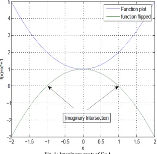
The complex number is a great reality of modern sciences, of which one can never get rid off. There are real examples that can never yield to real solutions.

1 )

(

x

=

x

2

+

f

(1)

(2)

Mohd Yusuf Yasin / BIBECHANA 9 (2013) 18-27: BMHSS, p.19 (Online Publication: Nov., 2012)

A complex number contains a real part accompanied with an imaginary part, and therefore can only be expressed in a two dimensional plane. Real part lies in the usual real plane, but the imaginary part needs be placed in the second direction. The complex numbers can be expressed in any system of representation like rectilinear, polar, spherical etc., but will always need two components to handle. This renders complexity to any computational procedure involving complex numbers.

) ( ) ( ) )(

( ₁ ₁ ₂ ₂ ₁ ₂ ₁ ₂ ₁ ₂ ₁ ₂

2

1z x iy x iy x x y y i x y x y

z = + + = − + + (2)

2 2 2 2 2 1 1 2 2 2 2 2 2 1 2 1 2 2 1 1 2

1 ( ) ( )

) ( ) ( y x y x y x i y x y y x x iy x iy x z z + − + + + = + + = (3) 1 − ≡

i or i2 ≡−1 (4)

Eq.2 and Eq.3 show the additional complexity of computation in case of dealing with complex numbers [2], z being a complex number.

2. Calculator Techniques

Casio brand scientific calculators usually posses a temporary register under the key “Ans”. This register automatically modifies after each computation, and holds the current result. The same key also holds the real and imaginary parts of a result under “CMPLX” mode, which is directly accessible through “Re↔Im” key. While handling complex numbers recursively, this “Ans” key is quite useful same as it is in case of problems handling with real numbers [3]. “Ans” key can be used as variable in both recursive and non recursive procedures.

3. Complex number handling in scientific calculators

In this work, calculators of Casio 991/570 series (991W/115W, 991W/115W, 991MS,

fx-991ES etc.) are under consideration [4,5]. These calculators offer help to tackle with complex number in

different ways. In normal computing mode “COMP”, conversion function POLAR⇔RECTANGULAR

is operational. This function stores the result under memory “E” and “F”. This function is helpful for conversion among rectangular and polar coordinates, since for complex numbers, multiplication and division are easier in polar form whereas addition and subtraction are simpler in rectangular form.

R RECTANGULA

(3)

4. Complex Roots

The fundamental theorem of algebra states a polynomial f(x)=0 of order “n” and with complex coefficients, will have exactly “n” complex roots, complex number is being the more general number [1], a real number is a complex number that contains no imaginary part. From above it is simple to deduce various cases like (a) a polynomial with only real coefficients can have real, complex or imaginary roots, (b) a polynomial with some complex or imaginary coefficients must have one or more complex or imaginary roots, (c) if the polynomial f(x)=0 tends to have imaginary roots, and all of its coefficients are only real, then the complex roots shall appear in complex conjugate pairs. Imaginary number is a complex number with imaginary coefficient, a real number is with only real coefficient, and a complex number is one which contains both real and imaginary coefficients. Complex roots arise due to the nature of functions which do not have any intersection with the real axis.

(4)

Eq.1 does not yield to a real solution. However, it can be solved for imaginary roots, x=±i. These roots can be represented as intersection of the Eq.1 with imaginary axis or the intersection of the flipped plot of Eq.1 with real axis

5. Calculation of complex roots

It is suggested by the fundamental theorem of algebra that both the real and complex roots of a given

polynomial are possible [1]. These roots can be determined by using a root finding method of general

nature. One possible method is Newton – Raphson, which is found quite reasonable in such analyses [2]. This method has a reasonably high convergence rate to estimate a root, and generally yields even to the

less meaningful initial approximations. This method is found suitable for the analyses of the complex

polynomials, functions and for real and complex roots. According to the Newton – Raphson method, the

root of a polynomial f(x)=0 is approached by using Eq.5.

)

(

)

(

' 1

n n n

n

x

f

x

f

x

₊

=

−

(5)

Where

x

_n is a previous estimate of the root,

x

_n₊₁ is the new improved approximation and

f

'

(

x

_n

)

is the first derivative of

f

(

x

_n

)

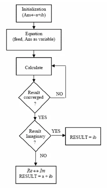
[2].

6. Complex root determination with calculator

The calculator is set to “CMPLX” mode. Initial approximation a+ib is suitably chosen to determine a root and is fed to be in the register under the “Ans” key. Using Eq.5, a similar equation is developed for the problem and is fed to the calculator in terms of the “Ans” as variable. The solution is converged after a few clicks of the “=” key. This scheme is shown by the flow graph of Fig.2.

In the following sections, two examples are considered to demonstrate how easy it is to approach the final accurate result recursively in case of complex root. In both these examples, due to their simplicity and

excellent bidirectional approach to the final accurate solution, the simple Newton – Raphson method is

employed.

7.1 Calculators referred

In this article, scientific calculators referred are casio models like 991W, 991W, 115W,

fx-991MS, fx-991ES etc. or later versions which can work on and display scientific equations [4,5].

7.2 Equations with real coefficients and imaginary roots

Eq.1 or similar equations can be considered here, which contain roots in conjugate pairs. Solving Eq.1 the

(5)

i

x

=

±

(6)

The procedure for determining a root of Eq.1 can be obtained using Eq.5. Thus













−

=

+

n n n

x

1 12

1

(7)

Using a calculator, the Eq.7 can be rewritten as

(

1

)

2

1 − −

= Ans Ans

Ans (8)

Various possibilities on the basis of the initial approximation are as follows.

1.

Ans

←

1 ±

i

(COMPLEX - initial approximation)

Ans ← 0.25+0.75i

Ans ← -0.075+0.975i

Ans ← -1.7157e-3 +0.9973i

Ans ← -4.642e-6 +1.00000216i

(6)

Ans ← 1.002866e-11 + i

Ans ←←←← i

The root smoothly converges to the solution and answer is available after the fifth press of the “=” key.

2.

Ans

←

0 .

5 i

(IMAGINARY - initial approximation)

Ans ← 1.25i

Ans ← 1.025i

Ans ← 1.00030i

Ans ← 1.000000046i

Ans ←←←← i

3.

Ans

←

1 .

0

(REAL - initial approximation)

In this option, the root either oscillates or prematurely terminates.

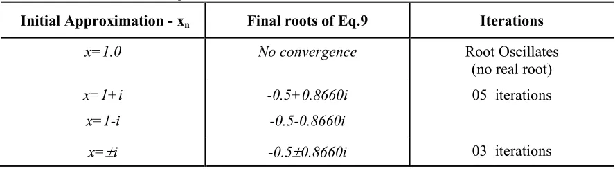
7.3 Equations with real coefficients and complex roots

Let

)

1 (

)

(

x

=

x

2

+

x

+

f

(9)

Both roots of this equation are complex and are

)

866 .

50000

.

0 )(

866 .

0 5000

.

0 (

)

1 (

)

(

x

2

x

i

x

i

f

=

+

=

+

(10)

Using the method described here, the root approximating equation for Eq.9 is written as

(

2

₋

1

)

/(

2 ₊

1 )

=

Ans

(11)

Table 1: Solution details of Eq.9

Initial Approximation - xn Final roots of Eq.9 Iterations

x=1.0 No convergence Root Oscillates (no real root)

x=1+i x=1-i

-0.5+0.8660i -0.5-0.8660i

05 iterations

(7)

7.4 Equations with real coefficients and mixed roots

Let an arbitrary equation, and it’s roots are

) 1 )(

5 . 0 ( )

(x = x− x2 +x+

f (12)

;

866 .

0

5 .

0 ;

5 .

0 x

i

x

=

−

±

(13)

Applying the above algorithm, the convergence detail to the roots are as follows.

Table 2: Solution details of Eq.12

xn Final roots of Eq.12 Iterations

x=1.0 0.5000 04 iterations

x=1± i -0.5000±0.0000i 06 iterations

x=±i -0.5000 ± 0.8660i 05 iterations

7.5 Equations with one imaginary coefficient

Let an arbitrary equation be

1 )

(

x

=

x

2

+

xi

+

f

(14)

This equation must have at least one complex root because of the imaginary coefficient. Calculator analysis results are summarized in table 3.

x=1+i 0.0000 + 0.6180i 04 iterations

x=1- i 0.0000 - 1.6180i 06 iterations

x=i 0.0000 + 0.6180i 03 iterations

x=-i 0.0000 - 1.6180i 04 iterations

Analysis for finding real roots is futile, since the two consistent roots are already found from above, and the Eq.14 is rewritten as below.

)

6180

.

0 )(

6180

.

1 (

1 )

(

x

2

xi

x

i

x

i

f

=

+

=

+

−

(15)

7.6 Equations with complex coefficients

Consider an equation with a complex coefficient

1 )

3 .

0

1 (

)

(

x

=

x

2

+

x

+

i

x

+

f

(16)

(8)

x=1+i -0.4151 + 0.7330i 05 iterations

x=1- i -0.5849 - 1.0330i 06 iterations

x=i -0.4151 + 0.7330i 03 iterations

x=-i -0.5849 - 1.0330i 04 iterations

X=0 -0.4151 + 0.7330i 05 iterations

)

1.0330i

0.5849

)(

0.7330i

-0.4151

(

1 )

3 .

0

1 (

)

(

x

=

x

2

+

x

+

i

+

=

x

+

x

+

f

(17)

7.7 Analysis of an arbitrary Equation with complex coefficients for all of it’s roots

Let the equation given be

i

x

i

ix

x

f

(

)

=

3

+

(

1 −

)

2

−

(18)

Coefficients of this equation are all complex. Analysis using the usual Newton – Raphson method to determine it’s possible roots, shows the following pattern of roots convergence given in Table 5 below.

x=1 1.3002 + 0.6248i 07 iterations

x=2 1.3002 + 0.6248i 05 iterations

x=-1 -0.3002 - 0.6248i 10 iterations

x=i 0 + 1.0000i 02 iterations

x=2i 0.0000 + 1.0000i 06 iterations

x=-i -0.3002 - 0.6248i 04 iterations

From table 5, the roots of the equation are 1.3002 + 0.6248i, -0.3002 - 0.6248i and i. Hence, the resulting

)

6248

.

0 3002

.

0 )(

6248

.

0 3002

.

1 )(

(

x

−

i

x

−

i

x

+

i

x

i

ix

i

x

i

x

−

=

+

−

=

2 3 2

)

1 (

)

)(

(

Analysis is simple, every approximation converges to the nearest root. Therefore it as advisable to use fewer approximations than one in the vicinity of every root to ascertain it’s validity in the case of an unknown equation. Geometrically locating the roots and applying the above given mechanism can also be helpful.

8. Discussion

(9)

casio calculators can allow only 71 characters + 08 extended characters in a function, the “Ans” key is treated as one character, i.e. the character “Ans” can be typed 79 time; (b) Lower order equations are more probable in applications, higher order equations usually turn up systematic, and therefore can be handled with considerations specific to the problem, e.g. poles of Butterworth filter are equally spaced on a unit radius circle; (c) Purpose here is to delineate the methodology. Above equations are analyzed with the help of calculators as per the scheme outlined above. The following remarkable observations are as follows.

1. Order of an equation suggests the number of roots, real or complex.

2. In presence of a complex/imaginary root, root determination may face convergence problem, as above in Eq.12. Root approximation tries to converge to the nearest root. Therefore if the initial approximation is in the middle of the two roots, it will oscillate. For example,

3 )

(

x

=

x

2

+

f

has two roots at x=±√3i. If it is estimated with an initial approximation (±b), and |b| lies in the middle, the root oscillates. This is because the initial approximation is equidistant from the roots.

3. If coefficients of the equation are real, and the equation seems to contain roots complex or imaginary, it may be tried by assuming initial approximations of the form (a±bi) or (±bi), usually the later is better.

4. Conjugate initial approximation determines the conjugate roots, usually without any added advantage of process or time. Similarly the equation with conjugate coefficients will have conjugate roots.

5. If the equation posses one or more imaginary coefficients, it will have all its roots complex, whereas the equation with one or more complex coefficients may have one or more real roots. For all such analysis, the well known Newton Raphson method is found extremely suitable and easy to apply in the fields of Sciences, Engineering and Technology for problems of design and analysis where accuracy and reliability are a major concern. This method gives the better convergence to a root, and also

because many brands of casio calculator can operate on (a±bi)p, p being an integer, rather than (a±bi)1/p.

9. Conclusion

In the fields of Engineering and Technology where numerical methods are extensively involved and usually demand huge computations along with the requirements to maintain reliability and accuracy of the

computations, to meet the targets of designs, it is important to optimize computational efforts. Many a

times equations do appear with complex roots, whose determination is not easy. For such problems these efforts are aimed at facilitating the complex computation and optimizing the exercises and the goals. The

calculator tricks presented here can be found useful. Also, this effort aims at making things easier for design people who may not always be found willing to write software programs to solve such equations with complex roots.

Only lower order polynomials are treated here to facilitate the use of calculators with their obvious limits.

The manner of analysis remains the same as described here in this work. These tricks can also be adapted

(10)

References

[1] Richard Courant,An Elementary Approach to Ideas and Methods, revised by Ian Stewart, [Paperback], Oxford University Press, New York (1996).

[2] Erwin Kreyszig, Advanced Engineering Mathematics, 5th edition, Wiley Eastern Limited (1989).

[3] Mohd Yusuf Yasin, Scientific Calculators and the Skill of Efficient Computation, BIBECHANA, 8 (2012) 31-36.

[4] Users’ Guide, fx-82MS/83MS/85MS/270MS/300MS/350MS, http://support.casio.com

[5] Users’ Guide, fx-95MS/100MS/115MS/(912MS)/570MS/991MS/991ES, http://support.casio.com