J.-S. Dhersin, Editor
STATISTICAL INFERENCE FOR PARTIAL DIFFERENTIAL EQUATIONS
∗Emmanuel Grenier
1, Marc Hoffmann
2, Tony Leli`
evre
3, Violaine Louvet
4,
Cl´
ementine Prieur
5, Nabil Rachdi
6and Paul Vigneaux
1Abstract. Many physical phenomena are modeled by parametrized PDEs. The poor knowledge on the involved parameters is often one of the numerous sources of uncertainties on these models. Some of these parameters can be estimated, with the use of real world data. The aim of this mini-symposium is to introduce some of the various tools from both statistical and numerical communities to deal with this issue. Parametric and non-parametric approaches are developed in this paper. Some of the estimation procedures require many evaluations of the initial model. Some interpolation tools and some greedy algorithms for model reduction are therefore also presented, in order to reduce time needed for running the model.
Introduction
Many physical phenomena are modeled by parametrized PDEs. The involved parameters are often unknown and have to be estimated. This mini-symposium focuses on this challenging issue. The first two sections are based on statistical estimation tools. Section 1 is interested in transport-fragmentation equations, and the aim is a non parametric estimation of the division rate of a given cell. Section 2 deals with an industrial application in thermal regulation of an aircraft cabin, and one is interested in estimating parameters appearing in boundary conditions of Navier-Stokes equations. As parameter estimation often requires many computations of the underlying model, one is also interested in speeding the computation time. It is the aim of Sections 3 and 4. Section 3 couples a SAEM algorithm with an interpolation approach to speed up the estimation procedure of parameters involved in KPP equations used to model the evolution of a tumor extracted from MRI images. Section 4 presents greedy algorithms dedicated to solve high-dimensional PDEs. Parametric (see Sections 2,3,4) and non-parametric (see Section 1) approaches are presented.
∗This paper is based on the MS EsPaEDP proposed during the SMAI 2013 workshop by both GdR Calcul and MASCOT-NUM.
1 ENS Lyon, UPMA; INRIA, Project-team NUMED 2 Paris Dauphine, CEREMADE
3 Universit´e Paris-Est, ENPC, CERMICS; INRIA, Project-team MICMAC
4 Universit´e de Lyon, ICJ; INRIA, Project-team NUMED 5 Universit´e Grenoble Alpes, LJK; INRIA, Project-team MOISE 6 EADS Innovation Works
c
EDP Sciences, SMAI 2014
1.
Statistical inference in transport-fragmentation equations
1.1.
Context
We consider (simple) particle systems that serve as toy models for the evolution of cells or bacteria: Each particle grows by ingesting a common nutrient. After some time, each particle gives rise to two offsprings by cell division. We structure the model by state variables like size, growth rate and so on. Deterministically, the density of structured state variables evolves according to a transport-fragmentation PDE. Stochastically, the particles evolve according to a PDMP (piecewise deterministic Markov process) that evolves along a branching tree. Growth-fragmentation type equations provide a natural framework for the study of size-structured populations: Letn(t, x) denote the density of cells of sizexat timet. The parameter of interest is the division rateB(x). At division, a cell of sizexgives birth to two cells of sizex/2. The growth of the cell size by nutrient uptake is given by a growth rateg(x) =τ x(for simplicity). The temporal evolution ofnis governed by the transport-fragmentation equation
∂tn(t, x) +∂x τ xn(t, x)
+B(x)n(t, x) = 4B(2x)n(t,2x)
with n(t, x= 0) = 0, t >0 and n(0, x) =n(0)(x), x≥0. It is obtained by mass conservation law: the LHS
term is obtained by density evolution plus growth by nutrient plus division of cells of sizex, while the RHS is obtained by division of cells of size 2x.
1.2.
Objectives
Our main goal is to estimate non-parametrically B(x) from genealogical data of a cell population of size N living on a binary tree. We also want to avoid solving an inverse problem as it is the case for alternative approaches (see e.g., [11, 12] ) for estimatingB(x), thanks to richer data set provided by genealogical data (i.e. observed along a genealogical tree). Finally, we wish to reconcile the deterministic approach with a rigorous statistical analysis (relaxing the steady-state implicit approximation of deterministic approaches).
Our strategy to reach this goal is: 1)Construct a stochastic model accounting for the stochastic dependence structure on a tree for which the (mean) empirical measure ofN particles solves the fragmentation-transport equation (in a weak sense). 2) Develop appropriate statistical tools to estimate B(x). 3) Incorporate the additional difficulty of growth variability: each cell has a stochastic growth rate inherited from its parent.
1.3.
Results
We construct a Markov process on a binary tree (Xt, Vt)∈
[
k≥0
[0,∞)k2
,where Xtdenotes the size andVt
the growth rate of living cells at timet, inherited from their parent according to a kernel ρ.
Result 1: We prove in [10] that the functionn(t,·) :=E P∞i=1δXi(t),Vi(t)
is a (weak)-solution of an extension of the transport-fragmentation equation:
∂tn(t, x, v) +v ∂x x n(t, x, v)
+B(x)n(t, x, v) = 4B(2x) Z
ρ(v0, v)n(t,2x, dv0).
The initial framework g(x) =τ xis retrieved as soon asρ(v0, dv) =δτ(dv).
Result 2: We assume that we are given genealogical data of the form (ξu, τu)u∈UN,whereUN is a (connected) subset of sizeN of the binary treeU =∪k≥0{0,1}k. This means that we observe the sizeξu and the variability
0 0.5 1 1.5 2 2.5 3 3.5 4 4.5 5 0
5 10 15 20 25 30 35 40
x
n=2047, B(x)=x2, the growth rate distribution is uniform on [0.5,1.5], plain tree
distribution of all cell sizes distribution of size at division true division rate
estimated division rate with variability estimated division rate without variability
Figure 1. Simulated data: for N = 2047 we see the quality ofBbnover 50 Monte-Carlo
simulations. The trueB is in solid blue, and the Monte-Carlo reconstructions are in green. The reconstruction is fairly good in the region where the densityνB(in solid black) is not too
small, and it consistently deteriorates beyond
x ≈ 3, where almost no data of size x ≥ 3 were observed. Note however the dramatic ef-fect of ignoring variability (the Monte-Carlo estimators in red) beyondx≈2.5.
to another. This is a reasonable assumption that we have been able to implement in practice. We can construct an estimator (BbN(x), x >0) of thes-regular division rateB(x) s.t.
EkBbN −Bk2L2 loc
1/2
≤C(logN)N−s/(2s+1).
Construction of Bb: LetνB(y) denote the (asymptotic or invariant) density distribution of the size of a cell at division. The construction ofBb is based on the key representation formula proved in [10]
B(y) = y 2
νB(y/2)
EνB h
1
τu−1{ξ−u≤y, ξu≥y/2}
i. (1)
Introduce a kernel functionK: [0,∞)→R, R[0,∞)K(y)dy= 1. and setKh(y) =h−1K h−1y
fory∈[0,∞) andh >0. We construct the following estimator based on an empirical regularisation of (1):
b Bn(y) =
y 2
n−1P
u∈UnKh(ξu−y/2) n−1P
u∈Un
1
τu−1{ξu−≤y, ξu≥y/2}
W $,
specified by the kernelK, the bandwidthhand the threshold$ >0 (that guarantees thatBb is well defined). This approach avoids the implementation of an inverse problem where only the estimation rate N−s/(2s+3) is
achievable ( [11], [12]). It also matches both deterministic and stochastic approaches rigorously.
2.
Calibration of a PDE system for thermal regulation of an aircraft cabin
2.1.
Context
Thermal energy management onboard modern commercial aircraft has become an important challenge for aircraft manufacturers so as to propose competitive solutions to new markets demands. Modern aircraft use more and more new and highly dissipative heat sources (electrical packs, power electrics, etc.) and thus the integration of such equipment needs a careful understanding of the thermal behaviour of this new environment. Therefore, new requirements have to be satisfied in order to improve passenger thermal comfort and to ensure the thermal control of equipment in the avionic bay.
The thermal exchanges in the cabin and bay of an aircraft are modelled thanks to Navier-Stokes equations that are implemented into a software. The resolution of such equations induces very often parameters with unknown exact value. There are two kinds of unknown parameters: first, the ones subjected to lack of knowledge or variability (e.g turbulence rate, equipment temperature, etc.), and second, the parameters that have to be estimated (e.g thermal contact resistance, thermal conductivity, heat dissipation, etc.). The latter parameters involve additional information which is in practice composed of datasets provided from former aircrafts, real experiments, trials, etc.
2.2.
Problem
To illustrate our purpose, let us consider a simplified thermal exchange modelling given by Navier-Stokes equations :
∂ρ
∂t +∇.(ρ u) = 0
∂(ρCpT)
∂t +∇.(u.ρCpT) = ∇.(k∇T) ∂(ρu)
∂t + (u.∇)u+∇p = µ∆u+ρg + Set of turbulence model
(2)
with boundary conditions :
u(M) =u0(M) for M ={x1,· · · , xM} ⊂Γ (boundary)
R
k∇T·n=φ
turbulence model RANS(τ) + specific conditions
whereρ= air density,u=air speed, k= air conductivity,T=temperature,µ=viscosity ,τ=turb. rate.
In this application, we consider that the turbulence rateτ and the air speed condition u0(M) areuncertain
(for simplicity, for x ∈ M write u0(x) = u∗0(x) +(x) where u∗0(x) is the deterministic part of the boudary
condition, and(x) is a random variable which models the uncertainties). Then, the heat dissipation coefficient φshould be estimated. The observable of interest we consider is the temperature around the equipment given from a post-processing after resolution of the system above. Thus, a simulated temperature can be seen as a real-valued function (x, θ)7→h(x, θ), wherex= (τ, ε) withε= ((x1),· · · , (xM)), andθ=φ.
As the variablesx= (τ, ε) are uncertain, we can choose to model this uncertainty by a random vectorX= (τ, ε) whereτ andεare seen as random variables drawn from some given distributions.
Finally, the estimation problem consists in estimating θ=φfrom the (stochastic) simulation model (X, θ)7→ h(X, θ).
2.3.
Estimation method
The method we present is taken from N. Rachdi et al. [21]. The principle consists in estimating a parameter θ ∈Θ⊂Rk which minimizes ”a distance” between the empirical distributionof the Yi’s (measurements) and the simulated distribution of the random variable h(X, θ) based on a sample h(X1, θ), ..., h(Xm, θ) provided from numerical simulations, whereX1, ...,Xmarem simulations of the random variableX∈(X,PX). Indeed, assume that the random simulation outputs {h(X, θ), θ∈Θ} induce a (Lebesgue) density family{fθ, θ∈Θ} where fθ is the density ofh(X, θ). Hence, a maximum-likelihood based method would provide the following estimator
bθn= argmin θ∈Θ
−
n
X
i=1
log (fθ(Yi)). (3)
But, in our framework we do not know explicitly the density functions fθ as it is the result of complex sim-ulations. Unlike classical maximum-likelihood methods, we do not form a parametric ”density model” for the measurements (Gaussian, Beta, etc.) but this density model is provided from simulations of the random variable h(X, θ). In this case, fθ in (3) would be the density ofh(X, θ) which does not have necessarily an analytical
form. We then propose to replacefθ by a kernel estimatorfθm(among others)f m θ =
1 m
m
X
j=1
Kb(Yi−h(Xj, θ))
where for instanceKb(y) =√21π be−y
2/2b2
. Then, replacingfθ byfθmin (3) provides the computable estimator
bθn,m= argmin θ∈Θ
−
n
X
i=1
log
m
X
j=1
Kb(Yi−h(Xj, θ))
. (4)
Under mild conditions, Theorem 3.1 in [21] proves the consistency in a general case when considering other contrast functions than log, and Theorem 6.2 in [20] shows the consistency in the special case of the log-contrast function. In such estimation procedure, we need a lot of system runs providing the desired observable hwhich can be CPU time expensive. To avoid this difficulty, surrogate model techniques may be considered, which aim at replacing the costly modelhby a mathematical approximationehin (4), very cheap to evaluate.
3.
Coupling with SAEM algorithm: population parametrization for reaction
diffusion equations
3.1.
Context
The application we have in mind is the study of the evolution of the volume of a tumour extracted from MRI images. In that case, the PDE model can be the classical KPP equation, and the tumour volume is the integral of the tumoral concentration.
3.2.
SAEM coupled with model precomputation
Our strategy is to speed up the computation associated to the evaluation of the scalar time series associated to the solution of the full PDE. We couple a SAEM algorithm with evaluation of the model through interpolation on a precomputed mesh of the parameters domain.
The idea is the following: to compute quickly a function, we interpolate it from precomputed values, on a grid. The main issue is to construct a grid in an efficient way:
- Interpolation should be easy on the mesh. Here we choose a mesh composed of cubes (tree of cubes) to ensure construction simplicity and high interpolation speed
- Mesh should be refined in areas where the function changes rapidly (speed of variation may be measured in various ways, see below).
Let us describe the algorithm in dimensionN. We considerJ fixed probabilities 0< qj<1 withPJj=1qj = 1 andJ positive functions ψj(x) (required precisions, as a simple example, takeψj(x) = 1 for everyx). We start with a cube (or more precisely hyper-rectangle)Cinit = ΠNi=1[xmin,i, xmax,i] to prescribe the area of search. The algorithm is iterative. At stepn, we have 1 + 2NncubesCi with 1≤i≤1 + 2Nn, organized in a tree. To each cube we attachJ different weightsωji (where 1≤j≤J, see below for examples of weights), and the 2N values on its 2N summits.
- First we choosej between 1 andJ with probabilityqj.
- Then we choose, amongst the leaves of the tree, the smallest indexi such thatωji / sup x∈Ci
ψj(x) is maximum.
- We then split the cube Ci in 2N small cubes of equal sizes, which become 2N new leaves of our tree, the originalCi becoming a node. To each new cube we attachJ weights ω
j i.
Then we iterate the procedure at convenience. We stop the algorithm when a criterion is satisfied or after a fixed number of iterations. We then have a decomposition of the initial cube in a finite number of cubes, organized in a tree (each node having exactly 2N leaves), with the values off on each summit. It is interesting to notice that this approach can be easily parallelized to ensure an optimal use of the processors.
If we want to evaluatef at some point x, as during a SAEM computation, we first look for the cube Ci in whichxlies, and then approximate f by the interpolationfinter of the values on the summits of the cubeCi. Note that this procedure is very fast, since, by construction, the cubes form a tree, each node having 2N nodes. The identification of the cube in which xlies is simply a walk on this tree. At each node we simply have to compare the coordinates of x with the centre of the ”node” cube, which immediately gives in which ”son”x lies. The interpolation procedure (approximation off(x) knowing the values off on the summits of the cube) is also classical and rapid (linear in the dimensionN).
3.3.
Application: parametrization of a KPP model
We want to illustrate the previous methodology in the context of the estimation of the parameters associated to the so called KPP equation:
∂tu− ∇.(D∇u) =Ru(1−u), (5)
whereu(x) is the unknown concentration (assumed to be initially a compact supported function, for instance), D the diffusion coefficient and R the reaction rate. These equations are posed in a domain ∆ with Neumann boundary conditions. Note that the geometry of the domain ∆ can be rather complex (e.g., when u is the density of tumor cells in the brain). Initially the support of uis very small and located at some point x0∈∆.
Therefore we may assume that
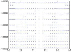
Figure 2. An example of an
inhomoge-neous mesh of the space of parameters (with 500 points). The two parameters are w=D/Randx0.
for some time T0 (in the past).
We generate a virtual population of solutions of the KPP equation, assuming Gaussian distributions on its parameters, and adding noise. We then try to recover the distributions of the parameters by a SAEM approach (using Monolix software [22]). For this we first precompute solutions of the KPP equation on a regular or non regular mesh (see Figure 2), and then run SAEM algorithm using interpolations of the precomputed values of KPP equation (instead of the genuine KPP).
As illustrated in table 1, the results are of good quality. Adding some noise deteriorates the accuracy but the results are reasonable for practical applications.
Theor E1 E2 E3
error error error
R 0.0245 0.0237 -3.3% 0.0234 -4.5% 0.0231 -5.7% D 8.64e−7 8.67e−7 0.3% 8.79e−7 1.7% 9.62e−7 11% x0 0.415 0.399 -3.9% 0.393 -5.3% 0.37 -11%
ωR 0.201 0.196 -2.5% 0.263 31% 0.253 26%
ωD 0.205 0.188 -8.3% 0.247 20% 0.395 93%
ωx0 0.254 0.244 -3.9% 0.241 -5% 0.616 143%
Table 1. Results (from Monolix) and errors for the mean parameters of the population. Col-umn E1 refers to a population without noise (see text). ColCol-umn E2 (resp. E3) refers to a population with a 5% (resp. 10%) noise. Test with homogeneous grid.
The main interest of this methodology is to tackle problem of parameters identification in complex PDE systems. The computational cost of the whole algorithm that mean generation of the mesh and SAEM com-putation, can be divided in two distinct parts: an offline time corresponding to the computation of the mesh, which can be done once and for all, and an online time corresponding to the estimation of the parameters for a given population.
In the previous example, the gain is of order 725 for the homogeneous grid and 1200 for the heterogeneous grid compared to a full computation with a whole resolution of the PDE during the SAEM algorithm.
3.4.
Conclusions
In this work we present a new method combining SAEM algorithm and a precomputation step. This method could be helpful to reduce the overall computation time when the model is very long to compute, for instance when the model is based on partial differential equations.
4.
Greedy algorithms and model reduction
In this section, we will briefly present a general method to approximate high-dimensional functions. This technique can be used in particular to solve high-dimensional partial differential equations. This section is related to a series of recent works [4–6, 16]. We also refer to the contribution of Virginie Ehrlacher to this volume for an application of this technique to eigenvalue problems.
4.1.
An introductory example
To fix the idea, let us consider the parametric problem: findu(θ, x) a real valued function solution to, for all θ∈ T,
(
−divx(a(θ, x)∇xu(θ, x)) =f(θ, x) ∀x∈ X,
u(θ, x) = 0 ∀x∈∂X. (7)
Here, x varies in subdomain X of Rd, θ is a parameter which lives inT a subset of
Rp. We assume in the
following that (θ, x)7→a(θ, x) and (θ, x)7→f(θ, x) are two real valued functions such that for almost all values of the parameterθ∈ T, the problem (7) is well posed. For example,f is inL2(T × X),ais inL∞(T × X) and is
bounded from below by a positive constant, so that there exists a unique solutionu∈L2(T, H2(X)∩H1 0(X)).
This is the setting we will consider in the following. The functional spacesH1
0(X) andH2(X) are the classical
Sobolev spaces: H1
0(X) ={v :X 7→R, v∈L2(X), |∇xv| ∈L2(X) andv = 0 on∂X } and H2(X) ={v :X 7→
R, v∈L2(X), |∇xv| ∈L2(X) and|∇2x,xv| ∈L2(X)}.
A parameter estimation problem typically writes as follows: given some observations on the functionu(θ, x), how to estimate the values ofθ∈ T ? Many approaches have been proposed to solve this inverse problem, and it is not the aim of this section to discuss them. We rather would like to explain a method to approximate the high-dimensional function (θ, x)7→u(θ, x). This approximation can then be used to solve the inverse problem, for example to provide a first guess to a deterministic optimization approach or to build a variance reduction technique in a Bayesian technique. Such an approximation is sometimes called a response surface, or a reduced order model.
The difficulty is of course that the functionsudepends on the variable (θ, x) with dimensiond+p. Standard approximation techniques based for example on tensorization of one dimensional grids lead to a huge number of degrees of freedom, since the complexity is exponential in the dimension. This is the so-called curse of dimensionality. Various approaches have been proposed to tackle this difficulty such as sparse grids techniques base [3, 24] or reduced bases methods [17, 19]. We here focus on an algorithm introduced by Ladev`eze [15], Ammar [1] and Nouy [18] that we call below the greedy algorithm. This algorithm is also sometimes called the Proper Generalized Decomposition.
4.2.
The greedy algorithm
Let us now present the greedy algorithm we are interested in. The bottom line is to approximate the function u(θ, x) as a sum of tensor products:
u(θ, x) =X k≥1
rk(θ)sk(x)
and to compute each of the terms in this sum iteratively, as the best next tensor product approximation. Depending on the problem under consideration, this best approximation is defined in various ways. This algorithm is greedy in the sense that the terms are computed iteratively and once one of them is computed, it is not modified in the following iterations. For simplicity, we consider the tensor product of only two functions (rk(θ) andsk(x)) but the algorithm equally applies to a tensor product of more than two functions. For example, if the parametric space is high-dimensional (namely if pis large), one could think of using a decomposition of the formu(θ, x) =P
In the specific example (7) above, the algorithm writes as follows: iterate onK≥0
(rK+1, sK+1)∈ argmin
r∈L2(T),s∈H1 0(X)
E
K
X
k=1
rk(θ)sk(x) +r(θ)s(x)
!
(8)
where
E(v) = 1 2 Z
T ×X
a(θ, x)|∇xv|2dθ dx−
Z
T ×X
f(θ, x)v(θ, x)dθ dx
is the energy functional associated to (7), defined forv∈L2(T, H1
0(X)). The energy functionalE has a unique
minimum, which is characterized by the Euler equations (7). The idea underlying the algorithm (8) is that at each iteration, the best tensor product minimizing E is chosen.
In practice, to solve (8), one actually considers the Euler Lagrange equations associated to (8), which are: iterate onK≥0, findrK+1∈L2(T) andsK+1∈H01(X) such that, for allδr∈L2(T) andδs∈H01(X)
Z
T ×X
a(θ, x)∇x(uK(θ, x) +rK+1(θ)sK+1(x))· ∇x(rK+1(θ)δs(x) +δr(θ)sK+1(x))dθ dx
= Z
T ×X
f(θ, x)(rK+1(θ)δs(x) +δr(θ)sK+1(x))dθ dx
(9)
where, for the ease of notation, we introduced
uK(θ, x) = K
X
k=1
rk(θ)sk(x). (10)
The problem (9) is the weak form of the problem:
−divx
Z
T
a(θ, x)(rK+1(θ))2dθ
∇xsK+1(x)
= Z
T
rK+1(θ) (f(θ, x) + divx(a(θ, x)∇xuK(θ, x))) dθ,
rK+1(θ) Z
X
a(θ, x)|∇xsK+1|2dx=
Z
X
(f(θ, x) + divx(a(θ, x)∇xuK(θ, x)))sK+1(x)dx,
(11) where the first equation is an elliptic problem onsK+1 (for a fixed functionrK+1) with homogeneous Dirichlet
boundary conditions, and the second equation gives rK+1 (for a fixed function sK+1). Two remarks are in
order. First, it is obvious from the formulation (11) that the problem defining the couple (rK+1, sK+1) is
nonlinear: starting from the linear problem (7), we end up with the nonlinear problem (11). This is because the space of tensor products is not a linear space. Second, if we assume that the dataaand f admit a separated representation of the form a(θ, x) = P
k≥1r
a k(θ)s
a
k(x) and f(θ, x) =
P
k≥1r
f k(θ)s
f
k(x), then, all the integrals involved in (11) are either integrals overT or overX, using the Fubini’s theorem: there is no integral over the product spaceT × X. In practice, (11) is typically solved by a fixed point algorithm.
Notice that compared to the original problem which was with complexity Nd+p (ifN denotes the number of degrees of freedom per dimension), the new formulation is a sequence of problems with a much smaller complexity, namelyNd+Np. This comes at a price: the nonlinearity of (11).
4.3.
Convergence
The algorithm (8) is at the interface between two approximation techniques:
(ii) the greedy algorithms developed in the field of nonlinear approximation, to approximate a function as a sum of elements of adictionary(which is not necessarily the set of tensor products), see [23]. In the algorithm (8), we both use tensor products to approximate the solution (as in item (i) above) and a greedy technique to compute the terms of the sum (as in item (ii) above).
The convergence of the algorithm can actually be deduced from general results on the convergence of greedy algorithms [8, 16].
Theorem 1. Let us consider the algorithm (8)and the functionuK defined by (10). The following convergence result holds: lim
K→∞kuK−ukL2(T,H
1
0(X)) = 0.Moreover, if u∈ L
1 where the Banach space L1⊂L2(T, H1 0(X))
is defined as the set of functions with finiteprojective norms
L1=
u(θ, x) =X k≥0
ckrk(θ)sk(x), s.t. rk∈L2(T), sk∈H01(X)),krk(θ)sk(x)kL2(T,H1
0(X))= 1 and X
k≥0
|ck|<∞
,
then there exists C >0 (which depends onu) such that, for all positive K,kuK−ukL2(T,H1
0(X))≤CK
−1/6.
The convergence rate can be improved to−1/2 using an orthogonal version of the algorithm. The theorem also holds for tensor products of more than two functions.
This result essentially tells us that the algorithm is safe: it is converging. On the other hand, the convergence rate is rather slow. In practice, one typically observes that the convergence is exponential for small values of K, and then slows down.
4.4.
Extensions and open questions
The prototypical example (7) enjoys two specific properties: it islinearandsymmetric. In [4], we were able to generalize the convergence result to nonlinear problems, which are still defined as the minimum of some functional. In this case however, we have no convergence rates. In [6], we investigated various techniques to generalize the approach to linear but non-symmetric problems, which are thus not simply associated to an energy minimization problem: there is up to now no satisfactory technique to treat non-symmetric problems. We have also on-going works on parametric eigenvalue problems.
Generally speaking, the main question which seems difficult to attack is the following: if the solution to the original problem admits a separated representation (sum of tensor product functions) with a small number of terms, will the greedy algorithms be able to approximate efficiently this function ? There has been very encouraging results in that direction for some greedy algorithms recently [2] but it is unclear if they can be extended to our setting.
References
[1] A. Ammar, B. Mokdad, F. Chinesta, and R. Keunings. A new family of solvers for some classes of multidimensional partial differential equations encountered in kinetic theory modeling of complex fluids.J. Non-Newtonian Fluid Mech., 139:153–176, 2006.
[2] P. Binev, A. Cohen, R. Dahmen, W.and DeVore, G. Petrova, and P. Wojtaszczyk. Convergence rates for greedy algorithms in the reduced basis method.SIAM J. Math. Anal., 43:1457–1472, 2011.
[3] H.-J. Bungartz and M. Griebel. Sparse grids.Acta Numer., 13:147–269, 2004.
[4] E. Canc`es, V. Ehrlacher, and T. Leli`evre. Convergence of a greedy algorithm for high-dimensional convex nonlinear problems.
Math. Models and Methods in Applied Sciences, 21(12):2433–2467, 2011.
[5] E. Canc`es, V. Ehrlacher, and T. Leli`evre. Greedy algorithms for high-dimensional eigenvalue problems, 2012.
http://hal.archives-ouvertes.fr/hal-00809855.
[6] E. Canc`es, V. Ehrlacher, and T. Leli`evre. Greedy algorithms for high-dimensional non-symmetric linear problems, 2012.
http://hal.archives-ouvertes.fr/hal-00745611.
[7] B. Delyon, M. Lavielle, and E. Moulines. Convergence of a stochastic approximation version of the EM algorithm.The Annals of Statistics, 27(1):94–128, 1999.
[9] S.V. Dolgov, B.N. Khoromskij, and I. Oseledets. Fast solution of multi-dimensional parabolic problems in the TT/QTT formats with initial application to the fokker-planck equation.SIAM J. Sci. Comp., 34(6):3016–3038, 2012.
[10] M. Doumic, M. Hoffmann, N. Krell, and L. Robert. Statistical estimation of a growth-fragmentation model observed on a genealogical tree.arXiv:1210.3240, 2013.
[11] M. Doumic, M. Hoffmann, P. Reynaud-Bouret, and V. Rivoirard. Nonparametric estimation of the division rate of a size-structured population.SIAM Journal on Numerical Analysis, 50:925–950, 2012.
[12] M. Doumic, B. Perthame, and J. Zubelli. Numerical solution of an inverse problem in size-structured population dynamics.
Inverse Problems, 25:25pp, 2009.
[13] W. Hackbusch.Tensor spaces and numerical tensor calculus. Springer, 2012.
[14] E. Kuhn and M. Lavielle. Maximum likelihood estimation in nonlinear mixed effects models. Computational Statistics and Data Analysis, 49(4):1020–1038, 2005.
[15] P. Ladev`eze. Nonlinear computational structural mechanics: new approaches and non-incremental methods of calculation. Springer, 1999.
[16] C. Le Bris, T. Leli`evre, and Y. Maday. Results and questions on a nonlinear approximation approach for solving high-dimensional partial differential equations.Constructive Approximation, 30(3):621–651, 2009.
[17] L. Machiels, Y. Maday, and A.T. Patera. Output bounds for reduced-order approximations of elliptic partial differential equations.Comput. Methods Appl. Mech. Engrg., 190(26-27):3413–3426, 2001.
[18] A. Nouy. A generalized spectral decomposition technique to solve a class of linear stochastic partial differential equations.
Comput. Methods Appl. Mech. Engrg., 196:4521–4537, 2007.
[19] C. Prud’homme, D. Rovas, K. Veroy, Y. Maday, A.T. Patera, and G. Turinici. Reliable real-time solution of parametrized partial differential equations: Reduced-basis output bounds methods.Journal of Fluids Engineering, 124(1):70–80, 2002. [20] N. Rachdi, J.-C. Fort, and T. Klein. Stochastic inverse problem with noisy simulator—application to aeronautical model.Ann.
Fac. Sci. Toulouse Math. (6), 21(3):593–622, 2012.
[21] N. Rachdi, J.-C. Fort, and T. Klein. Risk bounds for new m-estimation problems.ESAIM: Probability and Statistics, eFirst, 8 2013.
[22] Monolix Team. The Monolix software, Version 4.1.2. Analysis of mixed effects models. LIXOFT and INRIA, http://www.lixoft.com/, March 2012.
[23] V.N. Temlyakov. Greedy approximation.Acta Numerica, 17:235–409, 2008.