The marginalized particle filter – analysis, applications and generalizations

Christophe Andrieu & Dan Crisan, Editors DOI: 10.1051/proc:071908

THE MARGINALIZED PARTICLE FILTER –

ANALYSIS, APPLICATIONS AND GENERALIZATIONS

Thomas B. Sch¨

on, Rickard Karlsson and Fredrik Gustafsson

Abstract. The marginalized particle filter is a powerful combination of the particle filter and the Kalman filter, which can be used when the underlying model contains a linear sub-structure, subject to Gaussian noise. This paper outlines the marginalized particle filter and very briefly hint at pos-sible generalizations, giving rise to a larger family of marginalized nonlinear filters. Furthermore, we analyze several properties of the marginalized particle filter, including its ability to reduce variance and its computational complexity. Finally, we provide an introduction to various applications of the marginalized particle filter.

1.

Introduction

Many problems in for instance positioning and target tracking can be cast as nonlinear state estimation problems, where the uncertainty in the process model and/or in the measurement model may be non-Gaussian. Such a general model can be formulated according to

x_t+1 =f(x_t, u_t) +w_t, (1a)

y_t=h(xt) +et, (1b)

with state variable xt ∈Rm, input signal ut and measurements Yt ={yi}ti=1, with knownprobability density function (PDF) for the process noisepw(w) and the measurement noise pe(e). Hence, traditional estimation methods based on the Kalman filter (KF) [19, 20], or linearized version thereof, do not always provide good performance. Over the past 40 years there has been several suggestions on how to tackle the problem of estimating the states in (1). An appealing solution is provided by the particle filter (PF) [9, 17, 30], which allows for a systematic treatment of both nonlinearities and non-Gaussian noise. However, due to the inherent computational complexity of the particle filter, real-time issues arise in many applications when the sampling rate is high. Furthermore, the particle filter only works for moderate state dimensions, when the state dimension is large, something else is required. If the model includes a sub-structure with linear equations, subject to Gaussian noise, it is possible to exploit this in the estimator. Here, this method is referred to as themarginalized particle filter (MPF), it is also known as the Rao-Blackwellized particle filter, see for instance [2,3,6,9,10,33]. The MPF is a combination of the standard particle filter and the Kalman filter. It is a well known fact that in some cases it is possible to obtain better estimates, i.e., estimates with reduced variance, using the marginalized particle filter instead of using the standard particle filter [12].

1 _{Division of Automatic Control} Department of Electrical Engineering Link¨oping University, Sweden SE–581 83 Link¨oping, Sweden

c

EDP Sciences, SMAI 2007

It is the linear, Gaussian sub-structure that opens up for the use of the marginalized particle filter. Hence, it is a structural property of the underlying model. It is interesting to note that this property can be exploited in combination with other nonlinear filters as well, resulting in a rather general class of filters, which we will refer to asmarginalized nonlinear filters (MNLF).

The aim of this paper is to introduce the the marginalized particle filter and very briefly hint at possible extensions. We will also provide an overview of some of the applications where the marginalized particle filter has been successfully applied. Since we cannot cover all the details in this paper references to more detailed treatments are provided.

2.

Marginalized Nonlinear Filters

The aim of recursively estimating the filtering density p(x_t|Y_t) can be accomplished using the standard particle filter. However, if there is a linear sub-structure, subject to Gaussian noise, present in the model this can be exploited to obtain better estimates and possibly reduce the computational demand as well. This, together with the fact that the standard particle filter might be prohibited due to a too high state dimension, constitutes the motivation underlying the marginalized nonlinear filters.

2.1.

Representation

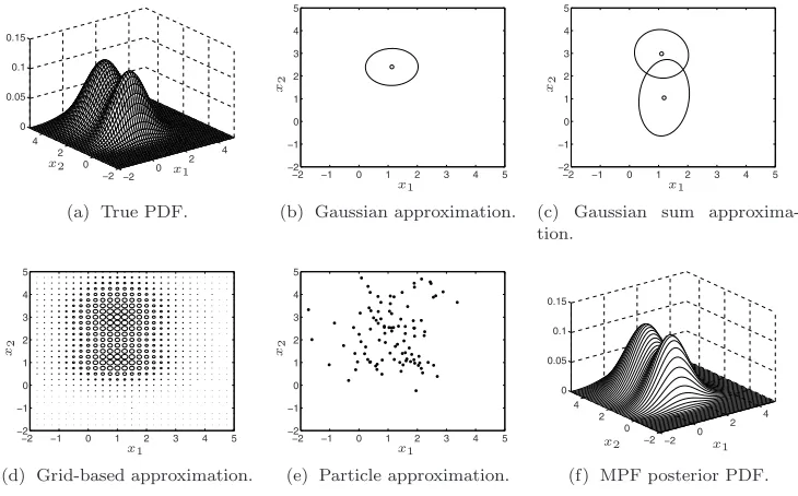
The task of nonlinear filtering can be split into two parts: representation of the filtering probability density function and propagation of this density during the time and measurement update stages. Figure 1 illustrates different representations of the filtering density for a two-dimensional example (similar to the example used in Section 4). Theextended Kalman filter(EKF) [1, 19], can be interpreted as using one Gaussian distribution for representation and the propagation is performed according to a linearized model. TheGaussian sum filter[1,35] extends the EKF to be able to represent multi-modal distributions, still with an approximate propagation.

−2 0 2 4 −2 0 2 4 0 0.05 0.1 0.15 x1 x2

(a) True PDF.

−2 −1 0 1 2 3 4 5 −2 −1 0 1 2 3 4 5 x1 x2

(b) Gaussian approximation.

−2 −1 0 1 2 3 4 5 −2 −1 0 1 2 3 4 5 x1 x2

(c) Gaussian sum approxima-tion.

−2 −1 0 1 2 3 4 5 −2 −1 0 1 2 3 4 5 x1 x2

(d) Grid-based approximation.

−2 −1 0 1 2 3 4 5 −2 −1 0 1 2 3 4 5 x1 x2

(e) Particle approximation.

−2 0 2 4 −2 0 2 4 0 0.05 0.1 0.15 x1 x2

(f) MPF posterior PDF.

Figure 1. _{True probability density function and different approximate representations, in}

Figure 1(d)–(f) illustrates numerical approaches where the exact nonlinear relations present in the model are used for propagation. Thepoint-mass filter(grid-based approximation) [4] employ a regular grid, where the grid weight is proportional to the posterior. Theparticle filter(PF), [17] represents the posterior by a stochastic grid in form of a set of samples, where all particles (samples) have the same weight. Finally, themarginalized particle filter (MPF) uses a stochastic grid for some of the states, and Gaussian distributions for the rest. That is, the MPF can be interpreted as a particle representation for a subspace of the state space, where each particle has an associated Gaussian distribution for the remaining state dimensions, Figure 1(f). It will be demonstrated that an exact nonlinear propagation is still possible if there is a linear sub-structure in the model. An important model class has the property that the (co-)variance is the same for all particles, which simplifies computations significantly.

2.2.

Model

Consider a state vectorx_t, which can be partitioned according to

x_t=

xn t xl t

, (2)

where xl_t denotes the linear states and xn_t denotes the nonlinear states, in the dynamics and measurement relation. A rather general model with the properties discussed above is given by

xn

t+1=ftn(xnt, kt)+An_t(xn_t, kt)xl_t+Gn_t(xn_t, kt)w_tn, (3a)

xl

t+1=ftl(xnt, kt) +Alt(xnt, kt)xlt+Glt(xnt, kt)wlt, (3b) y_t=h_t(xn_t, k_t) +C_t(xn_t, k_t)xl_t+e_t, (3c)

where k_t is used to denote a discrete mode parameter. Furthermore, the state noise is assumed white and Gaussian distributed with

w_t=

wn t wl t

∼ N(0, Q_t), Q_t=

Qn

t Qlnt

(Qln_t )T Ql_t

. (3d)

The measurement noise is assumed white and Gaussian distributed according to

e_t∼ N(0, R_t). (3e)

Furthermore,xl₀is Gaussian,

xl

0∼ N(¯x0,P¯0). (3f)

Finally, the density of xn₀ can be arbitrary, but it is assumed known. More specifically, conditioned on the nonlinear state variables and the discrete mode parameters there is a linear sub-structure, subject to Gaussian noise available in (3), given by (3b).

Bayesian estimation methods, such as the particle filter, provide estimates of the filtering density function

p(x_t, k_t|Y_t). By employing the fact

p(xl_t,X_tn, K_t|Y_t) =p(x_tl|X_tn, K_t, Y_t)p(X_tn, K_t|Y_t) =p(xl_t|X_tn, K_t, Y_t)p(X_tn|K_t, Y_t)p(K_t|Y_t), (4)

• A Kalman filter operating on the conditionally linear, Gaussian model (3) provides an estimate of

p(xl_t|X_tn, K_t, Y_t). Note that, conditioned on that the nonlinear state sequence X_tn and discrete mode sequenceK_tmodel (3) is a linear, Gaussian model.

• A marginalized nonlinear filter (e.g., PF, PMF, Gaussian sum filters, UKF) is designed for a fixed mode sequence.

• A pruning or merging scheme (IMM, AFMM) for the exponentially increasing number of mode se-quences, see Chapter 10 in [18].

It is very important to note that the three sub-problems mentioned above are all coupled, for example, the result from the nonlinear filter at time t is used by the Kalman filters at timet. This is further explained in the subsequent section.

3.

Marginalized Particle Filter

In the MPF the marginalized nonlinear filter is given by a particle filter. The present discussion assumes that there are no discrete modes k_t present. This is just to make the presentation more accessible.

3.1.

Algorithm

Similarly to (4) the filtering density function p(x_t|Y_t) is given by (assuming no discrete modes)

p(xl_t, X_tn|Yt) =p(xl_t|X_tn, Yt)p(X_tn|Yt). (5)

Using this expression the problem can be put in a form that is suitable for the MPF framework, i.e., to analytically marginalize out the linear state variables from p(x_t|Y_t). Note that p(xl_t|X_tn, Y_t) is analytically tractable, sinceX_tn is given by the particle filter. Hence, the underlying model is conditionally linear-Gaussian, and the PDF can be computed from the Kalman filter. Furthermore, an estimate ofp(xn_t|Y_t) is provided by the particle filter, more specifically, it is given by

p(xn_t|Y_t) =

N

i=1

˜

ω_tδ(xn_t −xn,_t (i)). (6)

Hence, the resulting PDF estimate is given by

p(xt|Yt) =

N

i=1

˜

ω_tδ(xn_t −x_tn,(i))N(x_tl; ˆxl,_t|(_ti), P_t(_|i_t)), (7)

motivating the fact that the MPF provides an estimate of the PDF that is a mix of a parametric and an unparametric estimate. That is a mix of a parametric distribution from the Gaussian family and a nonparametric distribution represented by samples. Another name for the MPF is the Rao-Blackwellized particle filter, and it has been known for quite some time, see e.g., [2, 5, 6, 10, 12, 12, 29, 33]. If the same numbers of particles are used in the standard PF and the MPF, the latter will provide estimates of better or at least the same quality. Intuitively this makes sense, since the dimension ofp(xn_t|Yt) is smaller than the dimension ofp(xt|Yt), implying that the particles occupy a lower dimensional space. Furthermore, the optimal algorithm is used to estimate the linear state variables. For a detailed discussion regarding the improved accuracy of the estimates, see, e.g., [11, 12].

Algorithm 1Marginalized particle filter

(1) Initialization: For i = 1, . . . , N, initialize the particles, x₀n,_|−(i₁) ∼ p_xn

0(xn0) and set {x

l,(i)

0|−1, P0(|−i)1} =

{x¯l₀,P¯₀}. Sett:= 0.

(2) PF measurement update: Fori= 1, . . . , N, evaluate the importance weights

ω_t(i)=p

y_t|X_tn,(i), Y_t−1, (8)

and normalize ˜ω(_ti)=ω_t(i)/N_j=1ω_t(j). (3) ResampleN particles, with replacement,

P rxn,_t|t(i)=xn,_t|t(₋j)₁

= ˜ω_t(j).

(4) PF time update and KF:

(a) Kalman filter measurement update:

ˆ

xl

t|t= ˆxlt|t−1+Kt

y_t−h_t−C_txˆl_t|t−1

, (9a)

P_t|t=P_t|t−1−K_tM_tK_tT, (9b)

M_t=CtPt|t−1CtT+Rt, (9c)

K_t=P_t|t−1C_tTM_t−1. (9d)

(b) PF time update (prediction): Fori= 1, . . . , N, predict new particles,

xn,_t+1(i)_|t∼pxn

t+1|t|Xtn,(i), Yt

. (c) Kalman filter time update:

ˆ

xl

t+1|t= ¯Altxˆlt|t+Glt(Qlnt )T(GntQtn)−1zt+ftl

+L_t

z_t−An txˆlt|t

, (10a)

P_t+1|t= ¯Al_tP_t|t( ¯Al_t)T +Gl_tQ¯l_t(Gl_t)T −L_tN_tLT_t, (10b)

N_t=An_tP_t|t(An_t)T +Gn_tQn_t(Gn_t)T, (10c)

L_t= ¯Al_tP_t|t(An_t)TN_t−1, (10d)

where

z_t=xn_t+1−f_tn, (11a)

¯

Al

t=Alt−Glt(Qlnt )T(GntQnt)−1Ant, (11b)

¯

Ql

t=Qlt−(Qlnt )T(Qnt)−1Qlnt . (11c)

(5) Sett:=t+ 1 and iterate from step 2.

The estimates, as expected means, of the state variables and their covariances are given below.

ˆ

xn t|t=

N

i=1

˜

ω(_ti)xˆn,_t|t(i), (12a)

ˆ

Pn t|t=

N

i=1

˜

ω_t(i)xˆ_tn,_|t(i)−xˆ_tn_|t xˆ_tn,_|t(i)−xˆn_t|t

_T

, (12b)

ˆ

xl t|t=

N

i=1

˜

ω(_ti)xˆl,_t|(_ti), (12c)

ˆ

Pl t|t=

N

i=1

˜

ω(_ti)

P_t(_|i_t)+

ˆ

x_tl,_|(_ti)−xˆl_t|t xˆl,_t|(_ti)−xˆl_t|t

_T

, (12d)

where{ω˜_t(i)}N_i=1 are the normalized importance weights, provided by step 2 in Algorithm 1.

3.2.

Analysis

In this section, several properties important in the practical application of the MPF are analyzed. First, the variance reduction inherent using the Rao-Blackwellization idea is explained. Second, the computational burden of the MPF is analyzed in detail. Note that this analysis is not generally applicable, it has to be performed on a case by case basis. However, the approach briefly outlined in Section 3.2.2 below can always be used.

3.2.1. Variance Reduction

The variance of a function or estimatorg(U, V), depending on two random variables,U andV can be written as

Var{g(U, V)}=Var{E{g(U, V)|V}}+ E{Var{g(U, V)|V}}. (13)

Hence, in principle, the conditional inequality

VarE{g(x_tl, X_tn)|X_tn}≤Varg(xl_t, X_tn), (14)

can be employed. In the current MPF setup, U and V are represented by the linear and nonlinear states, respectively. This is sometimes referred to as Rao-Blackwellization, see, e.g., [31] and it is the basic part that improves performance using the marginalization idea. Note that for the variance reduction to be significant, the left hand side in (14) has to be significantly smaller than the right hand side. In other words, the term

EVar{g(xl_t, X_tn)|X_tn} (15)

has to be large. That is, the expectation of the conditional variance of the corresponding Kalman filter has to be large. In order to make this a bit clearer, letg(xl_t, X_tn) =xl_t, implying that (15) reads

VarE{xl_t|X_tn}≤Var{xl_t} (16)

This shows that the variance of the linear part is always smaller for the MPF then for the PF. The difference is the expected variance term,

This states that the improvement in the quality of the estimate is given by the term E{P_ti_|t}. That is, the Kalman filter covarianceP_t|t is a good indicator of how much that has been gained in using the MPF instead of the PF.

3.2.2. Computational Complexity

In discussing the use of the MPF it is sometimes better to partition the state vector into one part that is estimated using the PF xp_t ∈ Rp and one part that is estimated using the KF xk_t ∈ Rk. Obviously all the nonlinear statesxn_t are included inxp_t. However, we could also choose to include some of the linear states there as well. Under the assumption of linear dynamics, this notation allows us to write (3) according to

xp_t+1=Ap_txp_t +Ak_tx_tk+wp_t, w_tp ∼ N(0, Qp_t), (18a)

xk

t+1=Ftpxpt+Ftkxkt+wkt, wkt ∼ N(0, Qkt), (18b) y_t=h_t(xp_t) +C_tx_tk+e_t, e_t∼ N(0, R_t). (18c)

First, the case Ct = 0 is discussed. For instance, the first instruction P_t|t(Ak_t)T corresponds to multiplying

P_t|t ∈ Rk×k _{with (A}k

t)T ∈ Rk×p, which requires pk2 multiplications and (k−1)kpadditions [16]. The total

equivalent flop (EF)1complexity is derived by [24],

C(p, k, N)≈4pk2+ 8kp2+4 3p

3_{+ 5k}3_{−5kp+ 2p}2_{+ (6kp+ 4p}2_{+ 2k}2_+p−k+pc

3+c1+c2)N. (19)

Here, the coefficientc₁has been used for the calculation of the Gaussian likelihood,c₂for the resampling andc₃ for the random number complexity. Note that, whenC_t= 0 the same covariance matrix is used for all Kalman filters, which significantly reduce the computational complexity.

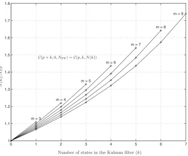
By requiringC(p+k,0, NPF) =C(p, k, N(k)), whereNPF corresponds to the number of particles used in the standard PF we can solve for N(k). This gives the number of particles N(k) that can be used by the MPF in order to obtain the same computational complexity as if the standard PF had been used for all states. In Figure 2 the ratioN(k)/NPF is plotted for systems withm= 3, . . . ,9 states.

Hence, using Figure 2 it is possible to directly find out how much there is to gain in using the MPF from a computational complexity point of view. The figure also shows that the computational complexity is always reduced when the MPF can be used instead of the standard PF. Furthermore, as previously mentioned, the quality of the estimates will improve or remain the same when the MPF is used [12].

Second, ifC_t= 0, the Riccati recursions have to be evaluated separately for each particle. This results in a significantly increased computational complexity. Hence, different covariance matrices have to be used for each Kalman filter, implying that (19) has to be modified. Approximately the complexity is given by [24],

C(p, k, N)≈(6kp+ 4p2+ 2k2+p−k+pc₃+c₁+c₂+ 4pk2+ 8kp2+4 3p

3_{+ 5k}3_{−5kp+ 2p}2_+k3_{)N. (20)}

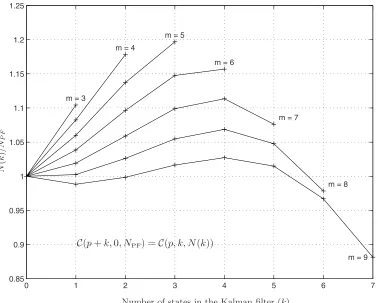
In Figure 3 the ratioN(k)/NP F is plotted for systems withm= 3, . . . ,9 states. For systems with few states the MPF is more efficient than the standard PF. However, for systems with more states, where most of the states are marginalized the standard PF becomes more efficient than the MPF. This is due to the Riccati recursions mentioned above.

1_{The EF complexity for an operation is defined as the number of flops that result in the same computational time as the}

0 1 2 3 4 5 6 7 1

1.1 1.2 1.3 1.4 1.5 1.6 1.7 1.8

m = 3

m = 4

m = 5

m = 6

m = 7

m = 8

m = 9

N

(

k

)

/N

PF

Number of states in the Kalman filter (k) C(p+k,0, N_PF) =C(p, k, N(k))

Figure 2. RatioN(k)/N_PF for systems withm= 3, . . . ,9 states andC_t= 0,n= 2 is shown.

It is apparent the MPF can use more particles for a given computational complexity, when compared to the standard PF.

4.

Illustrating Example

The aim here is to illustrate how the MPF works using the following nonlinear stochastic system.

xn

t+1=xltxnt +wnt, (21a)

xl

t+1=xlt+wtl, (21b)

y_t= 0.2(xn_t)2+e_t, (21c)

where the noise is assumed white and Gaussian according to

w_t=

wn t wl t

∼ N

0 0

,

0.25 0 0 10−4

, (21d)

e_t∼ N(0,1). (21e)

The initial state x₀ is given by

x₀∼ N

0.1 0.99

,

16 0

0 10−3

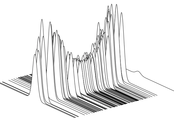
This system was used in [38], where it illustrated grid-based (point-mass) filters. Obviously, the states can be estimated by applying the standard particle filter to the entire state vector. However, a better solution is to exploit the conditionally linear, Gaussian sub-structure that is present in (21). The nonlinear process xn_t is a first-order AR process, where the linear process xl_t is the time-varying parameter. The linear, Gaussian sub-structure is used by the MPF and the resulting filtering density function at time 10, p(x₁₀|Y₁₀) is given in Figure 4 (for a particular realization). In this example 2000 particles were used, but only 100 of them are plotted in Figure 4 in order to obtain a clearer illustration of the result. The figure illustrates the fact that the MPF is a combination of the KF and the PF. The density functions for the linear states are provided by the Kalman filters, which is evident from the fact that the marginal densitiesp(xl,_t(i)|Y_t) are given by Gaussian densities. Furthermore, the nonlinear state estimates are provided by the PF. Hence, the linear states are given by a parametric estimator (KF), whereas the nonlinear states are given by a nonparametric estimator (PF). In this context the MPF can be viewed as a combination of a parametric and an unparametric estimator.

5.

Application Overview

Two important areas where the MPF has been successfully applied are GPS-freepositioning, where the aim is to estimate the own platform’s position and target tracking, where the state of an unknown, observed target

0 1 2 3 4 5 6 7

0.85 0.9 0.95 1 1.05 1.1 1.15 1.2 1.25

m = 3

m = 4

m = 5

m = 6

m = 7

m = 8

m = 9

N

(

k

)

/N

PF

Number of states in the Kalman filter (k) C(p+k,0, NPF) =C(p, k, N(k))

Figure 3. RatioN(k)/N_PF for systems withm= 3, . . . ,9 states andC_t= 0,n= 2 is shown.

Figure 4. The estimated filter PDF for system (21) at time 10,p(x₁₀|Y₁₀) using the MPF. It is

instructive to see that the linear statexl₁₀is estimated by Gaussian densities (from the Kalman filter) and position along the nonlinear statexn₁₀is given by a particles (from the particle filter). Note that only a subset of particles have been plotted, in order to make the illustration clear.

is estimated from measurements. These applications also represent typical examples where sensor fusion tech-niques are important. The MPF provides an efficient way to incorporate both linear and nonlinear measurement relations. A more detailed overview of some of our MPF applications is provided [34]. In simultaneous local-ization and mapping (SLAM) applications, where the map information is built up from measurement data, the MPF is one of the key techniques for fast real-time applications, see for instance [37]. In SLAM applications the resulting algorithm is sometimes refered to as FastSLAM.

Here is a list of some MPF applications:

Positioning and map applications:

• Underwater terrain-aided positioning [21, 23] • Aircraft terrain-aided positioning [33] • Automotive map-aided positioning [36] • GPS navigation [15]

• Simultaneous Localization and Mapping (SLAM)[13, 27, 28, 37]

Target tracking applications:

• Radar target tracking [34]

Other applications:

• Communication applications [7, 39] • System identification [8, 25, 26, 32] • Audio applications [3].

Acknowledgment

This work was supported by VINNOVA’s Center of Excellence ISIS (Information Systems for Industrial Control and Supervision), and by the Swedish Research Council (VR).

References

[1] B. D. O. Anderson and J. B. Moore.Optimal Filtering. Information and system science series. Prentice Hall, Englewood Cliffs, NJ, USA, 1979.

[2] C. Andrieu and A. Doucet. Particle filtering for partially observed Gaussian state space models.Journal of the Royal Statistical Society, 64(4):827–836, 2002.

[3] C. Andrieu and S. J. Godsill. A particle filter for model based audio source separation. In Proceedings of the International Workshop on Independent Component Analysis and Blind Signal Separation (ICA 2000), Helsinki, Finland, June 2000. [4] N. Bergman.Recursive Bayesian Estimation: Navigation and Tracking Applications. Phd thesis No 579, Link¨oping Studies

in Science and Technology, SE-581 83 Link¨oping, Sweden, May 1999.

[5] G. Casella and C. P. Robert. Rao-Blackwellisation of sampling schemes.Biometrika, 83(1):81–94, 1996. [6] R. Chen and J. S. Liu. Mixture Kalman filters.Journal of the Royal Statistical Society, 62(3):493–508, 2000.

[7] R. Chen, X. Wang, and J. S. Liu. Adaptive joint detection in flat-fading channels via mixture Kalman filtering.IEEE Trans-actions on Information Theory, 46(6):2079–2094, 2000.

[8] M. J. Daly, J. P. Reilly, and M. R. Morelande. Rao-Blackwellised particle filtering for blind system identification. InProceedings of the IEEE International Conference on Acoustics, Speech, and Signal Processing, Philadelphia, PA, USA, Mar. 2005. [9] A. Doucet, N. de Freitas, and N. Gordon, editors.Sequential Monte Carlo Methods in Practice. Springer Verlag, New York,

USA, 2001.

[10] A. Doucet, S. J. Godsill, and C. Andrieu. On sequential Monte Carlo sampling methods for Bayesian filtering.Statistics and Computing, 10(3):197–208, 2000.

[11] A. Doucet, N. Gordon, and V. Krishnamurthy. Particle filters for state estimation of jump Markov linear systems. Technical Re-port CUED/F-INFENG/TR 359, Signal Processing Group, Department of Engineering, University of Cambridge, Trupington street, CB2 1PZ Cambridge, 1999.

[12] A. Doucet, N. Gordon, and V. Krishnamurthy. Particle filters for state estimation of jump Markov linear systems. IEEE Transactions on Signal Processing, 49(3):613–624, 2001.

[13] E. Eade and T. Drummond. Scalable monocular SLAM. InProceedings of IEEE Computer Society Conference on Computer Vision and Pattern Recognition (CVPR), pages 469–476, New York, NY, USA, June 2006.

[14] A. Eidehall, T. B. Sch¨on, and F. Gustafsson. The marginalized particle filter for automotive tracking applications. InProceedings of the IEEE Intelligent Vehicle Symposium, pages 369–374, Las Vegas, USA, June 2005.

[15] A. Giremus and J. Y. Tourneret. Joint detection/estimation of multipath effects for the global positioning system. InProceedings of IEEE International Conference on Acoustics, Speech, and Signal Processing, volume 4, pages 17–20, Philadelphia, PA, USA, Mar. 2005.

[16] G. H. Golub and C. F. Van Loan.Matrix Computations. John Hopkins University Press, Baltimore, third edition, 1996. [17] N. J. Gordon, D. J. Salmond, and A. F. M. Smith. Novel approach to nonlinear/non-Gaussian Bayesian state estimation. In

IEE Proceedings on Radar and Signal Processing, volume 140, pages 107–113, 1993.

[18] F. Gustafsson.Adaptive Filtering and Change Detection. John Wiley & Sons, New York, USA, 2000.

[19] T. Kailath, A. H. Sayed, and B. Hassibi.Linear Estimation. Information and System Sciences Series. Prentice Hall, Upper Saddle River, NJ, USA, 2000.

[20] R. E. Kalman. A new approach to linear filtering and prediction problems. Transactions of the ASME, Journal of Basic Engineering, 82:35–45, 1960.

[21] R. Karlsson and F. Gustafsson. Particle filter for underwater navigation. InProceedings of the Statistical Signal Processing Workshop, pages 509–512, St. Louis, MO, USA, Sept. 2003.

[23] R. Karlsson and F. Gustafsson. Bayesian surface and underwater navigation.IEEE Transactions on Signal Processing, 2006. Accepted for publication.

[24] R. Karlsson, T. Sch¨on, and F. Gustafsson. Complexity analysis of the marginalized particle filter.IEEE Transactions on Signal Processing, 53(11):4408–4411, Nov. 2005.

[25] P. Li, R. Goodall, and V. Kadirkamanathan. Parameter estimation of railway vehicle dynamic model using Rao-Blackwellised particle filter. InProceedings of the European Control Conference, Cambridge, UK, Sept. 2003.

[26] P. Li, R. Goodall, and V. Kadirkamanathan. Estimation of parameters in a linear state space model using Rao-Blackwellised particle filter.IEE Proceedings - Control Theory and Applications, 151(6):727–738, Nov. 2004.

[27] M. Montemerlo, S. Thrun, D. Koller, and B. Wegbreit. FastSLAM a factored solution to the simultaneous localization and mapping problem. InProceedings of the AAAI National Comference on Artificial Intelligence, Edmonton, Canada, 2002. [28] M. Montemerlo, S. Thrun, D. Koller, and B. Wegbreit. FastSLAM 2.0: An improved particle filtering algorithm for simultaneous

localization and mapping that provably converges. InProceedings of the Sixteenth International Joint Conference on Artificial Intelligence (IJCAI), Acapulco, Mexico, 2003.

[29] P.-J. Nordlund.Sequential Monte Carlo Filters and Integrated Navigation. Licentiate Thesis No 945, Department of Electrical Engineering, Link¨oping University, Sweden, 2002.

[30] B. Ristic, S. Arulampalam, and N. Gordon.Beyond the Kalman Filter: particle filters for tracking applications. Artech House, London, UK, 2004.

[31] C. P. Robert and G. Casella.Monte Carlo Statistical Methods. Springer texts in statistics. Springer, New York, 1999. [32] T. Sch¨on and F. Gustafsson. Particle filters for system identification of state-space models linear in either parameters or states.

InProceedings of the 13th IFAC Symposium on System Identification, pages 1287–1292, Rotterdam, The Netherlands, Sept. 2003.

[33] T. Sch¨on, F. Gustafsson, and P.-J. Nordlund. Marginalized particle filters for mixed linear/nonlinear state-space models.IEEE Transactions on Signal Processing, 53(7):2279–2289, July 2005.

[34] T. B. Sch¨on, R. Karlsson, and F. Gustafsson. The marginalized particle filter in practice. InProceedings of IEEE Aerospace Conference, Big Sky, MT, USA, Mar. 2006.

[35] H. W. Sorenson and D. L. Alspach. Recursive Bayesian estimation using Gaussian sum.Automatica, 7:465–479, 1971. [36] N. Svenz´en. Real time implementation of map aided positioning using a Bayesian approach. Master’s Thesis No

LiTH-ISY-EX-3297-2002, Department of Electrical Engineering, Link¨oping University, Sweden, Dec. 2002.

[37] S. Thrun, W. Burgard, and D. Fox. Probabilistic Robotics. Intelligent Robotics and Autonomous Agents. The MIT Press, Cambridge, MA, USA, 2005.

[38] M. ˇSimandl, J. Kr´alovec, and S¨oderstr¨om. Advanced point-mass method for nonlinear state estimation.Automatica, 42(7):1133– 1145, July 2006.

[39] X. Wang, R. R. Chen, and D. Guo. Delayed-pilot sampling for mixture Kalman filter with application in fading channels.