Delay Spoofing Reduction in GPS Navigation System based on Time and Transform Domain Adaptive Filtering

(1)

Iranian Journal of Electrical & Electronic Engineering, Vol. 14, No. 3, September 2018 222

Delay Spoofing Reduction in GPS Navigation System based on

Time and Transform Domain Adaptive Filtering

P. Teymouri*, M. R. Mosavi*(C.A.)_{and M. Moazedi*}

Abstract: Due to widespread use of Global Positioning System (GPS) in different applications, the issue of GPS signal interference cancelation is becoming an increasing concern. One of the most important intentional interferences is spoofing signals. An effective interference (delay spoof) reduction method based on adaptive filtering is developed in this paper. The principle of method is using adaptive filters to eliminate interference, obtain an estimate of interfering signal and subtract that from the corrupted signal. So, what remains in the output is the desired signal. Here, for updating the filter coefficients adaptive algorithms in both time (statistical and deterministic) and transform domain will be studied. The proposed adaptive filter is applied to a batch of spoofing GPS data in pseudo-range level. The results indicate that all investigated algorithms are able to reduce positioning steady-state miss-adjustment up to 70 percent. In this context, the variable step-size least mean square algorithm performs better than others do.

Keywords: Adaptive Filter, GPS, Pseudo-Range, Spoofing, Step-Size.

1 Introduction1

he free global availability of the Global Positioning System (GPS) since 1980 and its accuracy for positioning and timing, combined with the low cost of receiver chipsets, has caused an increasing number of wireless applications rely on GPS signals for localization, navigation, time synchronization, mapping and tracking. On the other hand, civilian GPS signals are unencrypted, predictable and low power ones such that, this feature has made them vulnerable to RF interference. This increases motivation among some groups for misusing this technology or making it exclusive by employing distinct ways, such as blocking, jamming and spoofing [1,2]. These attacks are conducted by causing intentional interference in original GPS signals.

On the contrary, the blocking and jamming attacks

Iranian Journal of Electrical & Electronic Engineering, 2018. Paper first received 06 December 2017 and accepted 04 February 2018.

* The authors are with the Department of Electrical Engineering, Iran University of Science and Technology (IUST), Narmak, Tehran 13114-16846, Iran.

E-mails: [email protected], [email protected] and [email protected].

Corresponding Author: M. R. Mosavi.

with the aim of preventing the receiver from replying, spoofing attack is a structural one with the purpose of misleading the target receiver to provide positioning and timing data. Actually, spoofing is transmission of fraudulent GPS-like signals that force the victim receiver to compute erroneous positions. Hence, in 2001 the U.S. department of transportation published Volpe report. In this report, intentional GPS interference signal was introduced. Meanwhile, spoof was pointed out as the most dangerous attack and researchers were advised to develop more advanced anti-spoofing technique. Since then, subject of many papers was devoted to the counter measuring with GPS spoofing signals in detection and mitigation levels [3-9].

GPS receivers can be vulnerable to spoof signals at distinct operative levels such as antenna and front-end level, acquisition (alignment) stage, tracking (code and phase) loop and positioning solution or pseudo-range. By taking into our consideration that spoof signal can enter to variety levels of GPS receiving operation, countering acts can be done in different GPS operative levels [10,11].

So far, various methods have been proposed in the literature to deal with spoofing [12-20], from the most important interference detection techniques can be noted to Signal Quality Monitoring (SQM) [15], Vestigial Signal Defense (VSD) [16], Vector Base (VB) GPS

T

(2)

receiver [17,18], quick detection using optimization algorithms [19-22] and detection based on carrier to noise ratio [23]. In the case of spoof reduction, it can be mentioned to use VB receiver, authentic signal estimation by the predictor such as Kalman filter [8] and Receiver Autonomous Integrity Monitoring (RAIM) [15]. In the authentic signal estimation and RAIM techniques spoof reduction is accomplished in pseudo-range level. The first algorithm is not suitable for long-time spoofs, because the estimation error grows during the attack. This later method is effective only in cases where only one or two spoofed measurements are present among several authentic pseudo-ranges. They are also quite effective for the less sophisticated attacks. It seems that the GPS system will not provide low cost security by using these methods. Therefore, the necessity of introducing a more accessible technique with higher accuracy is clearly observable.

Interaction between authentic and counterfeit signal, under spoofing condition is similar to this interaction about multi-path phenomena. With respect to this fact, the proposed idea in reference [24] to reduce multi-path extended to spoof mitigation in pseudo-range level by using adaptive filters in this paper.

The rest of this article is organized as follows. Section 2 is dedicated to study of adaptive filter structure. Adaptive algorithm in statistical, the deterministic and transform framework is described in this section. Section 3 proposes the spoofing reduction approach based on adaptive filter. Processing results and their interpretation are discussed in Section 4. Finally, some general conclusions are drawn in Section 5.

2 Adaptive Filtering Algorithms

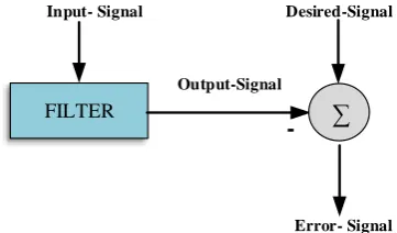
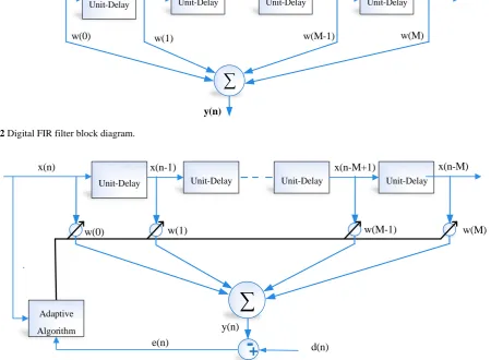
The emphasis of this section is on the general concept of adaptive filtering. Normally, in a filtering problem as shown in Fig. 1, the input signal converts to the desired signal by passing through filter. Achieving this goal requires minimization of the difference between desired signal and filter output (i.e. error function). Fig. 2 illustrates the block diagram of digital FIR filter. As shown in the figure, the filter output (y(n)) is generated as a linear combination of the delayed samples of the input sequence (x(n)) according to:

 

1

  



0

i N

i

y n w x n i







 (1)

where w(i) are FIR filter weights. The set of filter parameters, which optimize this cost function in order to attain maximum adjustment between output and desired signal, should be selected. Adaptive filter is implementation of FIR filter in an intelligent manner [25]. The most commonly used structure for implementation of adaptive filter is the transversal one that is depicted in Fig. 3.

According to Fig. 3, transversal filter has a single

input “x(n)” and an output “y(n)”. The sequence “d(n)”

is the desired signal and e(n) is the prediction error that can be computed from (2). Here “y(n)” is obtained

from (3) where Wi(n)s are time-variant filter weights which adjusted by the adaptive algorithm.

 

e n d n y n (2)

 

1

  



0

N i i

y n w n x n i







 (3)

In summary, adaptive filter refers to any system that takes a mixture of elements from its input and processes them to generate the corresponding set of elements at its output. For attaining this objective, filter coefficient should be updated continuously with the aim of minimizing the cost function. Cost function can be defined as a stochastic, deterministic or transform formulation frame that is briefly reviewed throughout the rest of this section. The performance of the proposed technique has been validated using several real spoof data collections. At first, the spoofing data collection process is described briefly. Then, the performance of suggested algorithms will be analyzed in various schemas.

2.1 Adaptive Algorithms in Stochastic Framework Optimization problem from the stochastic point of view leads to Wiener filter theory. The performance function, which is described for Wiener filer, must be mathematically traceable and should perfectly have only a single minimum. The performance function that meets these requirements is in fact the function of Mean Square Error (MSE) sense that can be written according to:

 

2

ξE e n_ _ (4)

The set of linear equations given by (5) follow from MSE function minimization using direct optimization method which known as Wiener-Hopf equations. Therefore, the set of tap-weight can be obtained analytically by solving them in direct form. In this relation, rxx and rdx are the autocorrelation of x(n) and

cross-correlation between x(n) and d(n), consecutively.

FILTER

Input- Signal

Output-Signal

Desired-Signal

-Error- Signal Fig. 1 The block diagram of filtering problem.

(3)

Unit-Delay Unit-Delay Unit-Delay Unit-Delay

x(n) x(n-1) x(n-M+1) x(n-M)

y(n)

w(0) _w(1) w(M-1) w(M)

Fig. 2 Digital FIR filter block diagram.

x(n) x(n-1) x(n-M+1) x(n-M)

y(n)

w(0) w(1) w(M-1) w(M)

Adaptive

Algorithm

d(n)

-

+

e(n)

Fig. 3 Adaptive transversal filter [22].

It is worth to note that Wiener filters are not FIR filter, they are fundamental to the implementation of adaptive filters.

  



 

1

N

xx dx

l

w l r n l r n





 



(5)

Although direct minimization of (2) to obtain necessary information for design of Wiener filter is possible, due to considerable amount of saving in memory, delay disappearance in the filter output, fast tracking capability of input variation, simplicity in software programming and hardware implementation, an indirect method named steepest-descent (iterative search methods) can be used to achieve this purpose. Obtaining optimum Wiener filter coefficient using steepest-descent method leads to the recursive equation given by:





 

2

1 _k

k

w n w n µ

w n µ E e n



   

 

   _ _ (6)

where μ is a positive scalar called step-size, and ∇kξ

denotes the gradient vector ∇ξ evaluated at the point

w = w(k).

Searching methods to gain optimum Wiener filter coefficients are in fact the adaption algorithms that will be studied in the rest of this section. Access to the minimum of MSE function using direct or indirect manner requires certain statistics such as averaging of whole samples from the beginning until now, which may not be possible in practical applications. For solving this problem, the signal can be assumed ergodic. As a result, instantaneous averaging of error signal can be used instead of ensemble averaging.

In order to achieve this goal for search methods, very rough estimate of the required statistical characteristics is used. The Least Mean Square (LMS) algorithm is utilized for this purpose. According to (7), the instantaneous value of the square of the error signal is used as an estimation of the MSE. Equation (7) after simplification can be reduced to (8), where µ is the algorithm step-size that controls the speed of the convergence.





 

2

1 _k

w n w n  µ E e n_ _ (7)



1



 

2

   

w n w n  µe n x n (8)

(4)

In recent years, for the aim of increasing performance of the conventional LMS algorithm, a number of modifications have been proposed which are described below.

2.1.1 Sign Algorithm

Some adaptive filter applications such as digital signal processing devices, Field-Programmable-Gate-Array (FPGA) targets and application-specific integrated circuits require a simplified version of the standard LMS algorithm.

This algorithm updates the coefficients of an adaptive filter using (9). This equation is obtained from the recursion form of (8) by applying the sign function to the error signal e(n). So, only direction of the gradient is considered. In this recursion, when e(n) is zero, this algorithm does not involve multiplication operations and when e(n) is not zero. This algorithm involves only one multiplication operation. Therefore, implementation of this recursion may be cheaper than the conventional LMS.





 



 



 



 



   

1 sign

/

w n w n e n x n

w n e n e n x n

 

  

  ₍₉₎

2.1.2 Affine Projection Least Mean Square Algorithm (APLMS)

Affine Projection LMS algorithm is obtained by solving the following constraint problem.

Problem: Input matrix and the desired vector of the algorithm consist of the set of tap-input vectors x(n),

x(n-1), …, x(n+1-M) and the set of desired output samples d(n), d(n-1), …, d(n+1-M), consecutively. Choose the updated tap-weight vector w(n+1) in a way that minimizes the squared Euclidian norm of the difference which is described in (10), subject to the set of constraint (11):

( ) ( 1) - ( )

N n W n W n (10)



1

 







T

W n x nk d nk (11)

Solving this problem using the method of Lagrange multiplier results in adaption (12):





 

   

1

   

1

T

w n w n

µ X n X n I  X n e n

 

 

 _  _ ₍₁₂₎

where µ and ψ are constant parameters that control the convergence speed and stability of the algorithm. APLMS algorithm offers a significant convergence improves as M increases. This improvement comes at the cost of additional computational complexity, as can be seen in (12). Here, in contrast with conventional LMS algorithm, in which the step-size is constant and

there is a probability of passing the global minimum, the

step-size is equal to µ X_ T

   

n X n I_1 which varies with time (proportional to the power spectral density of input signal) and contributes to higher accuracy.

2.1.3 Normalized Least Mean Square

For M = 1, APLMS algorithm is reduced to Normalized LMS (NLMS) algorithm. In this sort of algorithm, the step-size parameter for every recursion will normalize proportional to the power of the input signal. Thus, the recursive equation for tap-weight adjustment with considering two degrees of freedom for step-size parameter can be derived according to (13). In this equation, α and β are positive constants which control the step-size of the algorithm and

 

2

x n is the power of the input signal.





 



 

2



   

1 /

W n w n  x n  e n x n (13)

2.1.4 Variable Step-Size Least Mean Square Algorithm

Until now, some types of modified LMS algorithms are studied. The step-size parameter plays a vital role in controlling performance of the LMS algorithm. In fact, a large step-size parameter may be required to minimize the transient time of the LMS algorithm. On the other hand, to obtain a small miss-adjustment, a small step-size parameter has to be used. Consequently, the existence of a significant algorithm, which can establish a tradeoff between these two conflicting requirements, is necessary. In other words, an algorithm is required which can consider adaptive changes for the step-size parameter. The Variable Step-size LMS (VSLMS) algorithm is one of the most effective solutions for this problem. The operation of such an adaptation is as follows. Each tap of the adaptive filter has a separate time-varying step-size parameter and the LMS recursion is according to (14), where wi(n) is the i-th element of

the tap-weight vector w(n) and μi(n) is its associated

step-size parameter at iteration n. It is noteworthy that in all other algorithms which have been studied up to now, weights have the same step-size.



1



 

    



i i i

w n w n µ n e n x ni (14)

The corresponding gradient term that should move opposite of its direction for each element of weight vector is obtained from (15):

    



i

g n e n x ni (15)

where μi(n) have to be increased if the gradient term

consistently shows positive or negative direction. This happens when the adaptive filter has not yet converged.

(5)

As the adaptive filter tap weights converge to some vicinity of their optimum values, the average of the gradient terms approaches to zero and hence its sign changes more frequently. In other words, it fluctuates around zero. In this condition, the corresponding step-size parameters are gradually declined to some minimum values until optimum points be recognized. Following the above argument, the VSLMS algorithm step-size parameters, μi(n), may be adjusted using the

recursive equation as:

 





 





1

sign sign 1

i i

µ n µ n

g n g n



 

 _ _ _  _ (16)

2.2 Adaptive Algorithm in Deterministic Framework In addition to adaptive filtering algorithms which have origin in a statistical formulation of the problem, there exists a second category of algorithms that in this case the adaptive filter coefficients are adjusted with minimizing deterministic function (sum weighted square error), as can be seen in (17), where ρn(k) is a

weighting function [24]. This method is named least square.

 

   

2

1

n

n n

k

n k e k

 





(17)

Here similar to statistical optimization, direct method of minimization is not suitable for practical implementation of adaptive filters. As a result, recursive method is utilized to minimize (17) by Recursive-Least-Squares (RLS) algorithm. In RLS algorithm, weight function for estimation error is obtained from (18):

 

n k , 1, 2, ,

n k k n

 _  _

(18)

where, λ is a positive constant that is known as forgetting factor. By putting the cost function gradient equal to zero, recursive (19) for weight vector adaption will be obtained, where eˆn1

 

n and k(n) are computed

according to (20) and (21). In (19), k(n) is gain vector and ψ(n) follows from recursive (22).

 



1



 

ˆ 1

 

ˆT ˆT

n

w n w n k n e  n (19)

 



  

1

ˆ ˆT 1

n

e  n d n w n x n (20)

 



  

 



  

1 1

1

1 T 1

n x n

k n

x n n x n



  

 

 

 

  (21)

 

n



n 1



X n X

 

T

 

n

 

    (22)

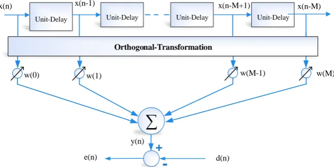
2.3 Adaptive Algorithm in Transform Framework (TDAF)

It is known that convergence behavior of LMS algorithm is highly dependent on eigen values of the input correlation matrix that is related to power spectral density of input sequence and so is frequency dependent. Subsequently, optimum filter tap-weight (wo(ejω)) can be determined in a transformed (such as

frequency) domain. The rate of convergence of w(ejω) toward its optimum value at a given frequency ω = ωo,

is in direct relation with the value of the power spectral density of the input signal at ω = ωo. It is worth to note

that TDAF compared to time domain LMS has faster convergence speed and efficient implementation. The block diagram of transform domain adaptive filtering is depicted in Fig. 4. As illustrated in this figure, an orthogonal transformation (xT(n)=T{x(n)}) is

applied to input sequence before the filtering process. Where ‘x(n)’ and ‘xT(n)’ are filter input string in time

and transform domain consecutively, and ‘T’ is

transformation matrix (should be unitary matrix). Orthogonal property of transformation matrix is shown in (23):

1

T T

T T TT  (23)

Thus, filter tap-weights vector (wT(n)) are optimized in

transformed domain, with the goal of MSE minimization. The FIR filter output and error function are obtained from (24) and (25), respectively, in time

x(n) x(n-1) x(n-M+1) x(n-M)

y(n)

w(0) w(1) w(M-1) w(M)

d(n)

-+

e(n)

Orthogonal-Transformation

Fig. 4 The block diagram of transform domain adaptive filtering.

(6)

domain (y(n) and e(n) are still in time domain).

 

T

   

T T

y n w n x n (24)

 

e n d n y n (25)

Furthermore, by calculating the inverse transform of “wT(n)”, y(n) can be obtained from:

 

T

   

y n w n x n (26)

The cost function utilized to optimize the filter weights, is “ξ =E[e2₍_n_{)]”. By using (24) and (25), this function} can be expressed as:

 

2

T T

T T T T T

w R w w p E d n

  _{ } _ (27)

where RT = E[xT(n) xTT(n)] and PT = E[d(n) xT(n)].

Therefore, optimum tap-weight vector can be gained according to (28) and so the minimum value of MSE is obtained from (29) that is equal to the minimum value of cost function that calculates for time domain adaptive filter in [24].

1 ,

T O T T

w R P (28)

 

2 1

min

T

E d n p R p

 _ _ __ 

  (29)

2.3.1 Transform Domain LMS algorithm

Adjustment recursion for filter tap-weight of TDLMS algorithm is expressed as:





 

1

   

1 2 ˆ

T T T

w n w n  D e n x n (30)

where ˆD is a diagonal matrix (it’s elementsare the power spectral density of input elements). The vector (30) can be expressed as N scalar recursions for each tap-weight of the filter according to:





 

   

 

,

, 1 , 2 _ˆ2 ,

T i

T i T i T i

x

w n w n e n x n

n

 

   ₍₃₁₎

where ˆ

 

T,i

2 x

σ n is an estimate of E[xT₍_n₎_x

TT(n)] that can

be calculated from recursion (32) for each tap-weights of this filter.

 

ˆ



 

  

T,i T,i

2 2

x x T,i

σ n = βσ n -1 + 1- β x n (32)

where, β is a positive constant close to but less than one. The three main type of TDLMS algorithms in discrete domain that have been used in this paper are CDTLMS, FFTLMS and DWTLMS algorithms. These robust algorithms, as mentioned before, containing three significant steps: transformation (discrete cosine, fast furrier and discrete wavelet transform), power normalization and LMS adaptive filtering. They work almost as well as RLS algorithm, but may outweight RLS algorithm from stability and robustness perspective.

3 Adaptive Filtering Approach for GPS Interference Cancelation

When the received GPS signal in the target receiver is a mixture of the desired signal and interference, which can be produced by intentional or unintentional sources, an adaptive filter under certain circumstances can be designed to reduce interference [25]. The principle of using adaptive filters to eliminate interference is to obtain an estimate of interfering signal and subtract that from the corrupted signal. Therefore, what remains at the output is the desired signal. This method can be feasible if the interfering signal source is accessible. It will be note later that this condition is not practical. However, our proposed algorithm have a proper solution to solve this problem. Fig. 5 depicts the concept of using an adaptive filter to reduce interference. It is worth to note that the objective of the approach presented in this section is the filter tuning for further operation.

As is evident, the filter has two inputs. Actually from Fig. 3 the x(n) and d(n). x(n) and d(n) are utilized as reference and primary inputs, respectively. According to (33) the primary input“d(n)” is the corrupted signal

that is the mixture of authentic GPS signal “s(n)” and

interference component “x'(n)”. Moreover, the reference

input “x(n)” was generated from the interference source

only. In summary, for interference cancelation, interference in reference signal is the filter input and the interference component of primary input is authentic GPS signal that the adaptive filter tries to establish a replica of this at its FIR filter output “y(n)”. For this

reason, interference that originates from interference source is named reference input.

 

d n s n x n (33)

Desired Signal

Interference Signal

Adaptive FIR Filter Primary Input

Reference Input

e(n) d(n)

x(n)

+

_

y(n)

Fig. 5 Using adaptive filter for interference cancelation [25].

(7)

In order to achieve interference free signal at the adaptive filter output, as mentioned in the following conditions, the authentic GPS signal should be uncorrelated with interference component in both primary and reference inputs and the reference signal should be correlated with the interference component of primary input.

(a) E s n x n - k = 0 , n,k = 0,1,2,…,n -1_

  





_ .

(b) E s n x n - k = 0 , n,k = 0,1,2,…,n -1_

  



_ .

(c)

  



 

.

 

 

E x n x n - k = p k , n,k = 0,1, 2,…

, n - 1

In recent relation, “p(k)” is an unknown cross-correlation between reference input and the authentic GPS signal. Based on recent signal modeling, estimation error is obtained as:

 

     

   

e n = d n - y n = s n + x' n - y n (34)

According of standard model, “d(n)” will be equals to

“y(n)” approximately after converge of the algorithm and “e(n)” is error of estimation. State is kindly

different here. “d(n)” is sum of authentic and interference GPS signal and “y(n)” is estimate of

authentic signal. It is obvious that these are not equal. However, the algorithm tries to minimize this phrase. As explained later during minimizing process “y(n)”

nullifies the “x'(n)” component of primary signal and

nearly acceptable approximation of authentic GPS signal is yielded at output of the filter as “e(n)” signal.

According to first and second conditions, authentic signal component of primary input “s(n)” is

uncorrelated with reference signal “x(n)”. Thus, “s(n)”

is not be affected by the filter. Therefore, minimization of “e(n)” leads to minimization of “x'(n)-y(n)” and y(n) will be approximately equal x'(n) to [25]. By subtracting “y(n)” from “d(n)”, authentic signal

component would appear in the output of the overall adaptive filter.

As mentionedjust above, existence of only one copy of delayed signal at the reference input is crucial to achieve “x'(n)” at the output of FIR filter. However, in

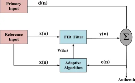
actual processing, this is not accessible. So, modeling of the system must be changed. Since the mixture of both delay and original signal at the input is available. Bearing in mind that in here, two delays spoof signal are used as primary and reference inputs. As shown if Fig. 6 each one of which can be modeled as:

   

delay

 

d n = s n + x n (35)

 



 

_delay

 

x n = s n + x n (36)

In the modified signaling model for real condition, “xdelay” and “x’delay” are delayed components in primary and reference inputs, respectively. “s(n)” and “s’(n)” are

authentic GPS signals of primary and reference inputs. The previous studies was done in 1997 by Han and Rizos, indicate that “s(n)” and “s’(n)” are uncorrelated.

On the other hand, “xdelay” and “x’delay” have correlation with each other [25]. Also, in the presented paper by the aforementioned authors, this matter has been proved on multi-path. Because of multi-path and delay spoofing similarity, this theorem can also be generalized to spoofing.

With passing primary and reference input through the adaptive filtering system, the FIR filter estimates the component of primary input that is correlated with a component of reference input. Consequently, as illustrated in Fig. 6 the correlated component is the direct output of the FIR filter and the uncorrelated component is the output of the whole adaptive filtering system. The conducted simulations indicate that the adaptive filter enables distinguishing the delayed component of spoof signal and removes it from primary signal. It is worth to note that Fig. 5 is model of filtering problem in ideal condition and Fig. 6 is its modified version of Fig. 5 for explained real condition.

4 Test Results

The performance of the proposed techniques has been validated using several real spoof data collection and simulated replay spoofing scenario. At first, the spoofing data collection process is described briefly. Then, the performance of suggested algorithms will be analyzed in various schemas.

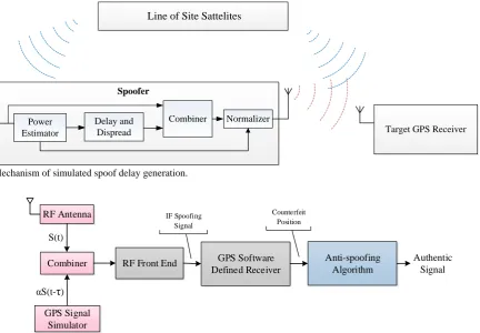
4.1 Mechanism of Spoof Delay Generation

Spoofer transmits the fake signal to target receiver in either synchronous or asynchronous manner. In the case of synchronous attack, spoofing signal with aligned correlation peak will be generated.

In asynchronous attack, a GPS signal simulator transmits higher power forgery correlation peak that is not aligned with authentic peak towards the target receiver. A synchronous attack is still difficult to implement and asynchronous attack is a more realistic scenario [10,11].

Primary Input

Reference

Input FIRFilter

Adaptive Algorithm

Σ

x(n) x(n) d(n)

Wi(n)

y(n)

Authentic Signal

e(n)

Fig. 6 Spoof reduction by the adaptive filter.

(8)

Delay spoof is an asynchronous type spoofing that mechanism of its generation for two types of simulated and measured data consecutively are shown in Figs. (7) and (8). As shown in Fig. 7, in the case of simulated delay spoof generation, the input signal is delayed as a proper time and after amplification combined by the authentic signal at IF level. GPS signal generated by the spoofer is propagated toward target receiver (with certain delay) concurrent with next signals. For generating measured delay spoof, the RF signals from a simulator were combined instead of IF to deliverance from quantization error due to the A/D in the front-end module (Fig. 8). The corrupted signal in this case can be expressed in (37):

 

ˆ





d n S n S n (37)

where “α” is amplification, factor which is equal to 2 here. According to the mentioned modeling in section 3, “S nˆ







” is actually considered as interference

element “xdelay”. Moreover, “S nˆ

 

” likely is the GPS authentic signal. In this scenario, it is generally assumed that simulator’s output S nˆ

 

is much the same signal directly taken from the GPS antenna. After the RF input signal is converted into a digital IF signal and before satellite acquisition, spoofing attack applies to the data.

4.2 Test Results of Mitigation Algorithm

The spoof reduction results using adaptive filtering technique for both measured and simulated static data are compared in Table 1. Real GPS receiver collects the base signal of both simulated and measured spoof data. The counterfeit signal of simulated spoofing is generated in software, but GPS signal generator is utilized for measured spoofing data. Moreover, combination of IF signals for simulated data is done in software. RF signals of measured data are combined in real combiner. Simulated spoofing data set contains more than 1000 sample.

The most significant feature based on the presented information is that spoof reduction result for most of the cases is well over 70 percent. «spoof reduction» is the ratio between RMS position errors with and without the filter. The stronger signal is the spoofing because its source is near to the receiver.

Since the computations are performed on pseudo-range, operation speed is high and time complexity is less than 10 milliseconds in worst case. In the first place, about stochastic framework that contains methods such as conventional LMS, NLMS, APLMS, VSLMS and sign algorithms, the most accurate method is relevant to VSLMS approach that reduced the estimation error to 89 and 81 percent for measurement and simulated data, respectively. In the second place, RLS method as a deterministic framework is able to

Target GPS Receiver

Line of Site Sattelites

Power Estimator

Delay and Dispread

Combiner Normalizer

Spoofer

Fig. 7 Mechanism of simulated spoof delay generation.

RF Antenna

GPS Signal Simulator

Combiner RF Front End S(t)

αS(t-τ)

GPS Software Defined Receiver

Anti-spoofing Algorithm

Authentic Signal IF Spoofing

Signal

Counterfeit Position

Fig. 8 Block diagram of measured spoof delay generator.

(9)

reduce distance error around 85 percent and finally in the case of transformed framework which containing CDTLMS, FFTLMS and DWTLMS algorithm has the best operation in spoof reduction.

A comparison between all algorithms from practical point of view is summarized in Table 2. It is worth to note that positioning accuracy; real errors during the spoofing before and after its reduction are computed based on extracted coordinated by software GPS receiver.

According to the presented data in the Tables 1 and 2, since the step-size of the LMS algorithm in all iterations remains constant, the LMS algorithm has a lower spoof reduction ability than other algorithms. Therefore, it cannot accurately find the global minimum, but the convergence speed of the algorithm was higher than other described algorithms. The sign algorithm has variable step-size, so that when the algorithm comes close to convergence, the step-size will be small and smaller to find a global minimum with a higher accuracy. Thus, in comparison with the LMS algorithm, this one can offer a better tradeoff between accuracy and speed.

Also for APLMS and NLMS algorithms, the step-size is variable and is proportional to the input signal power. These algorithms have lower convergence speed, higher computational complexity and so are more accurate than the conventional LMS algorithm.VSLMS algorithms have higher accuracy than any of the discussed algorithms. The reason is that each tap of the adaptive filter has a separate time-varying step-size parameter which become small and smaller by approaching to convergence [25]. Hence, for the case of

VSLMS algorithm, the number of iterations is higher than other algorithms.

In deterministic framework, the RLS algorithm like modified LMS algorithms, is variable step-size approach that this feature has greatly enhanced the accuracy and this increased accuracy leads to speed reduction. Finally, in TDAF algorithms step-size also governs the convergence speed and steady state miss-adjustment. Besides, selected unitary transformation matrix strongly influences the filter performance, especially when the filter length is short. Here, for the purpose of GPS signal spoof reduction and with respect to order of designed filter, DCT, FFT and DWT (Haar) had a better performance compared to other unitary transformations.

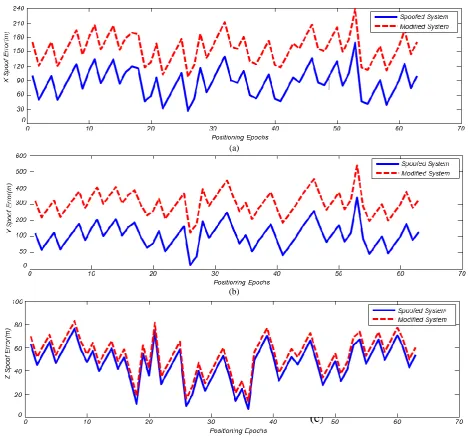
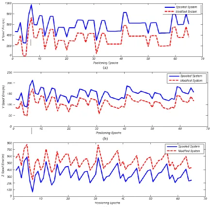
After conducting various tests considering the above-mentioned notes, the VSLMS algorithm has the best performance. This algorithm, as the most accurate case applied to measurement spoof GPS data set that has 4, 6 and 8 seconds delay and so caused 157, 263 and 455 meters error in positioning solution, consecutively. Results are depicted in Figs. (9) to (11).

As indicated in figures, this filter mitigated delay spoof from spoof data in all three dimensions. Modified system is the GPS receiver equipped with anti-spoofing algorithm. Real GPS receivers performs smoothing algorithm to decrease scattering of positioning which is not exist in the investigated software GPS receiver. To be more precise, according to two-line graph in Fig. 9, for 4 seconds delayed spoof signal, designed VSLMS algorithm is able to reduce distance error around 140, 68 and 21 meter in x, y and direction

Table 1 Results of measurement spoof reduction percentage.

Spoof reduction (%) Framework

Algorithm

Simulated data Measurement data

73 72

Stochastic LMS

76 88

NLMS

77 78

APLMS

81 89

VSLMS

78 88

Sign

76 85

Deterministic RLS

75 81

Transform CDTLMS

69 72

FFTLMS

76 83

DWTLMS

Table 2 Comparison between mentioned algorithms.

Algorithm Hardware complexity Convergence speed Accuracy Usability in real-time applications

LMS Low High Middle Yes

Sign Low Middle High Yes

NLMS Middle Middle High Yes

APLMS High Middle High Yes

VSLMS Middle Low High Yes

RLS Middle Middle High Yes

CDTLMS Middle High High Yes

FFTLMS Middle High Middle Yes

DWTLMS Middle High High Yes

(10)

Iranian Journal of Electrical & Electronic Engineering, Vol. 14, No. 3, September 2018 231 (a)

(b)

(c)

Fig. 9 Variation of pseudo-range for interferential GPS data (157 meters error) before and after filtering using the VSLMS algorithm: a) x-component, b) y-component and c) z-component.

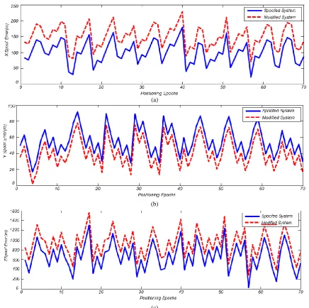
consecutively. In the case of 6 seconds delayed spoof signal, mentioned algorithm declined distance error by 185, 169 and 79 meter in x, y and z direction, respectively. Finally, about 8 seconds spoof delayed signal, discussed algorithm is able to eliminated distance error about 380, 328 and 270 meter in x, y and z

directions, respectively. It is obvious that the most error mitigation is along x axis and this fact results from the nature of spoof signal.

The average values of spoof mitigation by VSLMS algorithm are listed in Table 3, which mitigates interference within an average of 89% and a tolerance of 16%. The “mitigation average” indicates mean of reduction percentages. The difference between the highest and the lowest reduction percentage reported as “Tolerance”. A comparison between the proposed method and other interference reduction methods in

pseudo-range level has been listed in Table 4. As mentioned in table, the RAIM method increases complexity of algorithm and it is inefficient in the presence of multi-path.

Neural network estimator is easy to implement, but error increases in long time spoofing. Adaptive filtering technique is easy to implement, yet it is an accurate method in comparison with other techniques in navigation level.

Table 4 presents properties discussed in Section 1 and suggested algorithm on the examined factors, required equipment, limitations and advantage of approaches. In order to have a better judgment, a numerical value was assigned to each feature. The worst and the best cases are considered for any feature; score 0 is dedicated for the worst state and 10 score is devoted for the best state. After that, a number ranged 0 to 10 is assigned to any

(11)

(b)

(c)

Table 3 Result of spoof reduction in RMS from measured spoof data using VSLMS algorithm.

Spoof reduction (%) 3D positioning error after filtering (m)

3D positioning error before filtering (m) Spoof data’s delay (sec)

96 6

157 4

80 53

263 6

91 40

455 8

Table 4 Comparison between the suggested method and other interference reduction techniques.

Total mark Limitations

Advantages Required equipment

Analyzed features Detection

methods

18 Inefficient in synchronous attacks, need prior data (2) Easy detection (5)

Software upgrade (6) Correlation branch (5)

SQM

19 Inefficient in synchronous attacks, need prior data (5) Ability to multipath

separation (7) Software and hardware upgrade (3)

Correlation branch (4) VSD

16 High cost and complexity (3) High recognition

accuracy (8) Additional tracking loop (2)

Correlation branch (3) VB

16 Unreliable in more than two

counterfeit satellites (2) Easy to implement (5)

Software upgrade (6) Pseudo-range (3)

RAIM

21 Algorithm needs prior data (5) High accuracy (7)

Software upgrade (6) Navigation (3)

This work

(12)

(b)

(c)

feature depending on the algorithm performance. For example, about the feature “necessary equipment”, an algorithm takes 10 if no extra equipment is needed. Besides, in case of necessity to basal changes in receiver structure, it earns 0 [2]. As can be seen, the proposed algorithm performs better than the other ones on account of the fact that offered method needs no extra hardware and does not increase the receiver size and the production costs.

5 Conclusion

Adaptive filter is a powerful signal analyzer that can estimate interference component of the delay spoof signal at the output of the filter core by adjusting its weights that conducting using adaptive algorithms. In this paper, adaptive algorithm in three types of statistical (LMS algorithm and its modified types),

deterministic (RLS algorithm) and transform frame were studied. The results show that all investigated algorithms decrease positioning error up to 70 percent and VSLMS as most intelligent algorithm that established better tradeoff between accuracy and speed in comparison with other variable step-size approach. VSLMS algorithm has the best performance for interference cancelation and decreases spoof delay error to 89 percent.

References

[1] T. Nighswander, B. Ledvina, J. Diamond, R. Brumley and D. Brumley, “GPS Software Attacks,” International Conference on Computer Communication Networks-Security and Protection, pp. 450–461, 2012.

(13)

[2] M. Moazedi, M. R. Mosavi and A. Sadr, “Real-Time Interference Detection in Tracking Loop of GPS Receiver,” Iranian Journal of Electrical and Electronic Engineering, Vol.13, No.2, pp. 194–204, 2017.

[3] M. R. Mosavi, A. R. Baziar and M. Moazedi, “De-noising and Spoofing Extraction from Position Solution using Wavelet Transform on Stationary Single-Frequency GPS Receiver in Immediate Detection Condition,” Journal of Applied Research and Technology, Vol. 15, No. 4, pp. 402–411, 2017. [4] T. Kim, S. Cheon and L. Sanguk, “Analysis of

Effect of Spoofing Signal in GPS Receiver,”

International Conference on Control, Automation and Systems, pp. 2083–2087, 2012.

[5] T. E. Humphreys, J. Bhatti, D. Shepard and K. Wesson, “The Texas Spoofing Test Battery: Toward a Standard for Evaluating GPS Signal Authentication Techniques,” 25th_{International}

Technical Meeting of the Satellite Division of the Institute of Navigation, pp. 3569–3583, 2012. [6] A. Javaid, F. Jahan and W. Sun, “Analysis of

Global Positioning System-based Attacks and a Novel Global Positioning System Spoofing Detection/Mitigation Algorithm for Unmanned Aerial Vehicle Simulation,” Simulation: Transactions of the Society for Modeling and Simulation International, Vol. 93, No. 5, pp. 427– 441, 2017.

[7] A. Broumandan, A. Jafarnia and G. Lachapelle, “Spoofing Detection, Classification and Cancellation Receiver Architecture for a Moving GNSS Receiver,” Journal of GPS Solutions, Vol. 19, No. 3, pp. 475–487, 2015.

[8] M. R. Mosavi, A. Nakhaei and S. Bagherinia, “Improvement in Differential GPS Accuracy using Kalman Filter,” Journal of Aerospace Science and Technology, Vol. 7, No. 2, pp. 69–80, 2010.

[9] M. R. Mosavi, “Comparing DGPS Corrections Prediction using Neural Network, Fuzzy Neural Network, and Kalman Filter,” Journal of GPS Solutions, Vol. 10, No. 2, pp. 97–107, 2006.

[10]L. Bao, R. Wu, W. Wang and D. Lu, “Spoofing Mitigation in Global Positioning System Based on C/A Code Self-coherence with Array Signal Processing,” Journal of Communications Technology and Electronics, Vol. 62, No. 1, pp. 66– 73, 2017.

[11]S. Krasovski, M. Petovello and G. Lachapelle, “Ultra-tight GPS/INS Receiver Performance in the Presence of Jamming Signals,” International Technical Meeting of the Institute of Navigation, pp. 1–13, 2014.

[12]A. J. Jahromi, T. Lin, A. Broumandan, J. Nielsen and G. Lachapelle, “Detection and Mitigation of Spoofing Attacks on a Vector-based Tracking GPS Receiver,” International Technical Meeting of the Institute of Navigation, pp. 3–8, 2012.

[13]A. J. Jahromi, J. Broumandan, A. Nielsen and G. Lachapelle, “GPS Vulnerability to Spoofing Threats and a Review of Anti-spoofing Technique,”

International Journal of Navigation and Observation, pp. 1–16, 2012.

[14]N. A. White, P. S. Maybeck and S. L. Devilbiss, “Detection Interference, Jamming and Spoofing in a DGPS-Aided Inertial System,” IEEE Transactions on Aerospace and Electronic Systems, Vol. 34, No. 4, pp. 1208–1217, 1998.

[15]S. Amiri, M. A. Dalir and H. Talaiee, “GPS Signal Simulation in Intermediate Frequency (IF),” Journal of Space Science and Technology, Vol. 5, No. 3, pp. 33–40, 2012.

[16]B. M. Ledvina, W. J. Bencze, B. Galusha and I. Miller, “An In-Line Anti-Spoofing Device for Legacy Civil GPS Receivers,” The 23rd

International Technical Meeting of the Institute of Navigation, pp. 689–712, 2010.

[17]A. Cavaleri, B. Motella, M. Pini and M. Fantino, “Detection of Spoofed GPS Signals at Code and Carrier Tracking Level,” Satellite Navigation Technologies and European Workshop on GNSS Signals and Signal Processing, pp. 1–6, 2010. [18]K. D. Wesson, D. P. Shepard, J. A. Bhatti and

T. E. Humphreys, “An Evaluation of the Vestigial Signal Defense for Civil GPS Anti-Spoofing,” The 24th_{International Technical Meeting of the Satellite}

Division of the Institute of Navigation, pp. 1–11, 2011.

[19]M. Lashley and D. Bevly, “What About Vector Tracking Loops?,” Inside GNSS Magazine, pp. 1–6. 2009.

[20]Z. Zhenghao, M. Trinkle, Q. Lijun and L. Husheng, “Quickest Detection of GPS Spoofing Attack,”

Military Communications Conference, pp. 1–6. 2012.

[21]M. Berardo, E. Garbin, M. Fabio, D. Letiziab and L. Presti, “A Spooﬁng Mitigation Technique for Dynamic Applications,” Satellite Navigation Technologies and European Workshop on GNSS Signals and Signal Processing, pp. 1–7, 2016. [22]H. Li and H. Dai, “Quickest Spectrum Sensing in

Cognitive Radio,” International Conference on Information Sciences and Systems, pp. 203–208, 2008.

(14)

[23]A. Farhadi, M. Moazedi, M. R. Mosavi and A. Sadr, “A Novel Ratio-Phase Metric of Signal Quality Monitoring for Real-Time Detection of GPS Interference,” Journal of Wireless Personal Communications, Vol. 97, No. 2, pp. 2799–2818, 2017.

[24]B. F. Boroujeny, Adaptive Filters Theory and Applications. John Wiley & Sons., Second Edition, 2013.

[25]L. Ge, S. Han and C. Rizos, “Multipath Mitigation of Continuous GPS Measurements using an Adaptive Filter,” Journal of GPS Solution, Vol. 4, pp. 19–30, 2000.

[26]N. Carson, S. M. Martin, J. Starling and D. M. Bevly, “GPS Spoofing Detection and Mitigation using Cooperative Adaptive Cruise Control System,” IEEE Intelligent Vehicles Symposium, pp. 19–22, 2016.

P. Teymoori received her B.Sc. degree in Electronic Engineering from respectively Shahid Beheshti University (SBU) in 2012. She is a M.Sc. student in Iran University of Science and Technology (IUST), Tehran, Iran. Her current research interests include GPS signal processing and filtering.

M. R. Mosavi received his B.Sc., M.Sc., and Ph.D. degrees in Electronic Engineering from Iran University of Science and Technology (IUST), Tehran, Iran in 1997, 1998, and 2004, respectively. He is currently faculty member (Full Professor) of the Department of Electrical Engineering of IUST. He is the author of more than 330 scientific publications in journals and international conferences. His research interests include circuits and systems design.

M. Moazedi received her B.Sc., M.Sc. and Ph.D. degrees in Electronic Engineering from Iran University of Science and Technology (IUST), Tehran, Iran in 2008, 2011 and 2018, respectively. Her research interests in the area of analog and mixed signal integrated circuits.

access article distributed under the terms and conditions of the Creative

Commons Attribution-NonCommercial 4.0 International (CC BY-NC 4.0)

license (https://creativecommons.org/licenses/by-nc/4.0/).

Downloaded from ijeee.iust.ac.ir at 14:48 IRDT on Friday September 18th 2020 [ DOI: 10.22068/IJEEE.14.3.222 ]