Journal of Chemical and Pharmaceutical Research, 2016, 8(5):889-894
Research Article
CODEN(USA) : JCPRC5
ISSN : 0975-7384
Improved Adaptive Time Delay Estimation Algorithm Based on
Fourth-order Cumulants
Ling Tang and Yumei Chen
College of Automation and Electronic Information, Sichuan University of Science & Engineering, Zigong 643000, China
_____________________________________________________________________________________________
ABSTRACT
Time-delay estimation is widely used in sonar and radar applications. In order to estimate time delay accurately in variable signal to noise ratio(SNR), an improved algorithm of adaptive time delay estimation(TDE) based on fourth-order cumulants has been proposed in this paper. The single adaptive filter in the conventional model is separated into two adaptive subunits connected in cascade, one is to track the delay, the other to track the SNR, so as to obtain the accurate signal time delay estimation in the low and variable SNR. The theoretical analysis and simulation results confirm the validity and feasibility of the proposed algorithm.
Keywords: fourth-order cumulants, time delay, adaptive filter, variable SNR
_____________________________________________________________________________________________
INTRODUCTION
Time Delay Estimation(TDE) as an active research in signal processing is widely used in the fields of radar, sonar, communication and so on. The common methods are phase method, double spectrum method, correlation method, adaptive filter parameter model method and so on. With the continuous development of signal processing methods, a variety of algorithms are introduced into time delay estimation, which improves the precision and convergence, reduces the computation. Because of blind Gauss property high order accumulation is widely used in time delay estimation. Liu Ying et al.[1] proposed an adaptive time delay estimation algorithm based on four-order cumulants(FOC-LMSTDE), which can effectively suppress the influence of correlated Gauss noise, but in the case of low SNR the estimated results are not satisfactory. Aiming at this problem, a new algorithm of time delay estimation algorithm FOC-ETDE is proposed in the literature[2], which can suppress the impact of related or not related to Gauss noise, and obtain the accurate time delay estimation of non Gauss signal in lower SNR. However when SNR changes, the performance of the system is greatly reduced.
In this paper, an improved adaptive time delay estimation algorithm is proposed. The single adaptive filter is separated into two adaptive subunits connected in cascade, one is to track the delay, the other to track the SNR, so as to improve the performance in the variable SNR.
MATHEMATICAL MODEL
Consider one signal beamed from a distant source, with interference and noise in the channel. Thus the signal parameter model received on two spatially separated sensors[3] is:
)
(
)
(
)
(
k
s
k
w
1k
x
=
+
(1))
(
)
(
)
(
k
as
k
D
w
2k
In the formula
s
(k
)
is non Gauss and zero mean stationary random signal,s
(
k
−
D
)
is the time delay of)
(k
s
,a
is the fading factor that satisfieda
∈
(
0
,
1
]
, usuallya
=
1
.w
1(
k
)
andw
2(
k
)
are the correlative zero mean Gauss noises which is independent withs
(k
)
.By convolution theory:
∑
∞ −∞ =−
−
=
−
n
n
k
s
D
n
c
D
k
s
(
)
sin
(
)
(
)
(3)Where
v
v
v
c
(
)
sin(
π
)
π
sin
=
, then replace∞
with a large positive integerp
(p
>
D
), and ignoring the truncation error, we can get the sampling values of the function.Insert the formula (3) into (2):
∑
− =+
−
−
=
pp i
k
n
i
k
s
D
i
c
a
k
y
(
)
sin
(
)
(
)
2(
)
=a
sin
c
(
i
D
)
[
x
(
k
i
)
n
1(
k
i
)
]
n
2(
k
)
p
p i
+
−
−
−
−
∑
− =(4)
The purpose of time delay estimation is to suppress the Gauss noise effectively by using the limited observation signal
x
(
k
)
andy
(
k
)
, so as to estimate the time delayD
.ALGORITHM ANALYSIS
For stationary random process with zero mean
x
(
k
)
andy
(
k
)
, the FOC of the random variablex
(
k
)
can be defined as follows:)]
(
),
(
),
(
),
(
[
)
0
,
0
,
(
cum
x
k
x
k
x
k
x
k
C
xxxxτ
=
+
τ
(5)Define cross four order cumulants(CFOC) of the random variables
x
(
k
)
andy
(
k
)
as:)]
(
),
(
),
(
),
(
[
)
0
,
0
,
(
cum
x
k
y
k
x
k
x
k
C
xyxxτ
=
+
τ
(6)Insert the formula (4) into (6), we get
1 2
( ,0,0)
( ),
sin (
)[ (
)
(
)]
(
), ( ), ( )
p
xyxx
i p
C
τ
cum x k a
c i
D x k
i
τ
w k
i
τ
w k
τ
x k x k
=−
=
−
− + −
− +
+
+
∑
(7)According to the properties that the cumulants can be added and the FOC of Gauss noise is zero, the equation(7) can be sorted out:
[
(
),
(
),
(
),
(
)
]
)
(
sin
)
0
,
0
,
(
a
c
i
D
cum
x
k
x
k
i
x
k
x
k
C
p
p i
xyxx
τ
=
∑
−
−
+
τ
− =
(8)
That is:
)
0
,
0
,
(
)
0
,
0
,
(
τ
ssssτ
xxxx
C
C
=
(9)∑
∑
− = −
=
−
−
=
−
−
=
pp i
ssss p
p i
xxxx
xyxx
a
c
i
D
C
i
a
c
i
D
C
i
C
(
τ
,
0
,
0
)
sin
(
)
(
τ
,
0
,
0
)
sin
(
)
(
τ
,
0
,
0
)
(10)Apparently the Gauss noise contained in
C
xxxx(
τ
,
0
,
0
),
C
xyxx(
τ
,
0
,
0
)
is suppressed. The formula (10) can be expressed as a vector:S
aC
______________________________________________________________________________
Where,a
is the constant, andT
D
p
c
D
p
c
D
p
c
S
=
[sin
(
−
−
),
sin
(
−
+
1
−
),
L
,
sin
(
−
)]
[
]
Txyxx xyxx
xyxx
xy
C
p
C
p
C
p
C
=
(
−
,
0
,
0
),
(
−
+
1
,
0
,
0
),
L
,
(
,
0
,
0
)
−
+
−
−
−
=
)
0
,
0
,
0
(
)
0
,
0
,
1
2
(
)
0
,
0
,
2
(
)
0
,
0
,
1
2
(
)
0
,
0
,
0
(
)
0
,
0
,
1
(
)
0
,
0
,
2
(
)
0
,
0
,
1
(
)
0
,
0
,
0
(
4 xxxx xxxx xxxx xxxx xxxx xxxx xxxx xxxx xxxx xC
p
C
p
C
p
C
C
C
p
C
C
C
C
L
M
O
M
M
L
L
In the use of adaptive time delay estimation method to get the time delay, the optimal weight coefficient should be [4]: T w s s
p
p
p
p
i
D
i
c
a
]
,
1
,
,
0
,
,
1
,
),
(
[sin
2 2 2−
+
−
−
=
−
+
⋅
L
L
σ
σ
σ
(12)Based on the maximum value of the weight coefficient, TDE is obtained. However this method can get the maximum error in the case of low noise, which leads to inaccurate estimation. In this case, the original adaptive filter coefficients can be decoupled into two parts of
g
andsin
c
, with usingsin
c
(
i
−
D
)
filter, at the same time adding the gaing
for the iterations to track the factor)
(
)
(
2 2 2 w s sa
σ
σ
σ
+
⋅
so as to obtain the optimalweight coefficient. In this way the estimation can be obtained directly without the incorrect maximum value. The system model is showed in Figure 1.
x
(
k
)
y(k)
FOC
calculation
CFOC
calculation
[image:3.595.154.500.408.544.2]FIR filter with
sinc sampling
+
-+
)
0
,
0
,
(
τ
xxxxC
)
0
,
0
,
(
τ
xyxxC
)
0
,
0
,
(
τ
xzxxC
e(k)
g
Figure 1: System model
In Figure 1 signal
C
xxxx(
τ
,
0
,
0
)
after an adaptive power factorg
)
and an adaptive FIR filter into the output signalC
xzxx(
τ
,
0
,
0
)
:)
0
,
0
,
(
)
(
sin
)
0
,
0
,
(
g
c
i
D
C
i
C
xxxxp
p i
xzxx
=
∑
−
−
− =
τ
τ
)
)
(13)Adaptive error function is defined as:
[
]
2)
0
,
0
,
(
)
0
,
0
,
(
∑
−
=
ττ
τ
xyxx xzxxC
C
J
(14)2
4 4
sin (
)
(
,0,0)
( ,0,0)
(
) (
)
p p
xxxx xyxx
p i p T
x xy x xy
J
g
c i
D C
i
C
g C
S
C
g C
S
C
τ=− =−
τ
τ
=
−
−
−
=
⋅
⋅ −
⋅
⋅ −
∑ ∑
)
)
)
)
(15)
Make the gradient of the error function to the parameters
D
)
and
g
)
are zero, the optimal parameter vector can be solved. The iterative process of the optimal parameter vector is realized by using the steepest descent method in the adaptive process[5]. Each time the value of the current vector is changed by a negative gradient vector:D
J
k
g
k
D
k
D
)
d)
)
)
∂
∂
−
=
+
)
(
)
(
)
1
(
µ
(16)g
J
k
g
k
g
)
)
g)
∂
∂
−
=
+
1
)
(
)
µ
(
(17)d
µ
andµ
g is respectively the convergence factor ofD
(k
)
)
and
g
)
(
k
)
, which is used to adjust the adaptive stability and speed.We can see that the initial values of delay time and gain in the iterations are needed, initial value
D
ˆ
(
0
)
[6] must satisfiesD
−
1
.
45
≤
D
ˆ
(
0
)
≤
D
+
1
.
45
,g
)
(
0
)
should be between 0 and 1, so as to be converged to the real delay time[7].SIMULATIONS AND ANALYSIS
The signal source is a stationary signal with zero mean value generated by a non Gauss random signal generator. The real time delay is D=2, initial time delay estimation D=3, fading factor a is 1. The positive order of the filter is
p=10, the sampling points are 2000, and the noise is the correlated Gauss white noise. The performance of
FOC-ETDE, FOC-LMSTDE and the improved algorithm are compared using MATLAB in the simulations.
Experiment 1 Time delay estimation under different SNR
Assume SNR is 5dB or -5dB, the results of different algorithm are shown in Figure 2. In the high SNR (SNR=5dB), three algorithms can quickly converge to the true value of time delay. But with SNR decreasing, the detection ability of the algorithms have been reduced. FOC-LMSTDE can not accurately estimate the time delay, compared with FOC-ETDE algorithm the proposed method obtains more accurate estimations
0 500 1000 1500 2000
1.5 2 2.5 3
loops
T
D
E
0 500 1000 1500 2000
1.5 2 2.5 3
T
D
E
0 500 1000 1500 2000
1.5 2 2.5 3
T
D
______________________________________________________________________________
0 500 1000 1500 2000
1.5 2 2.5 3
loops
T
D
E
[image:5.595.153.458.81.324.2](d) FOC-LMSTDE(SNR=-5dB) (e) FOC-ETDE(SNR=-5dB) (f) The proposed algorithm(SNR=-5dB) Figure 2: Performance comparison under correlated noise
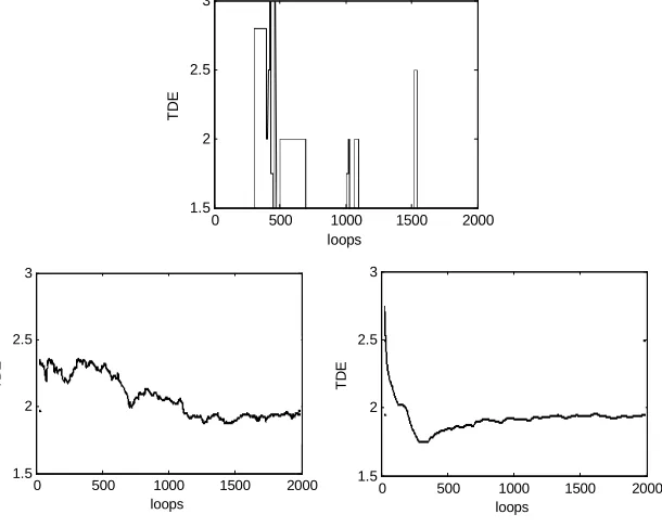
Experiment 2 Time delay estimation invariable SNR
When SNR reduced from 0dB to -10dB, compare the delay estimation. The first 1000 data with SNR=0dB, the last
1000 data with SNR=-10dB.The optimal solution of the gain factor in FOC-ETDGE method is *
=
0
.
09
g
, whenSNR=-10dB the optimal solution is *
=
0
.
5
g
. In FOC-ETDE method, g is fixed to 1. In Figure 3 we compare their performance in variable SNR. Obviously, FOC-LMSTDE algorithm gets incorrect TDE, the effect of FOC—ETDEEis not good, which is because that any change in the filter parameters is considered to be a change in the time delay, so TDE can not be tracked in time. In contrast, the effect of the improved algorithm is the best, even in the case of a large change to SNR, it can also be converged to the estimated value 2.
(a) FOC-LMSTDE (b) FOC-ETDE (c) The proposed algorithm Figure 3: TDE in variable SNR
CONCLUSION
In this paper an improved adaptive time delay estimation algorithm based on four order cumulants is proposed. The single adaptive filter is separated into two adaptive subunits connected in cascade, which making the adaptive process of time delay and signal to noise ratio to be separated, avoiding the poor performance of delay estimation in variable SNR. Simulation results demonstrate the effectiveness of the proposed algorithm.
Acknowledgments
This work was supported by projects of Sichuan Provincial Department of Education(13ZB0138) and projects of Artificial Intelligence Key Laboratory Of Sichuan Province(2013RYY02).
0 500 1000 1500 2000
1.5 2 2.5 3
loops
T
D
E
0 500 1000 1500 2000
1.5 2 2.5 3
loops
T
D
E
0 500 1000 1500 2000
1.5 2 2.5 3
loops
T
D
E
0 500 1000 1500 2000
1.5 2 2.5 3
loops
T
D
E
0 500 1000 1500 2000
1.5 2 2.5 3
loops
T
D
[image:5.595.78.542.475.643.2]REFERENCES
[1] LIU Ying, WANG Shu-xun, WANG Ben-ping, Journal of System Simulation, 2002, 14(6), 700-703
[2]LI Cong-ying, WANG Jian-ying, YIN Zhong-ke, ZHANG Jiang-li, Journal of the China railway society, 2006, 28(6), 55-58
[3] ZHANG Duan-jin ZHANG Zhong-hua GUO Jian-jun ZHANG De-jing, Journal Of Zhengzhou
University(Engineeringscience), 2010,31(1), 103-106
[4]H.C.So and P. C. Ching. A novel constrained time delay estimator . Proc. Of ICSP’93. Beijing China. 1993, 188-192
[5]XIONG Qiu-ben, WANG Jiang, YANG Jing-shu, Electronic Warfare Technology, 2011, 26(3), 10-15
[6]Faramarz Fekri, Mina Sartiipi and Resssell M. Mersereau. IEEE Transactions on Signal Processing. May 2005, 53(5)