Vol. 2, No. 2, pp. 113-126, April (2019)
Double-Objective Optimization Based on Movement
Dynamics of Charged Particles
Vahab Nekoukar
Department of Electrical Engineering, Shahid Rajaee Teacher Training University, Tehran, Iran
Double-objective optimization is a wide class of multi-objective optimization problems in different scientific and industrial applications. This paper proposes a method for the problem of constrained double-objective optimization that is called gravitational charged particles optimization (GChPO). The presented algorithm is based on the movement dynamics of charged particles in the electric field. The mass and electric charge of particles vary according to the value of the first and second objective function, respectively. Usually, in multi-objective optimization algorithms, the dominant and non-dominant solutions should be determined in every iteration, which increases the computation cost of the algorithm. In the proposed method, there is no need of determining the dominant and non-dominant solutions in every iteration that decreases the computation time of the algorithm, significantly. Performance of GChPO is evaluated by seven double-objective and four single-objective benchmark problems. The obtained results are compared with the recent multi-objective and well-known single-objective optimization algorithms that indicate not only the presented algorithm can find the Pareto solutions in the double-objective functions but also it performs better than other algorithms, generally.
Article Info
Keywords:
Double-objective optimization with constraints
electric force; gravitational force; meta-heuristic algorithm Article History:
Received 2018-09-30
Accepted 2018-12-16
I.INTRODUCTION
Nowadays, optimization is applied in many fields of science especially engineering [1-5]. To solve an optimization problem, an engineer should model the system at first, based on his/her engineering view and obtain proper objective function(s) and constraints. Then he/she can solve the problem, mathematically. Scientists have proposed various optimization methods in the literature but there is no guarantee that the problem has a continuous mathematical objective function(s) of the control variables that makes gradient-based optimization techniques useless. To deal with these problems, direct search methods have been introduced to many kinds of research [6]. Direct search only needs an objective function(s) and constraints. However, it may be slow because objective function is evaluated many times for finding the optima, therefore, it is time-consuming.
Many optimization algorithms have been proposed based on the natural phenomena such as biological, physical and
chemical processes and events that are called meta-heuristic optimization method consists of search sub-algorithms, which search the feasible domain. Inspired by behavior in various biological populations, some artificial evolutionary algorithms (EA) have been proposed [7-11]. Genetic algorithm (GA) is one of the famous EA that is based on natural selection, genetic recombination, and mutation [7]. Other conventional EA are ant colony optimization (ACO) [12], particle swarm optimization (PSO) [9], artificial bee colony (ABC) algorithm [10], cuckoo search [13, 14] and grey wolf optimizer [15].
Recently, researchers have introduced optimization methods based on physical laws. Rashedi et al [16] proposed a gravitational search algorithm (GSA) based on the law of gravity and mass interactions i.e. Newtonian gravity. In this algorithm, a population is a set of particles with mass. Individuals interact with each other based on the Newtonian gravity and Newton’s second law of motion. Mass of the particles is proportional to their performance. Performance is determined by the objective function value of the particles by
Corresponding Author: [email protected]
Tel: +98-21-22970006, Fax: +98-21-22970006
Department of Electrical Engineering, Shahid Rajaee Teacher Training University, Iran.
A
B
S
T
R
A
C
means of particle position. Particles with heavier masses attract the other particles and move slowly.
In other work, Kaveh et al [17] introduced a new meta-heuristic algorithm called magnetic charged system search (MCSS) which is an improved version of the charged system search (CSS) algorithm. MCSS is based on the magnetic and electric forces. Charged particles make a population and their Lorentz forces acting on the other particles are varied by related particle performance.
Many optimization problems in engineering are usually multiple objectives that their Pareto-optimal solutions are a set of optima instead of a single optimal solution and usually, there is no any best solution. Over the past decades, many multi-objective algorithms have been presented [18-23]. The inheritance non-dominated sorting genetic algorithm (NSGA) is one of the most famous algorithms [18]. In constraint satisfaction, multi-objective problems on infinite search domains, finding the Pareto-optimal solutions is often difficult. In the conventional and some new methods of multi-objective optimizations [18-20], the dominant and non-dominant particles or chromosomes should be found in every iteration. It makes the algorithm time-consuming especially by increasing the population or running iterations of the algorithm.
In this paper, we present a novel meta-heuristic optimization algorithm based on a motion of charged particles with mass in the electric field. The equation of particles’ motion is written based on Newton’s second law of motion. The proposed optimization algorithm is called gravitational charged particles optimization (GChPO) that is presented for constrained double-objective optimization problems. The GChPO algorithm tries to find the Pareto solutions on the Pareto front with no need of determining the dominant and non-dominant particles in every iteration that makes the proposed algorithm faster than the other algorithms in this category.
The experiment results of double-objective optimization obtained by GChPO algorithm is compared with the elitist non-dominated sorting genetic algorithm with inheritance (i-NSGA-II) [19], multi-objective simplified swarm optimization with weighting scheme for gene selection (MOSSO) [20], multi-objective bacteria foraging optimization algorithm (MOBFOA) [21], modified PBI (MPBI) [22] and multi-objective improved teaching– learning-based optimization algorithm (MO-ITLBO) [23]. In addition, GChPO algorithm is compared with GA, PSO and ABC algorithms in the optimization problem of four single-objective functions.
The rest of the paper is organized as follows. The second section contains the phenomena and mathematical model of the electric fields. Section three deals with the design of the proposed simulated electric field optimization method based on the facts described in section two. In the fourth section,
the experiment results of the proposed method and related discussions are given. Paper contains are concluded in section five.
II.THEORETICAL BASICS
In this section, basic concepts of electric field, gravity and Newton’s second law are presented. These concepts are the foundation of the proposed optimization algorithm.
A.Electric field
Every point charge produces an electric field around it. Michael Faraday defined the electric field at a given point as the electric force (Coulomb) per unit charge. The electric
field (E
r
), can be written as
e F E
q =
r r
(1)
where
F
er
is the exerted force on a particle with charge q
[24]. The electric field of a point charge is also calculated based on the Coulomb's law, which describes force applied on first static point charge (Q1) by second static point charge
(Q2) as 1 2
12 3 12
e e
q q
F K r
r
= ⋅
r r
(2)
that Ke = 8.99×10⁹ N.m
2
.C−2 is Coulomb's constant, q1 and q2
are signed magnitudes of the point charges and rr12 =rr1−rr2
is the vectorial distance between the charges. The force of interaction between the charges is attractive if the charges have opposite signs and vice versa [24].
B.Gravity
Each mass particle attracts every other mass particles around itself. This natural phenomenon is called gravity. The most familiar aspect of the gravity is Newton’s apple. Based on Newton's law of gravity, the attraction force between two bodies is directly proportional to the product of their masses and inversely proportional to the square of the distance between them [25]. The gravitational force between two
particles (
F
gr
) can be written
1 2
21 3 21
g
m m
F G r
r
= ⋅
r r
(3)
where G = 6.67×10⁻¹² m3.kg−1.s−2 is gravitational constant, m1
and m2 are mass of the particles and r21=r2−r1
r r r
is the
vectorial distance between them. It is clear that mass gaining of the particles increases the gravitational force.
C.Newton’s second law
formulated as
net F =ma
r r
(4)
where Fnet r
is the net force acting on the particle, ar is particle acceleration and m is particle mass. Equ. (4) shows that the direction of the acceleration vector is the same as net force vector [25]. Velocity, v(t), and position, x(t), of the particles are calculated as
0 0
( ) ( )d
t
v t =v +
∫
aτ
τ
(5)0 0
( ) ( )d
t
x t =x +
∫
vτ
τ
(6)where x0 and v0 are the initial position and velocity of the
particle, respectively.
III.
GRAVITATIONAL CHARGED PARTICLESOPTIMIZATION (GCHPO)METHOD
In this section, the GChPO method is introduced based on the theoretical background explained in section 2. In this method, optimizing variables are considered as charged particles with mass, which can move in space without any friction. Acceleration of the particles is dependent on the net force acting on the particles. The net force is a vector sum of the electric and gravitational forces exerted on the particles. The push or pull exerted force causes acceleration or deceleration of the particles in the space. Movement of every particle has a specific dynamics that is indicated by Newton’s second law. Heavier particles produce bigger attractive forces and particles with higher charge generate stronger attractive or repulsive forces. Then, mass and charge of particles are determined by their performance. We just consider the electric force as attraction and polarity of the particles is ignored. Better particles pull other particles around themselves; therefore, particles gather around the better ones, by lapse of time and produce different solution groups.
The GChPO algorithm is proposed for double-objective problems. The charge of the particles is varied based on the first objective function and mass of particles is determined depending on the second objective function. Therefore, mass and charge of the particles are independent. One advantage of the presented algorithm is that a set of solutions is obtained because, in the end, each particle group is a solution in the admissible search space.
For preventing the early convergence and sticking in local optima, two strategies are suggested. First, we consider a friction-like force that acts as a kinetic friction and resists motion of particles in space. This resistive force obtains momentum-like property. The second strategy is a random electric field that is generated in the search space and it exerts a repulsive electric force on the particles. It makes particles’ movement relative to their mass. The direction of the repulsive electric force is also random. Emersion chance of
the random electric field is decreased by lapse of time. To deal with conditional problems with known constraints, we consider repulsive electric fields in the infeasible search space that push the infeasible particles to the feasible space. The direction of the electric field is randomly determined.
At the beginning of the proposed algorithm, N particles are located in the search space, randomly. Each particle is shown by p. Position, velocity and acceleration vectors of the ith particle at time t are respectively defined as
1 2 1 2 1 2 ( ) [ ( ), ( ), , ( )] ( ) [ ( ), ( ), , ( )] ( ) [ ( ), ( ), , ( )] n
i i i i
n
i i i i
n
i i i i
x t x t x t x t v t v t v t v t a t a t a t a t
= = = r K r K r K
that n is dimension of the search space, ( ), ( ) and ( )
j j j
i i i
x t v t a t is ith particle position, velocity, and acceleration in jth dimension at time t, respectively. For every particle, we can write
( ) ( ) ( ) ( )
net elec grav fric
i i i i
F t =F t +F t +F t
r r r r
(7) 3 1 ( ) ( ) ( ) ( ) ( ) ( ) ( ) N i j elec
i i rand ij
j ij j i
q t q t
F t q t E t r t
r t = ≠
= +
∑
r r r
r (8) 3 1 ( ) ( ) ( ) ( ) ( ) N i j grav i ji j ji j i
m t m t
F t r t
r t = ≠ =
∑
r r r (9) ( ) ( ) ( ) ( ) fric ii k i
i v t
F t gm t
v t µ = − r r r (10)
where Finet r
is a total force acting on the ith particle, ( ) , ( ) and ( )
elec grav fric
i i i
F t F t F t
r r r
are an electric force,
gravitational force and friction force applied on the ith particle, respectively. Erand( )t
r
is a random electric field that
exerts a random force on all the particles at time t. µk is
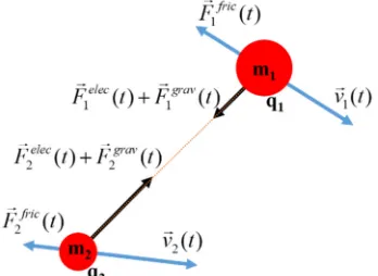
coefficient of kinetic friction between 0 to 1 and g is the acceleration of gravity (9.8 m/s2). Mentioned force vectors for two particles are shown in Fig. 1.
Acceleration, velocity, and position of ith particle are calculated as ( ) ( ) ( ) net i i i F t a t m t = r r (11)
( )
( ) ( )
( 1)
i v i i
v t
r
=
r t a t
r
+
v t
r
−
(12)( )
( ) ( )
(
1)
i x i i
x t
r
=
r t v t
r
+
x t
r
−
(13)( ) and ( )
i i
q t
m t
are dependent on the value of the first andsecond objective functions, respectively.
r t
v( ) and ( )
r t
x
Fig. 1. Diagram of electric and gravitational forces for two assumed particles
If we assume that the first objective function is
J x t
1( ( ))
and the second objective function is
J x t
2( ( )),
we candetermine
q t
i( ) and ( )
m t
i as1
2( 1 (t 1))
( )
( 1)
i i
N N
m t
N N
+ − −
=
+ (14)
2
2( 1 (t 1))
( )
( 1)
i i
N N
q t
N N
+ − −
=
+ (15)
1 2
( ) and ( )
i i
N t N t are rank of ith particle among the whole N
particles at time t based on evaluation and sorting of the first (J1) and second (J2) objective functions, respectively. For
example, N1i =1 for the best particle at time t and Ni1=N
for the worst particle, based on J1 evaluation.
The probability of appearing a random electric field (
E
randr
in Equ. (8)) that exerts a random electric force on all the particles, according to the prevention of the early convergence, is p(t). We call p(t) appearing probability function that is defined as
( ) t p t eτ −
= (16)
where τ is a positive constant. p(t) converges to zero, exponentially. Magnitude and direction of Erand
r
is randomly
determined. The maximum value of the field magnitude
(maximum of
E
randr
) is Emax.
The parameter µk is the friction coefficient. The small
value of µk reduces the frictional force so its effect is lost.
The large amount of µk makes the particles’ movement
difficult. The value of µk should be selected by comparing the
amount of the frictional force with both electric and gravitational forces in Equ. (7). The parameter Emax is the
maximum value of Erand. The low value of this parameter
reduces the effect of the random electric force in (8) and the high value causes divergence of the proposed algorithm. The range of the second term in Equ. (8) determines the proper value of Emax. The parameter τ controls the appearing
probability of the random electric field Erand. Increasing the
parameter τ increases the appearing probability of the Erand.
The GChPO algorithm is described in the following steps:
(1)Selection of algorithm parameters (N, µk, τ and Emax)
(2)Randomly initialize the position of particles (3)Set initial values of velocity and acceleration of the
particles equal to zero (4)FOR (i = 1:N)
(a)Fitness evaluation of particles (J x1i( (0))i and
2( (0)) i
i J x )
(b)Sort particles and determine Ni1(0) and Ni2(0)
(5)t = 1
(6)WHILE (t <= maximum number of iterations) (a)Calculation of Equ. (14)
(b)Generate a random number in [0, 1] (c)If p(t) > generated random number in step b (d)Generate a random electric field
(e)FOR (i = 1:N)
(i)Calculation of Equs. (12) and (13) (ii)Calculation of Equ. (5)
(iii)updating ai(t) and vi(t)
(iv)calculation of xi(t)
(v)Fitness evaluation of particles ( 1( ( )) i
i J x t
and 2i( ( ))
i J x t )
(f)Sort particles and determine N ti1( ) and N ti2( )
(g)If stop criteria are reached (i)ENDWHILE
(h)t = t +1 (7)Present the best particles
(8)End
The flowchart of the proposed method is presented in Fig. 2. The stop criteria can be a time limitation, an acceptable minimum value of objective functions and other conventional stop criteria.
IV.
EXPERIMENT STUDIESTABLEI
TUNED PARAMETERS OF GCHPOALGORITHM
50
N
=
Emax=1µ
k =0.1τ =
100
Fig. 2. Flowchart of the proposed optimization method (GChPO)
A.Optimization of Zitzler–Deb–Thiele's Function 1
The formula of Zitzler–Deb–Thiele's function 1 (ZDT1) is written as
1 1
30
2
1 2
( )
9 ( ) 1
29
( ) ( ) 1
( ) i i f x x
g x x
x f x g x
g x =
=
= +
= −
∑
0≤xi≤1 (17)
where x=[ ,x x1 2,..., x ]30 T is a searchable variable vector, f1
and f2 are objective functions. The experiment results of
optimization algorithms are shown in Fig. 3 for iterations 100, 200, 300 and 400 with the true Pareto front of ZDT1 function.
The results of GChPO algorithm demonstrate the good behavior of particles during the optimization. Particles of GChPO converged on near of the true Pareto front before iteration 100 as same as MOSSO. These two algorithms are the fastest. Convergence speed of GChPO was much faster than MO-ITLBO and I-NSGA-II. All particles of GChPO population are non-dominant in iteration 400. Fig. 3 (d) shows that GChPO and MOSSO particles are distributed on the whole of the true Pareto front, properly but surprisingly, I-NSGA-II did not cover the entire true Pareto front.
B.Optimization of Zitzler–Deb–Thiele's function 2
Zitzler–Deb–Thiele's function 2 (ZDT2) is described as
1 1
30
2
2 1 2
( ) 9 ( ) 1
29
( ) ( ) 1 ( ) i i
f x x
g x x
x f x g x
g x
= =
= +
= −
∑
0≤xi≤1 (18)
where x=[ ,x x1 2,..., x ]30 T is a searchable variable vector, f1
and f2 are objective functions. Optimization results are given
in Fig. 4 for iterations 100 and 400. It is clear that MO-ITLBO did not find the Pareto solutions. MOBFOA and MPBI need more iteration and GChPO, I-NSGA-II and MOSSO had acceptable results at the end but Fig. 4 (a) shows interested convergence speed of the GChPO. Obtained solution by I-NSGA-II is not proper in iteration 100.
C.Optimization of Zitzler–Deb–Thiele's function 3
Zitzler–Deb–Thiele's function 3 (ZDT3) is written as
1 1
3 0
2
1 2
1
1
( ) 9 ( ) 1
2 9 ( ) ( ) 1
( ) s in (1 0 )
( )
i i f x x
g x x
x f x g x
g x
x
x
g x π
=
=
= +
= −
−
∑
(a)
(b)
(c)
(d)
Fig. 3. Pareto solution obtained by optimization of ZDT1 for (a) iteration = 100, (b) iteration = 200, (c) iteration = 300 and (d) iteration = 400.
where T
1 2 30
[ , ,..., x ]
x= x x is a searchable variable vector, f1
and f2 are objective functions. The experiment results of
ZDT3 optimization are shown in Fig. 5. Solving this problem is harder that ZDT1 and ZDT2. The results confirm the high convergence speed of GChPO, in contrast to the other algorithms, to the true Pareto front. GChPO particles distributed overall the true Pareto front very well but finding all points on the true Pareto front cannot be accomplished by I-NSGA-II, MO-ITLBO, MOBFOA, and MPBI.
D.Optimization of Zitzler–Deb–Thiele's function 6
Zitzler–Deb–Thiele's function 6 (ZDT6) is calculated as
6
1 1 1
0.25 10
2
2 1 2
( ) 1 exp( 4 ) sin (6 )
( ) 1 9 9
( ) ( ) ( ) 1
( ) i i
f x x x
x g x
f x f x g x
g x
π
=
= − −
= +
= −
∑
0≤xi≤1 (20)
where x=[ ,x x1 2,..., x ]10T is a searchable variable vector, f1
and f2 are objective functions. The experiment results of
ZDT6 optimization are shown in Fig. 5 for iteration 100 and 400. I-NSGA-II have a better distribution and it outperformed GChPO but MOSSO and MOBFOA were as same as GChPO in iteration 400. MPBI and MO-ITLBO appeared weaker than the others did.
(a)
(b)
(a)
(b)
(c)
(d)
Fig. 5. Pareto solution obtained by optimization of ZDT3 for (a) iteration = 100, (b) iteration = 200, (c) iteration = 400 and (d) iteration = 500.
(a)
(b)
Fig. 6. Pareto solution obtained by optimization of ZDT6 for (a) iteration = 100 and (b) iteration = 400. There is no point under the figure legend.
E.Optimization of Binh and Korn function
The Binh and Korn (BK) function is written as
2 2
1 1 2
2 2
2 1 2
( ) 4 4
( ) (x 5) (x 5)
f x x x
f x
= +
= − + −
1
2
0 5
0 3
x
x
≤ ≤
≤ ≤
(21)
2 2
1 2
2 2
1 2
s. t .
(x 5) x 25
(x 8) (x 3) 7.7
− + ≤
− + + ≥
where x=[ ,x x1 2]T is a searchable variable vector, f1 and f2
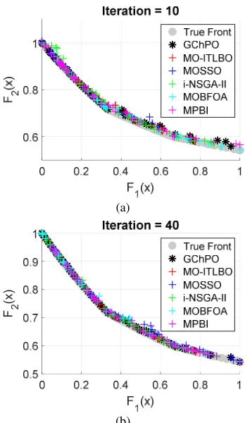
are objective functions. The experiment results are shown in Fig. 7 indicate that all algorithms overcame the challenge. The GChPO algorithms found the true Pareto front before iteration 10. Fig. 7 (b) explains that the GChPO particles distributed on the Pareto front, almost uniformly. Therefore, constrained optimization problems are not a limitation for GChPO algorithm.
0 0.2 0.4 0.6 0.8 1
F
1(x)
-1 0 1 2
3 Iteration = 100
True Front GChPO MO-ITLBO MOSSO i-NSGA-II MOBFOA MPBI
0 0.2 0.4 0.6 0.8 1
F1(x)
-1 0 1 2
3 Iteration = 200
0 0.2 0.4 0.6 0.8 1
F
1(x)
-1 0 1 2
F 2
(x
)
Iteration = 500
F.Optimization of Osyczka and Kundu function
Osyczka and Kundu (OK) function and its constraints are explained as
2 2
1 1 2
2 2
3 4
2 5 6
2 2
1
( ) 25( 2) ( 2)
( 1) ( 4)
( 1)
( ) i
i
f x x x
x x
x
f x x
=
= − − − −
− − − −
− −
=
∑
1 2 6
3 5
4
0 , , 10
1 , 5
0 6
x x x x x
x
≤ ≤
≤ ≤
≤ ≤
(22)
1 2
1 2
2 1
1 2
2
4 3
2
5 6
s.t.
2 6 2
3 2
x (x 3) 4
(x 3) x 4
x x x x x x x x
+ ≥
+ ≤
− ≥
− ≥
+ − ≤
− + ≥
where x=[ ,x x1 2,..., x ]6 Ta is a searchable variable vector, f1
and f2 are objective functions. This problem is the most
difficult among all benchmark functions represented in this paper. The experiment given in Fig. 8 demonstrates that there is no winner. GChPO and I-NSGA-II outperformed the other algorithms. However, MO-ITLBO is out of the league. I-NSGA-II and GChPO were able to find the most points of the true Pareto front, respectively.
(a)
(b)
Fig. 7. Pareto solution obtained by optimization of BK for (a) iteration = 10 and (b) iteration = 40.
(a)
(b)
(c)
(d)
Fig. 8. Pareto solution obtained by optimization of OK for (a) iteration = 200, (b) iteration = 1000, (c) iteration = 1500, (d) iteration = 2000.
F 2
(x
)
F 2
(x
G.Optimization of CTP1 function
CTP1 function is calculated as
1 1
1
2 2
2
( )
( ) (1 ) exp( ) 1
f x x
x
f x x
x =
= + −
+
0≤xi≤1
(23)
2
1
2
1
s.t.
( )
1 0.858exp( 0.541 ( ))
( )
1 0.728exp( 0.295 ( ))
f x f x f x
f x
≥
−
≥
−
where x=[ ,x x1 2]T is a searchable variable vector, f1 and f2
are objective functions. The optimization results of CTP1 are demonstrated in Fig. 9. All algorithms came up with a solution to the problem. GChPO, MOSSO, MOBFOA, and MPBI were able to find the lower points on the true Pareto front (0.9≤ f x1( )≤1).
(a)
(b)
Fig. 9. Pareto solution obtained by optimization of CTP1 for (a) iteration = 10 and (b) iteration = 40.
H.Performance metrics
In this section, using the three criteria (generational distance, spacing and hyper-volume ratio), the performance of the proposed algorithm is compared with the rest of the algorithms. Generational distance (GD) explains the average
distance between obtained Pareto front by algorithms and real Pareto front of the problem. GD is a conventional performance metric for performance evaluation of multi-objective optimization algorithms [26]. If P and A are a set of real and obtained Pareto front, respectively then the generational distance between P and A is defined as
1
( , ) ( , )
N
i i i
d x v GD P A
N = =
∑
(24)where N is the number of obtained solutions in A, xi is i
th
member of A, vi is a member of P that is nearest neighbor of xi and d is the Euclidian distance between xi and vi. The lower
value of GD means better convergence of the obtained optimal solutions to the real Pareto front.
Table II shows average GD obtained by 20 runs of optimization for every benchmark function. The optimization results of ZDT1, BK, and CTP1 benchmark functions explain that GD of the proposed method is significantly less than other algorithms. It means that GChPO was more successful in finding the real Pareto front after limited iterations of running. Average GDs of GChPO and MOSSO are very close for ZDT2 and ZDT3 functions. These results are the best with the significant difference in contrast to the entire algorithms for the mentioned benchmark functions. All experimented algorithms except MO-ITLBO had acceptable performance in ZDT6 optimization. The OK benchmark function is the most challengeable problem. Based on the obtained GD and Fig. 8, the performance of i-NSGA-II is the best but performance of GChPO is also acceptable. GChPO could not find solutions on the top of real Pareto front where i-NSGA-II could search. The other optimization algorithms failed in this benchmark problem.
Table III shows the adjusted p-values for the Friedman test based on the Holm test with respect to the results given in Table II [27]. To calculate p-values, GChPO was the control method, which has the first Friedman rank equals 1.29.
The spacing represents the distribution of Pareto solution in objective space. It is also a criterion to evaluate the convergence of the obtained results [19]. The spacing is defined as
2
1
( , ) ( , )
N
i i i
d d x v S P A
N =
−
=
∑
(24)where d is the mean value of Euclidian distances. S = 0 explains that the distribution of the solution is uniform.
F 2
(x
TABLEII
AVERAGE GDPERFORMANCE METRIC OF DOUBLE-OBJECTIVE OPTIMIZATIONS IN 20RUNS
Benchmark Function Iteration GChPO i-NSGA-II MOSSO MOBFOA MPBI MO-ITLBO
ZDT1 400 0.0163 0.0751 0.0230 0.1547 0.0954 0.0830
ZDT2 200 0.0187 0.8140 0.0202 0.2858 0.1709 1.1461
ZDT3 500 0.0270 0.0982 0.0271 0.1049 0.1353 0.3597
ZDT6 400 0.0171 0.0125 0.0178 0.0354 0.0179 4.5564
BK 40 1.1653 1.5020 1.8179 2.0492 1.9701 11.9093
OK 2000 8.3123 4.5386 28.6350 32.0433 23.2527 128.2068
CTP1 40 0.0104 0.0214 0.0149 0.0263 0.0163 0.0478
TABLEIII
ADJUSTED P-VALUES FOR THE FRIEDMAN TEST BASED ON THE
HOLM TEST (GCHPOWAS THE CONTROL METHOD)
Algorithm Average Friedman Rank p-value MOSSO 2.57 0.011955 i-NSGA-II 2.71 0.0056768
MPBI 3.86 6.081e-06 MOBFOA 4.86 1.1319e-08 MO-ITLBO 5.71 6.8695e-11
The average spacing obtained by 20 runs of optimization for every benchmark function is given in Table IV. The results show that GChPO and i-NSGA-II have the most uniform distribution of the solutions on the real Pareto front. As the previous results showed, MO-ITLBO had not an acceptable performance for both BK and OK benchmark functions.
Hyper-volume ratio (HVR) is the ratio of hyper-volumes made by the obtained and real Pareto fronts according to a reference point in the dominated region [28]. The best value of HVR is one that means the obtained solutions and the Pareto solutions are very close to each other with a uniform distribution. Table V demonstrated the average HVR obtained by 20 runs of optimization for every benchmark
function. Overly, MPBI has the best HVR values. The mean of the HVR values is 0.57 for both GChPO and MOBFOA and MO-ITLBO is the worst.
I.Optimization of single-objective benchmarks
The GChPO algorithm is presented to solve the double-objective problems or any multi-objective problem that can be transformed into a double-objective problem. However, it is shown in this section that the proposed algorithm can be also applied to optimize single-objective problems, such as well-known GA, PSO and ABC algorithms. To prove this, four benchmark problems have been used. The specifications of the benchmark functions are given in Table VI.
The mean and standard deviation of the best solution for 20 experiment runs are shown in Table VII. The results obtained by GChPO are compared with GA, PSO and ABC algorithms. In all experiments and for all algorithms, the number of iterations is 100 times and the number of the population is 50. The stop criterions of the algorithms are the 100-time execution or cost function tolerance less that 1e-6.
TABLEIV
AVERAGE SPACING METRIC OF DOUBLE-OBJECTIVE OPTIMIZATIONS IN 20RUNS
Benchmark Function Iteration GChPO i-NSGA-II MOSSO MOBFOA MPBI MO-ITLBO
ZDT1 400 0.00 0.01 0.03 0.00 0.00 0.00
ZDT2 200 0.00 0.00 0.00 0.08 0.01 0.32
ZDT3 500 0.00 0.03 0.00 0.01 0.02 0.20
ZDT6 400 0.00 0.00 0.00 0.00 0.00 2.32
BK 40 2.05 4.06 5.73 9.99 7.55 313.52
OK 2000 167.24 32.14 1322.80 1568.50 959.94 1352.10
CTP1 40 0.00 0.00 0.00 0.00 0.00 0.01
TABLEV
AVERAGE HVR PERFORMANCE METRIC OF DOUBLE-OBJECTIVE OPTIMIZATIONS IN 20 RUNS
Benchmark Function Iteration GChPO i-NSGA-II MOSSO MOBFOA MPBI MO-ITLBO
ZDT1 400 0.65 0.57 0.64 0.68 0.69 0.53
ZDT2 200 0.33 0.31 0.30 0.31 0.48 0.07
ZDT3 500 0.72 0.70 0.76 0.74 0.76 0.048
ZDT6 400 0.50 0.30 0.36 0.55 0.59 0.00
BK 40 0.73 0.74 0.73 0.75 0.69 0.54
OK 2000 0.79 0.83 0.70 0.65 0.72 0.08
CTP1 40 0.28 0.26 0.28 0.28 0.27 0.24
TABLEVI
SPECIFICATIONS OF FOUR SINGLE-OBJECTIVE BENCHMARK PROBLEMS
Benchmark
Function Formula Input Domain
Global Minimum
Shubert
(
)
(
cos((
1
)
)
)(
cos((
1
)
)
)
5 1 2 5 1 1
∑
∑
= =+
+
+
+
=
i ii
x
i
i
i
x
i
i
x
f
x
i∈
[-5.12, 5.12] -186.7Rastrigin
∑
=
−
+
=
2 1 2)]
2
cos(
10
[
20
)
(
i i ix
x
x
f
π
x
i∈
[-5.12, 5.12] 0Schwefel
5
1
( )
418.9829*5
( sin(
i i)
i
f x
x
x
=
=
−
∑
x
i∈
[-500, 500] 0Ackley
cos(
2
)
)
20
exp(
1
)
2
1
exp(
)
2
1
2
.
0
exp(
20
)
(
2 1 2 1 2+
+
−
−
−
=
∑
∑
= = i i i ix
x
x
f
π
x
i∈
[-32.8, 32.8] 0For three benchmark functions Shubert, Rastrigin and Ackley, GChPO, PSO and ABC demonstrate the good performance in contrast with GA. GA is a slower algorithm then it needs more generation to achieve a better solution. Schwefel benchmark problem is much more difficult than the others are. None of the algorithms has an acceptable performance for this problem. However, GA and GChPO have the best results.
J.Computation time
In this section, the computation time of GChPO is compared with i-NSGA-II, MOSSO, MOBFOA, MPBI and MO-ITLBO for seven double-objective benchmark problems and with GA, PSO, and ABC for four single-objective benchmark problems. Every optimization algorithm was done 20 times for every benchmark functions then average computation time is given in Table VIII and IX for double-objective and single-objective benchmark problems, respectively. Table VIII shows lower computation cost of GChPO in comparison of i-NSGA-II, MOBFOA, MPBI, and MO-ITLBO but MOSSO is generally faster than GChPO nevertheless GChPO is more successful to find the Pareto solutions.
Table IX presents the average computation time for four single-objective benchmarks. GChPO is not the fastest algorithm. However, its computation cost is lower than the ABC algorithm. The computation time of PSO and GChPO is almost equal. The average of total computation time of GA is 3.5 ms more that GChPO that is negligible. It is notable that the purpose of proposing GChPO is to solve the double-objective optimization function. Table V shows the superiority of computation cost for the proposed method. The experiment of single- objective optimization is just because we show that GChPO can solve these type of problems, too.
V.CONCLUSIONS
A new meta-heuristic algorithm called GChPO was proposed for constrained double-objective optimization. The presented algorithm is based on the movement of the charged particles in the electric field based on Newton’s second law of motion. Three different forces effect on the particle movement: gravitational, electric force and friction forces. The superposed force accelerates the particles. Performance of GChPO was compared with different optimization algorithms on a set of seven double-objective and four single-objective benchmark problems. The experiment results explain that the proposed algorithm generally outperformed the rest of the optimization algorithm.
TABLEVII
IMPLEMENTATION RESULTS OF FOUR SINGLE-OBJECTIVE
BENCHMARK PROBLEMS
Benchmark Function Average of
best minimum Algorithm
Shubert
-186.73 ± 0.00 GChPO -186.73 ± 0.00 PSO -181.36 ± 24.00 GA
-186.73 ± 0.01 ABC
Rastrigin
0.00 ± 0.01 GChPO 0.00 ± 0.02 PSO 0.15 ± 0.36 GA 0.00 ± 0.00 ABC
Schwefel
172 ± 86.12 GChPO 254.92 ± 150.28 PSO 165.55 ± 123.26 GA
371.50 ± 93.28 ABC
Ackley
TABLEVIII
AVERAGE COMPUTATION TIME FOR SEVEN DOUBLE-OBJECTIVE BENCHMARKS IN 20RUNS
Benchmark Function GChPO (Sec)
i-NSGA-II (Sec)
MOSSO (Sec)
MOBFOA (Sec)
MPBI (Sec)
MO-ITLBO (Sec)
ZDT1 38.49 140.52 16.01 85.28 182.90 138.03
ZDT2 13.39 53.15 11.24 26.59 100.61 72.12
ZDT3 49.11 163.96 30.27 103.85 210.00 180.03
ZDT6 24.11 99.49 24.65 70.25 182.92 144.18
BK 4.74 9.77 3.26 9.25 10.15 11.00
OK 138.72 736.96 88.99 392.26 443.01 677.41
CTP1 3.21 10.58 3.36 9.86 10.38 12.11
TABLEIX
AVERAGE COMPUTATION TIME FOR FOUR SINGLE-OBJECTIVE BENCHMARKS IN 20RUNS
Benchmark Function GChPO (Sec)
GA (Sec)
PSO (Sec)
ABC (Sec)
Shubert 0.1978 0.1483 0.2083 0.2081
Rastrigin 0.1312 0.1500 0.1251 0.2115
Schwefel 0.2228 0.2647 0.2084 0.3835
Ackley 0.1573 0.1602 0.1532 0.2279
Average 0.1773 0.1808 0.1738 0.2578
One of the main challenges in the implementation of multi-objective optimization algorithms is that these algorithms are time-consuming. One of the conventional solutions to this problem is to use parallel processing. In the future works, we will try to propose a solution to the parallel implementation of the proposed algorithm on different processors. In addition, for the particles, we will consider the magnetic property. Therefore, around the particle, a magnetic field can also be created which can be applied a magnetic force to the particles. Same as mass and electric charge of the particles, their magnetic charge can be determined based on a different cost function, so such an algorithm can be applied to solve the triple-objective optimization problems.
A
PPENDIXThe parameter setting of algorithms is
i-NSGA-II: pc = 0.85, pm = 0.15, w1/w3 = 10 7
/5×108 and
w2/w4 = 10 7
/5×108;
MOBFOA:Ns = 6, Nc = 35, M = 30, Ned = 6, Ped = 0.25 and s(i) = 1.8;
MPBI:pc = 0.85, pm = 0.15, ηc = 30, ηm = 20, Mr = 0.7, fr = 0.05 and θ= 7;
MO-ITLBO:number of teacher = 5;
MOSSO:Cg = 0.65, Cp = 0.8 and Cw = 0.95.
REFERENCES
[1] G. Gonzales, E. da SD Estrada, L. Emmendorfer, L. Isoldi, G. Xie, L. Rocha, et al., "A comparison of simulated annealing schedules for constructal design of complex cavities intruded into conductive walls with internal heat generation," Energy,
vol. 93, pp. 372-382, 2015.
[2] V. Khanna, B. Das, D. Bisht, and P. Singh, "A three diode model for industrial solar cells and estimation of solar cell
parameters using PSO algorithm," Renewable Energy, vol. 78, pp. 105-113, 2015.
[3] M. Qiu, Z. Ming, J. Li, K. Gai, and Z. Zong, "Phase-change memory optimization for green cloud with genetic algorithm," IEEE Transactions on Computers, vol. 64, pp. 3528-3540, 2015.
[4] H. Renaudineau, F. Donatantonio, J. Fontchastagner, G. Petrone, G. Spagnuolo, J.-P. Martin, et al., "A PSO-based global MPPT technique for distributed PV power generation," IEEE Transactions on Industrial Electronics,
vol. 62, pp. 1047-1058, 2015.
[5] S. Lyden and M. E. Haque, "A simulated annealing global maximum power point tracking approach for PV modules under partial shading conditions," IEEE Transactions on Power Electronics, vol. 31, pp. 4171-4181, 2016.
[6] T. G. Kolda, R. M. Lewis, and V. Torczon, "Optimization by direct search: New perspectives on some classical and modern methods," SIAM review, vol. 45, pp. 385-482, 2003. [7] J. H. Holland, "Genetic algorithms and adaptation," in
Adaptive Control of Ill-Defined Systems, ed: Springer, 1984, pp. 317-333.
[8] M. Dorigo, M. Birattari, and T. Stutzle, "Ant colony optimization," IEEE computational intelligence magazine,
vol. 1, pp. 28-39, 2006.
[9] J. Kennedy, "Particle swarm optimization," in Encyclopedia of machine learning, ed: Springer, 2011, pp. 760-766. [10] D. Karaboga and B. Basturk, "A powerful and efficient
algorithm for numerical function optimization: artificial bee colony (ABC) algorithm," Journal of global optimization,
vol. 39, pp. 459-471, 2007.
[11] E. Zakeri, S. A. Moezi, Y. Bazargan-Lari, and A. Zare, "Multi-tracker optimization algorithm: a general algorithm for solving engineering optimization problems," Iranian Journal of Science and Technology, Transactions of Mechanical Engineering, vol. 41, pp. 315-341, 2017. [12] M. Dorigo and M. Birattari, "Ant colony optimization," in
Encyclopedia of machine learning, ed: Springer, 2011, pp. 36-39.
[13] X.-S. Yang and S. Deb, "Cuckoo search via Lévy flights," in
[14] S. A. Moezi, E. Zakeri, and A. Zare, "A generally modified cuckoo optimization algorithm for crack detection in cantilever Euler-Bernoulli beams," Precision Engineering,
vol. 52, pp. 227-241, 2018.
[15] S. Mirjalili, S. M. Mirjalili, and A. Lewis, "Grey wolf optimizer," Advances in engineering software, vol. 69, pp. 46-61, 2014.
[16] E. Rashedi, H. Nezamabadi-Pour, and S. Saryazdi, "GSA: a gravitational search algorithm," Information sciences, vol. 179, pp. 2232-2248, 2009.
[17] A. Kaveh, M. A. M. Share, and M. Moslehi, "Magnetic charged system search: a new meta-heuristic algorithm for optimization," Acta Mechanica, vol. 224, pp. 85-107, 2013. [18] K. Deb, A. Pratap, S. Agarwal, and T. Meyarivan, "A fast
and elitist multiobjective genetic algorithm: NSGA-II," IEEE transactions on evolutionary computation, vol. 6, pp. 182-197, 2002.
[19] M. Kumar and C. Guria, "The elitist non-dominated sorting genetic algorithm with inheritance (i-NSGA-II) and its jumping gene adaptations for multi-objective optimization,"
Information Sciences, vol. 382-383, pp. 15-37, 2017/03/01/ 2017.
[20] C.-M. Lai, "Multi-objective simplified swarm optimization with weighting scheme for gene selection," Applied Soft Computing, vol. 65, pp. 58-68, 2018/04/01/ 2018.
[21] M. Kaur and S. Kadam, "A novel multi-objective bacteria foraging optimization algorithm (MOBFOA) for multi-objective scheduling," Applied Soft Computing,
2018/02/15/ 2018.
[22] Q. Zhang, W. Zhu, B. Liao, X. Chen, and L. Cai, "A modified PBI approach for multi-objective optimization with complex Pareto fronts," Swarm and Evolutionary Computation, 2018/02/12/ 2018.
[23] V. K. Patel and V. J. Savsani, "A multi-objective improved teaching–learning based optimization algorithm (MO-ITLBO)," Information Sciences, vol. 357, pp. 182-200, 2016/08/20/ 2016.
[24] D. K. Cheng, Field and Wave Electromagnetics: Pearson New International Edition: Pearson Higher Ed, 2014. [25] R. Resnick, J. Walker, and D. Halliday, Fundamentals of
physics vol. 1: John Wiley, 1988.
[26] H. Ishibuchi, H. Masuda, Y. Tanigaki, and Y. Nojima, "Modified distance calculation in generational distance and inverted generational distance," in International Conference on Evolutionary Multi-Criterion Optimization, 2015, pp. 110-125.
[27] J. Derrac, S. García, D. Molina, and F. Herrera, "A practical tutorial on the use of nonparametric statistical tests as a methodology for comparing evolutionary and swarm intelligence algorithms," Swarm and Evolutionary Computation, vol. 1, pp. 3-18, 2011.
[28] E. Zitzler and L. Thiele, "Multiobjective evolutionary algorithms: a comparative case study and the strength Pareto approach," IEEE transactions on Evolutionary Computation,
vol. 3, pp. 257-271, 1999.
IECO